Marriage and parenthood in relation to obesogenic neighborhood trajectories: The CARDIA Study

Abstract

Marriage and parenthood are associated with weight gain and residential mobility. Little is known about how obesity-relevant environmental contexts differ according to family structure. We estimated trajectories of neighborhood poverty, population density, and density of fast food restaurants, supermarkets, and commercial and public physical activity facilities for adults from a biracial cohort (CARDIA, n=4,174, aged 25–50) over 13 years (1992–93 through 2005–06) using latent growth curve analysis. We estimated associations of marriage, parenthood, and race with the observed neighborhood trajectories. Married participants tended to live in neighborhoods with lower poverty, population density, and availability of all types of food and physical activity amenities. Parenthood was similarly but less consistently related to neighborhood characteristics. Marriage and parenthood were more strongly related to neighborhood trajectories in whites (versus blacks), who, in prior studies, exhibit weaker associations between neighborhood characteristics and health. Greater understanding of how interactive family and neighborhood environments contribute to healthy living is needed.

INTRODUCTION

Marriage and parenthood are strong predictors of weight gain and low diet quality and physical activity (Kahn and Williamson 1990; Sobal, Rauschenbach et al. 1992; Averett, Sikora et al. 2008; Umberson, Liu et al. 2011). Mechanisms underlying these changes are unknown, but may include reduced social pressure to control weight after marriage, additional opportunities to eat through shared eating occasions (Jeffery and Rick 2002; Averett, Sikora et al. 2008), and parenthood-related time constraints as barriers to physical activity (Bellows-Riecken and Rhodes 2008; Brown and Roberts 2011; Ortega, Brown et al. 2011) and healthy eating (Edvardsson, Ivarsson et al. 2011; Bassett-Gunter, Levy-Milne et al. 2013). In particular, families with children face greater time constraints for food preparation and exhibit corresponding increases in away from home eating (Blake, Wethington et al. 2011; Bauer, Hearst et al. 2012).

Environmental factors may contribute to marriage- and parenthood-related weight gain but have not been considered, despite the fact that marriage and parenthood transitions are key drivers of residential mobility (Clark and Withers 2007; Mulder 2007; Cooke 2008; Michielin, Mulder et al. 2008). Neighborhoods may promote healthy body weight by providing physical activity opportunities and healthy food options (Papas, Alberg et al. 2007; Feng, Glass et al. 2010). If young families move into neighborhoods that are less conducive to healthy lifestyles, such environmental changes may contribute to, or exacerbate, obesity-related behavioral shifts observed with marriage and parenthood. Additionally, marriage- and parenthood-related differences in neighborhood characteristics may bias estimates of neighborhood effects on health (Bhat and Guo 2007; Mokhtarian and Cao 2008; Boone-Heinonen, Gordon-Larsen et al. 2011) to the extent that obesity-related neighborhood characteristics are associated with marriage and parenthood. Yet, little is known about the linkages among young families, obesogenic behavior changes, and neighborhood environments.

In this study, we examined the nature of the relationship between marriage and parenthood and obesity-related neighborhood amenities using unique longitudinal data from the Coronary Artery Risk Development in Young Adults (CARDIA) Study. We estimated individual trajectories of neighborhood poverty, population density, and density of fast food restaurants, supermarkets, commercial physical activity facilities, and public physical activity facilities of neighborhoods in which adults reside through four time periods spanning early- to middle-adulthood. We then determined if these trajectories varied according to race or sex, and calculated relationships between marriage and parenthood and the observed neighborhood trajectories.

METHODS

Study Population and Data Sources

The CARDIA Study is a community-based prospective study of the determinants and evolution of cardiovascular risk factors among young adults. 5,114 eligible subjects, aged 18–30 years, were enrolled (1985–86) with balance according to race (African American and white), sex, education (≤ and >high school) and age (18–24 and 25–30 years) from the populations of Birmingham, AL; Chicago, IL; Minneapolis, MN; and Oakland, CA. Specific recruitment procedures are described elsewhere (Hughes, Cutter et al. 1987). Written consent and study data were collected under protocols approved by Institutional Review Boards at each study center: University of Alabama at Birmingham, Northwestern University, University of Minnesota, and Kaiser Permanente. Geographic linkage and analysis for the current study was approved by the Institutional Review Board at the University of North Carolina at Chapel Hill. The current analysis uses data from follow-up examinations conducted in 1992–1993 (year 7), 1995–1996 (year 10), 2000–2001 (year 15), and 2005–2006 (year 20); retention rates were 81%, 79%, 74%, and 72% of the surviving cohort, respectively.

Using a Geographic Information System, we linked time-varying, neighborhood-level food and physical activity amenities data and United States (U.S.) Census data to CARDIA respondent residential locations exam years 0, 7, 10, 15, and 20 from geocoded home addresses. These years were selected to roughly correspond to exams in which CARDIA diet questionnaire data were collected. Neighborhood data for Year 25 was not available at the time of analysis for this study.

In the current study, we examined marriage and parenthood status and neighborhood measures in years 7 (baseline for the current study), 10, 15, and 20 (n=4,174), but retain certain covariate data obtained at the Year 0 exam.

Neighborhood food, physical activity, and socioeconomic environment measures

Our objective was to determine how family structure is related to neighborhood environment characteristics that are relevant to obesity-related health. Therefore, we focused on discrete neighborhood environment measures that were associated with body weight, diet, or physical activity in prior research in the CARDIA study population (Boone-Heinonen, Evenson et al. 2010; Hou, Popkin et al. 2010; Boone-Heinonen, Gordon-Larsen et al. 2011; Richardson, Boone-Heinonen et al. 2011). The specific neighborhood design and amenities examined, neighborhood boundaries, and scaling to population size align with this prior work.

Neighborhood food and physical activity amenities were obtained from Dun and Bradstreet, a commercial dataset of U.S. businesses (D&B (Dun & Bradstreet)). Fast-food chain restaurants, supermarkets (large grocery stores), commercial physical activity facilities, and public physical activity facilities corresponding to each CARDIA exam period were extracted and classified according to 8-digit Standard Industrial Classification codes (DOL (U.S. Department of Labor)) (Appendix Table e1). We used Year 7 as our baseline exam because coding of fast food restaurants and food stores in D&B data corresponding to Year 0 (1985) was inconsistent with subsequent years. Counts of each type of amenity were calculated within 3 km of each respondent’s residential location (Euclidean buffers). In prior work, neighborhood amenities within 3 km buffers were most salient for predicting diet and physical activity (Boone-Heinonen, Popkin et al. 2010; Boone-Heinonen, Gordon-Larsen et al. 2011). We calculated number of neighborhood amenities per 10,000 or 100,000 population, depending upon frequency of the given amenity. These population-scaled neighborhood measures were designed to separate the effects of raw counts of amenities and population density (Cervero and Kockelman 1997; Kestens and Daniel 2010); they were associated with behavior and body weight in prior studies in the CARDIA population (Boone-Heinonen, Gordon-Larsen et al. 2011; Boone-Heinonen, Diez-Roux et al. 2013).

Population counts were derived from U.S. Census block group (U.S. Census Bureau) population counts, weighted according to the proportion of block-group area within the 3 km neighborhood buffer. Population density was calculated from population count divided by square miles of land within a 3 km Euclidean buffer.

We calculated neighborhood poverty as percent of persons <150% of federal poverty level (FPL) [1.5*FPL in the corresponding Census year; historical and methodological aspects of the FPL are described in (U.S. Census Bureau 2009)] within the respondent’s census tract of residence, using 1990 and 2000 U.S. Census data matched to CARDIA exam years 7 & 10 and 15 & 20, respectively.

Individual-level characteristics

Marriage and parenthood were our primary exposures of interest. As opposed to marriage-like relationships, we theorized that financial consolidation and long-term commitment linked with marriage are key drivers of the types of neighborhoods in which individuals live. In addition, marriage is more strongly associated with weight gain than cohabitation (The and Gordon-Larsen 2009) and is thus more relevant to obesity-related research. Therefore, we collapsed marital status at each exam year (married, widowed, divorced, separated, never married, living with someone in a marriage-like relationship, other) into married versus not married. Given the relatively small percentage of marital and parental transitions between any two waves (Table 2), our model utilized time-specific marriage and parenthood variables to ensure we would have adequate statistical power for comparisons across marital and parenthood categories.

Table 2.

Participant- and neighborhood-level descriptive characteristics of residential neighborhoods at baseline and changes over time: the Coronary Artery Risk Development in Young Adults (CARDIA) Study, 1992–2011 [median or median change (10^th, 90^th percentile)]^a

	Median (10th, 90th percentile) or %	Median change (10th, 90th percentile)
	Year 7	Year 10 –Year 7	Year 15 –Year 10	Year 20 –Year 15
Neighborhood characteristics (median)
Population densityb	2,419 (581, 6,387)	−37 (−3,757, 591)	47 (−679, 561)	−3 (−1,225, 388)
Neighborhood-level povertyc	0.21 (0.06, 0.52)	0.00 (−0.26, 0.12)	0.00 (−0.12, 0.10)	0.00 (−0.15, 0.09)
Fast food restaurantsd	0.92 (0.36, 2.22)	0.10 (−0.97, 1.43)	0.00 (−1.13, 0.94)	0.79 (−0.46, 3.64)
Supermarketse	4.1 (0.0, 11.1)	−0.1 (−5.6, 5.4)	0.0 (−5.0, 4.8)	2.6 (−2.8, 10.6)
Commercial physical activity facilitiesd	1.1 (0.0, 3.1)	0.2 (−1.3, 1.9)	0.2 (−1.0, 2.2)	0.9 (−1.1, 3.9)
Public physical activity facilitiesd	0.22 (0.00, 0.75)	0.00 (−0.45, 0.47)	0.00 (−0.37, 0.41)	0.00 (−0.34, 0.61)
Individual-level control variable
Income	5.2 (1.1, 13.8)	−0.2 (−2.8, 4.6)	1.4 (−2.5, 5.3)	−0.6 (−3.2, 4.5)
		Percent with change in status (e.g. from married to not or from unmarried to married
Individual-level variables:	Year 7	Year 7 to Year 10	Year 10 to Year 15	Year 15 to Year 20
Married (%)	44.7	14.7	17.4	14.0
Child in household (%)	48.2	15.0	17.4	17.5
Moved between exams (%)	-NA-	71.4	40.9	50.7

^aRestricted to CARDIA participants attending at least 2 exams in CARDIA years 7, 10, 15, and 20 (n=4,174)

^bPersons per square mile within 1km Euclidean buffer

^cProportion households <150% of poverty within census tract (1990 and 2000 U.S. Census for CARDIA years 7 & 10 and 15 & 20, respectively)

^dResource density (counts per 10,000 population) within 3km Euclidean buffer

^eResource density (counts per 100,000 population) within 3km Euclidean buffer

We were primarily interested in differences in neighborhood measures linked to caring for children and favored a comparable measure for men and women. While pregnancy-related weight gain and retention are important contributors to weight gain in women (Gunderson, Murtaugh et al. 2004), we theorize that having children in the household is linked to behavioral changes resulting from parenting responsibilities and residential decision-making involving both primary and secondary caregivers. Therefore, parenthood was defined as having any children or stepchildren ≤18 years living in the household (any, none).

Individual-level time-constant variables were reported at Year 0: race (white, black), sex, and study center. To avoid collinearity of age across exams, we examined age (in years) at Year 0 as a time-constant variable. We conceptualize highest level of education attained as a marker of socioeconomic position, which is achieved throughout the study period (Scharoun-Lee, Kaufman et al. 2009); additionally, a majority of participants completed their education early in the study period, so variability over time was not sufficient for examining time-varying education. Therefore, we examined highest education attained (≤high school, some college, college graduate) across all exam years as a time-constant variable. We inflated income at each exam to 2001 U.S. dollars based on the midpoint of each of 11 income categories (<$5,000 through $100,000 or greater) using the Consumer Price Index specific to the year of exam (DOL (U.S. Department of Labor)); inflated income (in 10,000 U.S. dollars) was analyzed as a time-varying, semi-continuous variable.

We used single imputation (Stata “hotdeckvar” function) to impute missing 88 [0.6%] marital status, 86 [0.6%] parenthood status, and 243 [1.6%] income in Years 7–20 (among the 15,254 person-time observations in Year 7–20). Without this step, the latent growth curve analysis would have dropped all observations for individuals with missing covariate data at any given time point from the latent growth curve analysis, even if they were only missing a single study variable from a single wave of data collection. We imputed prior to loss to follow-up exclusions in order to use the fullest set of information and minimize selection bias in the imputation.

Analytic study sample

Among the 5,114 CARDIA participants, we excluded 535 individuals who only participated in Year 0, and 405 individuals with only a single time point in the Year 7–20 study period. Therefore, our statistical analysis included 4,174 individuals seen in at least two exams within the Year 7–20 period. Among these individuals, 2,855, 791, and 528 had 4, 3, and 2 time points, respectively.

We compared participants included (n=4,174) versus those excluded (n=940) from our analytic sample. Excluded participants were more likely to be black, male, of younger age and lower education status measured at Year 0; and were less likely to have children in the household, had higher income, and lived in higher poverty neighborhoods in Year 7 (Appendix Table e2).

Statistical analysis

In descriptive analyses (n=4,174), we examined individual-level characteristics by race. For time-varying individual- and neighborhood-level variables, we present the baseline (Year 7) value and, to illustrate temporal variability, changes relative to the previous exam period. Neighborhood variables and income were skewed, so we present median and 10^th and 90^th percentiles. Descriptive statistics for marriage, parenthood, and income are reported for imputed variables among those participating in any given exam. Descriptive analysis was conducted in Stata version 13.1.

Latent Growth Curve analysis

We used latent growth curve analysis to examine changes in neighborhood characteristics throughout adulthood (Bollen and Curran 2006) using Mplus 7.2 (Muthen and Muthen 2011; Byrne 2012). We used a robust likelihood estimator, which utilizes full information maximum likelihood estimation (FIML). We estimated individual trajectories of each of six neighborhood characteristics: neighborhood poverty, population density; density of fast food restaurants, supermarkets, commercial physical activity facilities, and public physical activity facilities. Neighborhood amenity measures were zero-heavy and right skewed; therefore, we classified these variables into 4 categories: zero and tertiles of non-zero values. Neighborhood poverty and population density were not zero-heavy, but were bimodal and skewed, respectively; to facilitate comparison of findings across neighborhood measures, we categorized neighborhood poverty and population density into quartiles.

Model building strategy

We built latent growth curve models for each neighborhood measure (Figure 1) in four stages (n=4,174). First, unconditional latent growth curve models estimated the overall trajectory, defined by average intercept (i, baseline) and slope (s, change over time) in each neighborhood measure. Time scaling corresponded to the number of years between CARDIA exams: loadings of 0, 0.3, 0.8, and 1.3 were assigned to CARDIA exam years 7, 10, 15, and 20, respectively. Quadratic slope terms (q) (Boker 2007) were included for all models because they were highly significant, and their inclusion resulted in substantial improvements to the Bayesian Information Criterion (BIC) (>150). With only four time points, the model could not accommodate cubic slope terms.

Figure 1.

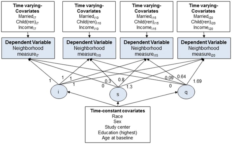
Diagram of Latent Growth Curve model

Variables for person i at time t. α=intercept, β=slope. t=CARDIA exam years 7, 10, 15, 20.

Second, individual characteristics predicting each latent trajectory were added to the model (conditional latent growth curve). The latent intercept and slope were regressed on time-constant covariates (race, sex, baseline age, maximum attained education, and study center) to test if baseline and change over time of each neighborhood measure varied by time-constant characteristics. We hypothesized that blacks live in neighborhoods with less favorable characteristics at baseline, and experience less favorable changes in neighborhood characteristics over time. Other individual characteristics were treated as control variables.

Third, we added time-varying covariates: primary variables of interest were marital and parenthood status (time t) as predictors of each neighborhood measure (time t). Time-varying income was also included in the model. Coefficients for time-varying covariates represent the extent to which the covariate explains deviations from the overall trajectory. We hypothesized that marriage and parenthood would predict higher neighborhood income and lower density of population and amenities.

At each stage, inclusion of higher order terms was evaluated using the BIC. Inclusion of quadratic age or income resulted in small changes to the BIC (>-10) and were omitted from the final models; in one exception, quadratic income was included in the neighborhood poverty model (BIC_diff=-12.9). Absolute measures of model fit [e.g., Comparative Fit Index, Tucker-Lewis Index (Hu and Bentler 1999)] and modification indices are not defined for categorical dependent variables.

In a fourth stage, we tested for interactions with race and sex: race*married, race*child, sex*married, and sex*child at each time period. Interaction analysis was more appropriate than multiple group or stratified analysis because it accommodated the time-variability of marriage and parenthood from one exam period to the next. We used Wald significance of the interaction terms (p<0.05) to assess interactions. To facilitate model symmetry, interaction terms for any given interaction (e.g., race*married) were included for all four time points if significant at any given time point, t. Our approach balanced model parsimony with our interest in identifying potentially important race and sex differences. In adjusted fast food restaurant and public physical activity facility models (Table 4A, 5B; Appendix Table e6), income estimates were fixed to be equal over time to facilitate model convergence.

Table 4.

Table 4A. Coefficients (95% confidence intervals) representing associations of participant sociodemographic characteristics with trajectoriesa of neighborhood fast food restaurant densityb
	Intercept	Slope	Quadratic slope
White (vs. Black)	0.09 (−0.65, 0.84)	−0.13 (−0.95, 0.69)	−0.44 (−1.10, 0.23)
Women (vs. Men)	−0.09 (−0.23, 0.05)	−0.13 (−0.69, 0.42)	0.11 (−0.33, 0.55)
Study Center (vs. Birmingham)
Chicago	−1.00 (−1.25, −0.76)	0.20 (−0.79, 1.18)	−0.53 (−1.30, 0.24)
Minneapolis	−1.13 (−1.36, −0.89)	3.18 (2.21, 4.15)	−2.35 (−3.12, −1.57)
Oakland	−1.13 (−1.35, −0.90)	0.40 (−0.53, 1.32)	0.00 (−0.74, 0.75)
Education (vs. ≤HS)
Some college	0.02 (−0.16, 0.20)	−0.23 (−0.99, 0.53)	0.21 (−0.41, 0.82)
College+	0.27 (0.11, 0.43)	−0.53 (−1.19, 0.13)	0.22 (−0.30, 0.75)
Age at baseline	0.03 (0.01, 0.05)	−0.04 (−0.11, 0.04)	0.02 (−0.04, 0.08)
	Year 7	Year 10	Year 15	Year 20
Marriedd	−0.14 (−0.29, 0.02)	−0.22 (−0.40, −0.05)	−0.32 (−0.51, −0.13)	−0.23 (−0.51, 0.06)
Child(ren) (blacks)d	−0.35 (−0.52, −0.17)	0.64 (0.45, 0.82)	−0.27 (−0.49, −0.06)	−0.22 (−0.57, 0.12)
Child(ren) (whites)d	−0.32 (−0.55, −0.09)	0.10 (−0.14, 0.34)*	−0.18 (−0.45, 0.09)	0.51 (0.11, 0.91)*
Incomee	0.01 (0.00, 0.03)	0.01 (0.00, 0.03)	0.01 (0.00, 0.03)	0.01 (0.00, 0.03)

Table 4B. Coefficients (95% confidence intervals) representing associations of participant sociodemographic characteristics with trajectoriesa of neighborhood supermarket densityb
	Intercept	Slope	Quadratic slope
White (vs. Black)	−0.39 (−0.59, −0.19)	2.08 (1.20, 2.96)	−1.85 (−2.57, −1.13)
Women (vs. Men)	0.00 (−0.15, 0.16)	0.04 (−0.59, 0.67)	−0.09 (−0.58, 0.41)
Study Center (vs. Birmingham)
Chicago	−2.15 (−2.41, −1.89)	3.91 (2.86, 4.97)	−2.76 (−3.60, −1.92)
Minneapolis	−2.08 (−2.36, −1.80)	4.68 (3.61, 5.75)	−3.98 (−4.82, −3.14)
Oakland	−0.66 (−0.93, −0.38)	4.23 (3.18, 5.27)	−3.04 (−3.87, −2.20)
Education (vs. ≤HS)
Some college	0.01 (−0.20, 0.22)	−0.34 (−1.19, 0.52)	0.41 (−0.27, 1.09)
College+	0.05 (−0.13, 0.24)	0.02 (−0.77, 0.81)	0.08 (−0.54, 0.71)
Age at baseline	0.00 (−0.02, 0.03)	0.00 (−0.08, 0.09)	0.02 (−0.05, 0.08)
	Year 7	Year 10	Year 15	Year 20
Married (blacks)d	0.12 (−0.11, 0.34)	−0.11 (−0.35, 0.13)	−0.08 (−0.34, 0.17)	−0.53 (−0.93, −0.13)
Married (whites)d	−0.31 (−0.56, −0.07)*	−0.56 (−0.82, −0.30)*	−0.77 (−1.07, −0.48)*	−0.62 (−1.05, −0.19)
Child(ren)d	−0.18 (−0.35, −0.01)	0.05 (−0.13, 0.22)	−0.25 (−0.44, −0.06)	−0.01 (−0.30, 0.28)
Income	−0.03 (−0.05, −0.01)	0.03 (0.00, 0.05)	0.02 (−0.01, 0.04)	0.02 (−0.02, 0.06)

^aRestricted to CARDIA participants attending at least 2 exams in CARDIA years 7, 10, 15, and 20 (n=4,174). Trajectories estimated using latent growth curve analysis; dependent variables (neighborhood measures) categorized based on observed distribution in the full CARDIA study population, pooling Year 7–20 data. Latent growth curve analysis with categorical dependant variables does not provide absolute model fit indices.

^bResource density (counts per 10,000 population) within 3km Euclidean buffer, categorized into zero and, among non-zero values, tertiles

^cResource density (counts per 100,000 population) within 3km Euclidean buffer, categorized into zero and, among non-zero values, tertiles

^dRace-specific estimated effects of marriage or child(ren) represent (coeff_married + coeff_{married*white}) or (coeff_child + coeff_child*white) in whites, and as coeff_married or coeff_child in blacks. Interaction terms were omitted if Wald p<0.05 at all time points.

^eFixed estimate to be equal over time

^*Interaction p<0.05

Table 5.

Table 5A. Coefficients (95% confidence intervals) representing associations of participant sociodemographic characteristics with trajectoriesa of neighborhood commercial physical activity facility densityb
	Intercept	Slope	Quadratic slope
White (vs. Black)	0.89 (0.69, 1.09)	0.49 (−0.37, 1.35)	−0.31 (−1.01, 0.39)
Women (vs. Men)	−0.13 (−0.27, 0.02)	−0.42 (−1.02, 0.19)	0.14 (−0.33, 0.61)
Study Center (vs. Birmingham)
Chicago	1.79 (1.55, 2.03)	−2.54 (−3.47, −1.61)	1.64 (0.93, 2.35)
Minneapolis	1.65 (1.42, 1.89)	−0.26 (−1.20, 0.69)	0.61 (−0.13, 1.35)
Oakland	1.66 (1.44, 1.88)	0.49 (−0.39, 1.37)	−0.01 (−0.70, 0.67)
Education (vs. ≤HS)
Some college	−0.03 (−0.22, 0.16)	−0.16 (−0.98, 0.66)	0.31 (−0.33, 0.95)
College+	0.38 (0.21, 0.55)	−0.19 (−0.93, 0.54)	0.41 (−0.16, 0.98)
Age at baseline	0.01 (−0.01, 0.03)	−0.05 (−0.13, 0.03)	0.04 (−0.02, 0.10)
	Year 7	Year 10	Year 15	Year 20
Married (blacks)d	−0.36 (−0.57, −0.15)	−0.03 (−0.24, 0.18)	−0.37 (−0.61, −0.12)	−0.28 (−0.62, 0.06)
Married (whites)d	−0.29 (−0.52, −0.05)	−0.48 (−0.72, −0.23)*	−0.28 (−0.58, 0.03)	−0.38 (−0.82, 0.05)
Child(ren)d	−0.27 (−0.43, −0.10)	0.03 (−0.13, 0.18)	−0.21 (−0.40, −0.01)	−0.11 (−0.38, 0.16)
Income	0.03 (0.01, 0.06)	0.02 (−0.01, 0.04)	0.02 (−0.01, 0.05)	0.02 (−0.02, 0.05)

Table 5B. Coefficients (95% confidence intervals) representing associations of participant sociodemographic characteristics with trajectoriesa of neighborhood public physical activity facility densityb
	Intercept	Slope	Quadratic slope
White (vs. Black)	−0.18 (−0.37, 0.02)	−1.03 (−1.91, −0.15)	0.03 (−0.64, 0.71)
Women (vs. Men)	−0.07 (−0.21, 0.07)	−0.34 (−0.94, 0.27)	0.20 (−0.26, 0.67)
Study Center (vs. Birmingham)
Chicago	3.82 (3.57, 4.07)	−2.24 (−3.27, −1.20)	0.80 (0.00, 1.61)
Minneapolis	3.18 (2.92, 3.44)	−0.71 (−1.78, 0.36)	−0.05 (−0.88, 0.79)
Oakland	2.24 (2.01, 2.47)	1.65 (0.65, 2.65)	−1.35 (−2.14, −0.57)
Education (vs. ≤HS)
Some college	−0.05 (−0.24, 0.14)	−0.43 (−1.26, 0.39)	0.33 (−0.32, 0.98)
College+	0.26 (0.10, 0.42)	−1.05 (−1.73, −0.37)	0.65 (0.12, 1.18)
Age at baseline	0.02 (0.00, 0.04)	−0.03 (−0.11, 0.05)	0.02 (−0.04, 0.08)
	Year 7	Year 10	Year 15	Year 20
Marriedd	−0.22 (−0.38, −0.06)	−0.72 (−0.91, −0.53)	−0.57 (−0.78, −0.35)	−0.76 (−1.03, −0.49)
Child(ren) (blacks)d	−0.19 (−0.38, 0.00)	0.49 (0.28, 0.69)	−0.22 (−0.47, 0.03)	−0.57 (−0.92, −0.22)
Child(ren) (whites)d	−0.29 (−0.51, −0.06)	−0.01 (−0.26, 0.25)*	−0.11 (−0.39, 0.17)	0.01 (−0.33, 0.36)*
Incomee	−0.02 (−0.03, 0.00)	−0.02 (−0.03, 0.00)	−0.02 (−0.03, 0.00)	−0.02 (−0.03, 0.00)

^aRestricted to CARDIA participants attending at least 2 exams in CARDIA years 7, 10, 15, and 20 (n=4,174). Trajectories estimated using latent growth curve analysis; dependent variables (neighborhood measures) categorized based on observed distribution in the full CARDIA study population, pooling Year 7–20 data. Latent growth curve analysis with categorical dependant variables does not provide absolute model fit indices.

^bResource density (counts per 10,000 population) within 3km Euclidean buffer, categorized into zero and, among non-zero values, tertiles

^dRace-specific estimated effects of marriage or child(ren) represent (coeff_married + coeff_{married*white}) or (coeff_child + coeff_child*white) in whites, and as coeff_married or coeff_child in blacks. Interaction terms were omitted if Wald p<0.05 at all time points.

^eFixed estimate to be equal over time

^*Interaction p<0.05

Interpretation of model estimates

Latent growth curve analysis of categorical dependent variables calculates trajectories of a latent continuous variable underlying the categorical measures. The predicted trajectory, therefore, approximates changes in a latent standard normal dependent variable over time, with mean intercepts fixed at zero (Masyn, Petras et al. 2014). We interpret the trajectories in terms of direction and shape of the trajectories, but focus on how sociodemographic characteristics are related to the estimated trajectory.

Sensitivity analysis: residential mobility

Observed neighborhood changes can result from one of two mechanisms: through residential relocation of a given participant, or changes in neighborhoods at a given location. For example, neighborhood improvement corresponding to marriage can result from residential relocation to a more advantaged neighborhood, or from remaining in an upwardly mobile neighborhood. To move or remain in the same residential location is a joint decision-making process that likely involves changes within the neighborhood of residence, the degree of discordance between those changes and household preferences and needs, and changes in household financial resources and needs. Isolating one mechanism of neighborhood change ignores the inter-dependence of the decision to relocate or remain in the same neighborhood. Furthermore, residential relocation is in the causal pathway between family structure and neighborhood trajectory, and residential relocation is in itself selective. Therefore, our primary analysis did not condition on residential mobility.

Nevertheless, in sensitivity analyses, we examined the degree to which neighborhood changes corresponding with marital and parenthood status reflected residential mobility, as opposed to changes in characteristics within a given neighborhood. We tested for interactions with residential mobility status (change in residential location between the previous and given exam period): mover*married, mover*child at each time period. As with marriage and parenthood, interaction analysis was used, rather than multi-group or stratified analysis, to accommodate the time-variability of residential relocation.

RESULTS

The study population was approximately 32 years old at baseline (Year 7), with reasonably even distribution by race (black versus white), sex, education, and study center (Table 1). A greater percentage of whites were married throughout the study, with an increasing race difference over time. Percentage with children was greater in blacks than whites early in the study, but increased over time in whites; a decrease in percentage with children from Year 15–20 was observed for whites and blacks. Income increased over time, but was higher in whites than in blacks throughout the time period.

Table 1.

Participant characteristics by race: the Coronary Artery Risk Development in Young Adults (CARDIA) Study, 1992–2011^a

	Black	White
Count	2,038	2,136
Age (baseline) [mean (SE)]b	31.5 (3.8)	32.5 (3.4)
Women (%)	58.39	53.37
Education (%)
≤High school	48.1	25.0
Some college	23.7	13.1
College degree	28.2	61.8
Study Center (%)
Birmingham	26.0	20.4
Chicago	20.8	22.3
Minneapolis	21.2	32.6
Oakland	32.0	24.7
Married (%)
Year 7	35.7	52.9
Year 10	38.3	58.6
Year 15	43.2	62.6
Year 20	43.2	66.1
Child in household (%)
Year 7	56.0	41.1
Year 10	58.0	49.7
Year 15	57.1	57.1
Year 20	48.3	54.5
Income [mean (SE)]
Year 7	4.2 (3.3)	6.5 (4.2)
Year 10	4.3 (3.3)	6.9 (4.1)
Year 15	5.4 (4.0)	8.7 (4.8)
Year 20	5.5 (4.1)	8.5 (4.4)

^aCARDIA participants attending at least 2 exams in CARDIA years 7, 10, 15, and 20

^bAge at baseline for the current analysis (Year 7)

Time-varying individual- and neighborhood-level characteristics exhibited substantial variation across individuals (Table 2; Year 7) and within individuals over time (Table 2, median changes). Between any given pair of exam periods, 14.0–17.4% and 15.0–17.5% of participants changed marital or parenthood status (e.g., percentage who transitioned from married to unmarried, or unmarried to married), respectively; and 40.9–71.4% of participants moved residential locations (Table 2). In the Appendix, we present neighborhood category cutpoints, percentages within each exam year (Appendix Table e3), and percent of participants transitioning among categories across time points (transitioned to lower category, remained in same category, transitioned to higher category; Appendix Table e4).

Overall neighborhood trajectories

In crude neighborhood trajectory models, predicted mean neighborhood poverty and population density exhibited declines over time (Figure 2; Appendix Table e5a), reflecting movement into lower poverty, lower density neighborhoods with age, as well as changes to neighborhood environments. The trajectories were quadratic, reflecting slower declines with a suggestion of a flattening of the trajectory later in the study period.

Figure 2.

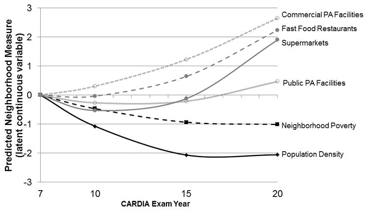
Predicted mean neighborhood trajectories

Crude trajectories; estimated model parameters presented in Appendix Table e4a.

Density of most food and physical activity amenities in neighborhoods where participants lived increased over time; public physical activity facilities exhibited the smallest, but still statistically significant increase. We were able to examine overall trajectories in the full CARDIA sample (without loss to follow-up exclusions) because residential location and, thus, neighborhood measures were available for all surviving CARDIA participants, even if they did not participate in any given exam. Neighborhood trajectories were similar in the analytic and full study samples (Appendix Table e5b), suggesting that study exclusions did not bias the neighborhood trajectories estimated in the analytic sample.

Sociodemographic predictors of neighborhood trajectories

Our primary research question focused on the estimated explanatory value for marriage and parenthood regarding neighborhood trajectories expected based on race, sex, and other time-constant characteristics. We present results from our full models, first discussing time-constant predictors (Tables 3–5).

Table 3.

Table 3A. Coefficients (95% confidence intervals) representing associations of participant sociodemographic characteristics with trajectoriesa of neighborhood population densityb
	Intercept	Slope	Quadratic slope
White (vs. Black)	−1.14 (−1.45, −0.82)	−1.53 (−2.71, −0.34)	0.78 (−0.07, 1.62)
Women (vs. Men)	0.04 (−0.18, 0.25)	−0.39 (−1.11, 0.33)	0.15 (−0.34, 0.64)
Study Center (vs. Birmingham)
Chicago	10.46 (9.90, 11.03)	−8.78 (−10.18, −7.38)	4.85 (3.91, 5.80)
Minneapolis	3.86 (3.55, 4.16)	1.97 (1.06, 2.88)	−1.02 (−1.66, −0.38)
Oakland	5.14 (4.79, 5.49)	1.87 (0.91, 2.82)	−0.95 (−1.61, −0.28)
Education (vs. ≤HS)
Some college	−0.19 (−0.48, 0.10)	−0.60 (−1.59, 0.38)	0.53 (−0.16, 1.22)
College+	−0.24 (−0.49, 0.02)	−0.48 (−1.34, 0.37)	0.52 (−0.07, 1.10)
Age at baseline	0.03 (0.00, 0.06)	0.03 (−0.06, 0.13)	−0.03 (−0.10, 0.03)
	Year 7	Year 10	Year 15	Year 20
Married (blacks)d	−0.34 (−0.66, −0.02)	−0.61 (−0.93, −0.29)	−0.50 (−0.82, −0.17)	−0.82 (−1.18, −0.45)
Married (whites)d	−0.85 (−1.18, −0.52)*	−1.44 (−1.75, −1.13)*	−0.54 (−0.90, −0.17)	−0.98 (−1.32, −0.63)
Child(ren) (blacks)d	−0.07 (−0.37, 0.23)	−0.57 (−0.85, −0.29)	0.13 (−0.17, 0.42)	−0.52 (−0.86, −0.19)
Child(ren) (whites)d	−0.48 (−0.80, −0.16)	−1.16 (−1.46, −0.86)*	−0.62 (−0.95, −0.29)*	−0.67 (−0.98, −0.35)
Income	−0.01 (−0.04, 0.02)	−0.06 (−0.08, −0.03)	−0.03 (−0.06, 0.00)	−0.06 (−0.09, −0.02)

Table 3B. Coefficients (95% confidence intervals) representing associations of participant sociodemographic characteristics with trajectoriesa of neighborhood povertyb
	Intercept	Slope	Quadratic slope
White (vs. Black)	−2.65 (−2.96, −2.34)	0.82 (−0.20, 1.84)	−0.31 (−1.01, 0.40)
Women (vs. Men)	0.10 (−0.10, 0.31)	0.15 (−0.51, 0.81)	−0.13 (−0.58, 0.32)
Study Center (vs. Birmingham)
Chicago	0.33 (0.03, 0.64)	−2.42 (−3.45, −1.38)	1.25 (0.54, 1.96)
Minneapolis	−0.23 (−0.52, 0.07)	−1.42 (−2.31, −0.53)	0.78 (0.16, 1.40)
Oakland	−0.61 (−0.90, −0.31)	−1.50 (−2.38, −0.62)	1.07 (0.46, 1.67)
Education (vs. ≤HS)
Some college	−0.33 (−0.62, −0.03)	−0.15 (−1.08, 0.78)	0.05 (−0.60, 0.70)
College+	−0.89 (−1.13, −0.65)	−0.27 (−1.05, 0.51)	0.06 (−0.47, 0.59)
Age at baseline	0.00 (−0.03, 0.03)	0.03 (−0.06, 0.12)	−0.02 (−0.08, 0.04)
	Year 7	Year 10	Year 15	Year 20
Marriedd	−0.20 (−0.44, 0.04)	−0.46 (−0.68, −0.25)	−0.40 (−0.62, −0.17)	−0.35 (−0.59, −0.11)
Child(ren) (blacks)d	0.21 (−0.10, 0.52)	−0.29 (−0.55, −0.03)	0.11 (−0.18, 0.39)	−0.50 (−0.81, −0.19)
Child(ren) (whites)d	−0.21 (−0.50, 0.08)*	−0.51 (−0.77, −0.26)	−0.67 (−0.93, −0.41)*	−0.58 (−0.85, −0.31)
Income	−0.17 (−0.20, −0.13)	−0.16 (−0.19, −0.13)	−0.20 (−0.24, −0.17)	−0.16 (−0.20, −0.13)
Income2	0.01 (0.00, 0.02)	0.00 (0.00, 0.01)	0.01 (0.01, 0.02)	0.01 (0.00, 0.01)

^aRestricted to CARDIA participants attending at least 2 exams in CARDIA years 7, 10, 15, and 20 (n=4,174). Trajectories estimated using latent growth curve analysis; dependent variables (neighborhood measures) categorized based on observed distribution in the full CARDIA study population, pooling Year 7–20 data. Latent growth curve analysis with categorical dependant variables does not provide absolute model fit indices.

^bPersons per square mile within 1km Euclidean buffer, categorized into quintiles

^cProportion households <150% of poverty within census tract (1990 and 2000 U.S. Census for CARDIA years 7 & 10 and 15 & 20, respectively), categorized into quintiles

^dRace-specific estimated effects of marriage or child(ren) represent (coeff_married + coeff_{married*white}) or (coeff_child + coeff_child*white) in whites, and as coeff_married or coeff_child in blacks. Interaction terms were omitted if Wald p<0.05 at all time points.

^*Interaction p<0.05

Time-constant predictors

Compared to blacks, whites lived in neighborhoods with lower poverty, population density, and density of supermarkets, and higher density of commercial physical activity facilities at Year 7 (estimated effect of white race on Intercepts in Tables 3–5). There was no baseline race difference in fast food restaurant density or public physical activity facility. White race was a significant predictor of deviations from the overall trajectory of population density (more negative slope), supermarket density (weaker upward quadratic slope), and public physical activity density (less negative slope) although the curves were substantively similar over time (graph not shown). Race differences in slopes and quadratic slopes of other neighborhood characteristics were not observed. Deviations from neighborhood trajectories were similar in men and women. There was variation by study center, education, and baseline age.

Time-varying predictors: marriage and parenthood

At any given time point, participants who were married lived in neighborhoods with lower population density, poverty, and density of most amenities than expected from the overall trajectory (Tables 3–5). Associations between marriage and population density, supermarkets, and commercial physical activity facilities were generally stronger and more consistent in whites than in blacks (interaction p<0.05 for at least one time point). Estimated effects of parenthood were similar but weaker and less consistent across neighborhood characteristics than estimated effects of marriage. Associations between parenthood and population density and neighborhood poverty were stronger for whites than blacks (interaction p<0.05 for at least one time point). Interactions between race and parenthood were also observed for fast food restaurants and public physical activity density, but these were less consistent in significance and direction across time points.

Residential relocation

In general, associations between marital and parenthood status and neighborhood characteristics (time t) were stronger among participants who moved between the previous and concurrent CARDIA exam (between time t-1 and t) (interaction p<0.05; Appendix Table e6). Interactions between marital status and residential mobility were significant for all neighborhood characteristics, while interactions between parenthood and residential mobility were significant only for population density, neighborhood poverty, and public physical activity facilities. Associations between marital or parenthood status on neighborhood characteristics were typically stronger but in the same direction in movers than in non-movers.

DISCUSSION

Using sociodemographic and neighborhood environment data on a large cohort of black and white young adults followed over 13 years, we conducted the first investigation of how marriage and parenthood are related to aspects of the neighborhood environment that are relevant to obesity prevention. Despite living in higher income neighborhoods, married participants and parents tended to live in lower density neighborhoods with fewer amenities. These neighborhoods had lower availability of amenities linked with healthy (supermarkets, commercial and public physical activity facilities) as well as unhealthy (fast food restaurants) behaviors or body weight in this study population (Boone-Heinonen, Gordon-Larsen et al. 2011; Boone-Heinonen, Diez-Roux et al. 2013). Notably, associations of marriage and parenthood with neighborhood trajectories were more pronounced in whites than in blacks. These findings have implications for targeted interventions for young adults and their families and for methodological aspects of neighborhood health research.

Parallel changes in multiple neighborhood characteristics over time

Our overall findings emphasize the complexity involved in urban design, housing costs, and residential decisions. Consistent with well-recognized urban design concepts (Cervero and Kockelman 1997), measures of neighborhood density generally tracked together: population density and density of amenities of all types. Notably, amenities considered to be “healthy” and “unhealthy” exhibited similar trajectories over time and were predicted by similar participant sociodemographic characteristics. This finding suggests that changes in neighborhood environments generally occur with regard to density of population and all types of amenities, rather than specific types of amenities changing more than others. Yet, neighborhood poverty decreased over time in parallel with declines in neighborhood density. Our findings may reflect age-related increases in preference for larger housing, which tends to be more available and affordable in lower density areas, ease of transportation, or safety. These temporal patterns may also reflect secular trends in retail and urban planning.

Furthermore, these parallel neighborhood changes likely also occur with respect to unmeasured characteristics such as public transport, school quality, and childcare facilities. These findings underscore the difficulty of distinguishing independent effects of discrete neighborhood aspects and the need for holistic conceptualization of neighborhoods. Recent work using composite neighborhood measures begins to address these complexities (Wall, Larson et al. 2012; Meyer, Boone-Heinonen et al. 2015). However, composite measures should be balanced with the public health objective of identifying specific, policy-relevant neighborhood modifications most likely to improve population health.

Associations of marriage and parenthood with neighborhood trajectories

We observed substantial changes in marriage and parenthood status, residential mobility, and neighborhood change during the study period, which followed adults throughout their thirties and early forties. At any given time point, marriage was strongly associated with neighborhood characteristics. Marriage was associated with lower neighborhood poverty, consistent with resource consolidation and stability that occur with marriage (Vespa and Painter 2011). We also found that marriage was associated with lower neighborhood density. These findings suggest that living outside of the urban core might be preferable to married couples (Walker and Li 2007), perhaps due to residential preferences for larger housing and lot size or higher safety. Conversely, those who live in less densely populated areas may be more likely to be married.

In comparison to marital status, parenthood was not as strongly or consistently associated with neighborhood characteristics. In particular, parenthood was weakly or unrelated to density of neighborhood amenities. This finding is consistent with evidence that among households with children, housing costs and type are more important than access to neighborhood amenities in housing decisions (Lund 2006). Likewise, other factors such as school quality (Black and Machin 2011), child care facilities, lot size, or other amenities such as playgrounds may be stronger drivers of residential preferences among parents. Another explanation is that residential decisions related to parenting may have occurred after marriage, in anticipation of children.

Associations of race and socioeconomic indicators with neighborhood trajectories

Furthermore, marriage and parenthood were stronger and more consistent predictors of neighborhood characteristics in whites than in blacks. This race difference may reflect a number of processes. In particular, our descriptive data suggest that black participants tended to become parents earlier than whites, but were less likely to be married. That is, any residential mobility tied to parenthood may have occurred prior to the study period to a greater extent in blacks than whites, and marriage may less adequately measure commitment tied to residential decisions in blacks. However, cohabitation was uncommon in our study (0–1% in Years 7 and 10, 6–7% in Year 15 and 20) and similar by race. Second, social ties to individuals living in higher density areas (Dawkins 2006) or social barriers to moving into lower density areas (Charles 2000) may be stronger in blacks than in whites. Third, compared to family structure, other racially patterned factors such as reliance on public transportation or public services in urban centers may be stronger drivers of residential decisions (Glaeser, Kahn et al. 2008).

In addition to modifying associations between marriage and parenthood and neighborhood characteristics, race was the most consistent predictor of neighborhood trajectories. Whites lived in neighborhoods with lower poverty and population density in the first time period; the race difference in population density was constant over time. This finding is consistent with a large body of research on residential segregation and residential mobility (Jackson and Mare 2007; Keels 2008; Timberlake 2009; Silver, Weitzman et al. 2012). Our study contributes to this literature by examining longitudinal residential patterns in the context of obesity-related aspects of the neighborhood built environment. We found race differences in food and physical activity amenities at baseline (year 7), but these race differences were substantively consistent over time. These findings suggest that racial differences in neighborhood environments are established in young adulthood.

While racial minorities face inadequate access to healthy neighborhood amenities in many geographic areas (Baker, Schootman et al. 2006; Moore, Diez Roux et al. 2008; Bodor, Ulmer et al. 2010), we found that black adults lived in neighborhoods with greater density of supermarkets and public physical activity facilities. This finding contrasts with evidence of poorer diet and lower physical activity (Ham and Ainsworth 2010; Kirkpatrick, Dodd et al. 2012) and lower perceived access to food and physical activity amenities (Walker, Keane et al. 2010) in blacks compared to whites. Yet it is consistent with other research that emphasizes the importance of quality, affordability, and cultural sensitivity in shaping accessibility to neighborhood amenities (Black, Ntani et al. 2012; Caspi, Sorensen et al. 2012), but that are not captured in our neighborhood measures. Clearly, better understanding of the joint and interactive estimated effects of the built environment, detailed aspects of access, and social factors on obesity-related behavior is needed.

In an illustrative exception, despite greater density of population and most amenities, blacks lived in neighborhoods with a lower density of commercial physical activity facilities. Such facilities require per-use costs or paid memberships; business decisions about their geographic location may be particularly sensitive to local demand and financial resources.

Implications for the role of neighborhood environments in marriage- and parenthood-related weight gain

Our finding that families tend to live in higher income, lower density neighborhoods supports our hypothesis that families prioritize larger, higher quality housing, higher school quality, or ease of transportation in residential decisions. We posed this hypothesis within a framework conceptualizing these practical barriers to living in health-promoting neighborhoods as potential contributors to adverse changes in diet, physical activity, and body weight observed with marriage and parenthood (Jeffery and Rick 2002; Ortega, Brown et al. 2011; Bassett-Gunter, Levy-Milne et al. 2013). While we did not examine behavioral or health outcomes in this study, our findings provide insight about environmental determinants of marriage- and parenthood-related weight gain.

Marriage- and parenthood-related neighborhood differences were strongest in whites, who tend to exhibit weaker associations between neighborhood characteristics and health behaviors or outcomes (Diez Roux, Evenson et al. 2007; Boone-Heinonen, Diez Roux et al. 2011). That is, residential change is most responsive to marriage and parenthood in those least vulnerable to adverse influences of neighborhoods on health. Rather, among whites or other subpopulations with greater social or economic advantage, family factors such as time constraints (Bauer, Hearst et al. 2012) may be stronger contributors to marriage- and parenthood differences in obesity-related health. Therefore, our findings do not support the idea that neighborhood environments contribute to marriage- and parenthood-related weight gain. They do, however, emphasize that the relative influences of neighborhood versus family environments are unknown, likely dynamic, and vary by race and socioeconomic subgroup. Future research studying neighborhood and family environmental determinants should also seek to identify aspects of marriage and parenthood of most importance to health-related behavior.

Implications for residential self-selection bias

Methodologically, knowledge about correlates of neighborhood patterns over time can help to quantify and address residential self-selection bias in studies estimating effects of neighborhood features on obesity or related behaviors. In our study, we selected sociodemographic characteristics known to be strongly related to obesity-related behaviors and outcomes, then examined how they were associated with neighborhood trajectories. Our findings indicate that race, marital status, and parenthood are important correlates of neighborhood trajectories. However, our findings also suggest that changes in neighborhood environments occur in parallel with overall density, as opposed to specific types of amenities or design features of interest to obesity research. Therefore, it is unlikely that bias in the estimated effects of neighborhood characteristics on health results from location selectivity of specific types of neighborhood amenities. Rather, more critical steps toward advancing our understanding of specific aspects of neighborhoods that impact obesity-related health include (a) improvement in neighborhood measures to more fully account for overall neighborhood design and (b) improvement in statistical methodology and study design to address the systematic differences in residential mobility patterns by race and family structure.

Residential mobility

Associations between marital and parenthood status and neighborhood change were generally stronger in movers than in non-movers. This finding suggests that the marriage- and parenthood-related neighborhood differences observed in our primary analysis most strongly reflect neighborhood change occurring as a result of residential mobility. However, significant associations between marital or parenthood status and most neighborhood characteristics were also observed among non-movers, suggesting that residential stability within changing neighborhood environments is also important.

Overall, these findings suggest that drivers of neighborhood change may operate either through residential mobility, or through remaining in a neighborhood undergoing change. This finding supports our rationale for focusing on neighborhood change resulting from either mechanism. Residential relocation and stability stem from the same decision making process that leads to a neighborhood consistent with each family’s financial resources balanced with resource needs. Marriage may prompt relocation into a wealthier neighborhood or enhance the ability to remain in an upwardly mobile neighborhood; either process can offer health benefits. Furthermore, conditioning on the mediating variable (residential relocation) may introduce bias from unmeasured variables associated with both residential relocation and neighborhood change. For example, home owners may be more likely to remain in the same home, as well as live in a neighborhood with a higher proportion of home owners, which is predictor of higher property values (Rohe and Stewart 2010). Other approaches, such as simultaneous modeling of residential mobility, are needed to understand drivers of residential stability versus relocation in the context of changing household structure and resources throughout the life course, evolving neighborhood characteristics, and social contexts.

Limitations and Strengths

Our findings are based on observational data, thus causality may not be inferred, rather it may be suggested. Granted, our time-variant modeling approach lends some credence to suggestions regarding direction of causality, but the complexity of causal relationships likely is not fully captured in our models. Our analytic approach examined within- and between-person variability in family structure that was associated from establishment, dissolution, or maintenance of marriage or parenthood. For example, lower population density corresponding with new marriage and higher population density corresponding with marriage dissolution contributed to the model equivalently. Other approaches that distinguish these processes may provide important insights, but were not appropriate with our growth trajectory approach, and requires a larger study population with greater numbers of marriage and parenthood transitions. Future research in larger study populations can explore neighborhood changes related to having greater numbers of children of different ages, as well as interactive relationships with parent age.

Exclusion of participants with more than two missing CARDIA exams was necessary for the growth curve analysis, but was overrepresented by sociodemographic subgroups that are typically difficult to track over time. Therefore, selection bias may have contributed to the observed findings, but we showed that overall neighborhood trajectories were similar for the total study population compared to those included in the current study.

Our measures of the food retail and physical activity environments were based on commercial amenity data that contain error. Validation studies suggest that count error does not vary by neighborhood- or individual-level sociodemographics, but we did not examine differences in qualitative aspects of neighborhood amenities that vary across by neighborhood wealth. Whether salient geographic scales differ for marriage- or parenthood-related residential decisions versus health-related outcomes is a useful topic for future research. Dun & Bradstreet is the only data source that provides historical data back to the baseline period (1984) that is comparable across the U.S., thus enabling our unique examination of residential patterns over 13 years. Estimated neighborhood trajectories could reflect changes in coding or completeness of Dun & Bradstreet data over time; however, our main research questions concerned predictors of these trajectories, and systematic differences in coding or completeness with respect to these predictors is unlikely.

These limitations are balanced with our comparable, objective, and time-varying data on a wide range of socioeconomic and built environment characteristics in a large, diverse sample of young adults residing throughout the U.S. and followed into middle age.

Conclusions

Over 13 years of follow-up from young to middle adulthood, those who were married or had children tended to live in higher income, yet lower density neighborhoods than those who were unmarried or without children. Married participants and parents had lower availability of all types of neighborhood amenities, including both “healthy” and “unhealthy”, but these patterns were stronger in whites than in blacks. Our findings suggest that neighborhood selection is not based on specific neighborhood amenities, but rather on more general aspects of density, price, and characteristics of specific homes. Greater understanding of interactive family and neighborhood environmental barriers to healthy living among families is critical for developing strategies for preventing weight gain and retention throughout the life course.

HIGHLIGHTS.

• We estimated effects of family structure on obesity-related neighborhood changes.

• Marriage and parenthood were associated with living in wealthier neighborhoods.

• Families tended to live in neighborhoods with few food and physical activity amenities.

• Neighborhood-family structure associations were stronger in whites than blacks.

References

- Averett SL, Sikora A, et al. For better or worse: relationship status and body mass index. Econ Hum Biol. 2008;6(3):330–349. doi: 10.1016/j.ehb.2008.07.003. [DOI] [PubMed] [Google Scholar]
- Baker EA, Schootman M, et al. The role of race and poverty in access to foods that enable individuals to adhere to dietary guidelines. Prev Chronic Dis. 2006;3(3):A76. [PMC free article] [PubMed] [Google Scholar]
- Bassett-Gunter RL, Levy-Milne R, et al. Oh baby! Motivation for healthy eating during parenthood transitions: a longitudinal examination with a theory of planned behavior perspective. Int J Behav Nutr Phys Act. 2013;10:88. doi: 10.1186/1479-5868-10-88. [DOI] [PMC free article] [PubMed] [Google Scholar]
- Bauer KW, Hearst MO, et al. Parental employment and work-family stress: Associations with family food environments. Soc Sci Med. 2012;75(3):496–504. doi: 10.1016/j.socscimed.2012.03.026. [DOI] [PMC free article] [PubMed] [Google Scholar]
- Bellows-Riecken KH, Rhodes RE. A birth of inactivity? A review of physical activity and parenthood. Prev Med. 2008;46(2):99–110. doi: 10.1016/j.ypmed.2007.08.003. [DOI] [PubMed] [Google Scholar]
- Black C, Ntani G, et al. Variety and quality of healthy foods differ according to neighbourhood deprivation. Health Place. 2012;18(6):1292–1299. doi: 10.1016/j.healthplace.2012.09.003. [DOI] [PMC free article] [PubMed] [Google Scholar]
- Black SE, Machin S. Housing Valuations of School Performance. Handbook of the Economics of Education. 2011;3:485–519. [Google Scholar]
- Blake CE, Wethington E, et al. Behavioral contexts, food-choice coping strategies, and dietary quality of a multiethnic sample of employed parents. J Am Diet Assoc. 2011;111(3):401–407. doi: 10.1016/j.jada.2010.11.012. [DOI] [PMC free article] [PubMed] [Google Scholar]
- Bodor JN, V, Ulmer M, et al. The rationale behind small food store interventions in low-income urban neighborhoods: insights from New Orleans. J Nutr. 2010;140(6):1185–1188. doi: 10.3945/jn.109.113266. [DOI] [PMC free article] [PubMed] [Google Scholar]
- Boker SM. Differential Equation Models for Longitudinal Data. In: Mendard S, editor. Handbook of Longitudinal Research. New York: Elsevier; 2007. pp. 639–652. [Google Scholar]
- Bollen KA, Curran PJ. Latent Curve Models: A Structural Equation Perspective. Hoboken, NJ: John Wiley & Sons; 2006. [Google Scholar]
- Boone-Heinonen J, Diez-Roux AV, et al. The Neighborhood Energy Balance Equation: Does Neighborhood Food Retail Environment + Physical Activity Environment = Obesity? The CARDIA Study. PLoS One. 2013;8(12):e85141. doi: 10.1371/journal.pone.0085141. [DOI] [PMC free article] [PubMed] [Google Scholar]
- Boone-Heinonen J, Diez Roux AV, et al. Neighborhood socioeconomic status predictors of physical activity through young to middle adulthood: The CARDIA study. Soc Sci Med. 2011;72(5):641–649. doi: 10.1016/j.socscimed.2010.12.013. [DOI] [PMC free article] [PubMed] [Google Scholar]
- Boone-Heinonen J, Evenson KR, et al. Built and socioeconomic environments: patterning and associations with physical activity in U.S. adolescents. Int J Behav Nutr Phys Act. 2010;7:45. doi: 10.1186/1479-5868-7-45. [DOI] [PMC free article] [PubMed] [Google Scholar]
- Boone-Heinonen J, Gordon-Larsen P, et al. Fast Food Restaurants and Food Stores: Longitudinal Associations With Diet in Young to Middle-aged Adults: The CARDIA Study. Arch Intern Med. 2011;171(13):1162–1170. doi: 10.1001/archinternmed.2011.283. [DOI] [PMC free article] [PubMed] [Google Scholar]
- Boone-Heinonen J, Popkin BM, et al. What neighborhood area captures built environment features related to adolescent physical activity? Health Place. 2010;16(6):1280–1286. doi: 10.1016/j.healthplace.2010.06.015. [DOI] [PMC free article] [PubMed] [Google Scholar]
- Brown H, Roberts J. Exercising choice: the economic determinants of physical activity behaviour of an employed population. Soc Sci Med. 2011;73(3):383–390. doi: 10.1016/j.socscimed.2011.06.001. [DOI] [PMC free article] [PubMed] [Google Scholar]
- Byrne BM. Structural Equation Modeling with Mplus: Basic Concepts, Applications, and Programming. New York: Routledge; 2012. [Google Scholar]
- Caspi CE, Sorensen G, et al. The local food environment and diet: a systematic review. Health Place. 2012;18(5):1172–1187. doi: 10.1016/j.healthplace.2012.05.006. [DOI] [PMC free article] [PubMed] [Google Scholar]
- Cervero R, Kockelman K. Travel demand and the 3Ds: Density, diversity, and design. Transportation Research Part D-Transport and Environment. 1997;2(3):199–219. [Google Scholar]
- Charles CZ. Neighborhood racial-composition preferences: Evidence from a multiethnic metropolis. Social Problems. 2000;47(3):379–407. [Google Scholar]
- Clark WAV, Withers SD. Family migration and mobility sequences in the United States: spatial mobility in the context of the life course. Demographic Research. 2007;17:591–622. [Google Scholar]
- Cooke TJ. Migration in a family way. Population Space and Place. 2008;14(4):255–265. [Google Scholar]
- D&B (Dun & Bradstreet) D&B’s Data Quality. Available at: http://www.dnb.com/company/our-data/data-quality-of-data-as-a-service.html. Retrieved May 17, 2013.
- Dawkins CJ. Are social networks the ties that bind families to neighborhoods? Housing Studies. 2006;21(6):867–881. [Google Scholar]
- Diez Roux AV, Evenson KR, et al. Availability of recreational resources and physical activity in adults. Am J Public Health. 2007;97(3):493–499. doi: 10.2105/AJPH.2006.087734. [DOI] [PMC free article] [PubMed] [Google Scholar]
- DOL (U.S. Department of Labor) Consumer Price Index. Available at: http://www.bls.gov/cpi/. Retrieved May 17, 2013.
- DOL (U.S. Department of Labor) SIC Manual. Available at: http://www.osha.gov/pls/imis/sic_manual.html. Retrieved May 17, 2013.
- Edvardsson K, Ivarsson A, et al. Giving offspring a healthy start: parents’ experiences of health promotion and lifestyle change during pregnancy and early parenthood. BMC Public Health. 2011;11:936. doi: 10.1186/1471-2458-11-936. [DOI] [PMC free article] [PubMed] [Google Scholar]
- Feng J, Glass TA, et al. The built environment and obesity: a systematic review of the epidemiologic evidence. Health Place. 2010;16(2):175–190. doi: 10.1016/j.healthplace.2009.09.008. [DOI] [PubMed] [Google Scholar]
- Glaeser EL, Kahn ME, et al. Why do the poor live in cities? The role of public transportation. J Urban Econ. 2008;63:1–24. [Google Scholar]
- Gunderson EP, Murtaugh MA, et al. Excess gains in weight and waist circumference associated with childbearing: The Coronary Artery Risk Development in Young Adults Study (CARDIA) Int J Obes Relat Metab Disord. 2004;28(4):525–535. doi: 10.1038/sj.ijo.0802551. [DOI] [PMC free article] [PubMed] [Google Scholar]
- Ham SA, Ainsworth BE. Disparities in data on Healthy People 2010 physical activity objectives collected by accelerometry and self-report. Am J Public Health. 2010;100(Suppl 1):S263–268. doi: 10.2105/AJPH.2009.180075. [DOI] [PMC free article] [PubMed] [Google Scholar]
- Hou N, Popkin BM, et al. Longitudinal associations between neighborhood-level street network with walking, bicycling, and jogging: the CARDIA study. Health Place. 2010;16(6):1206–1215. doi: 10.1016/j.healthplace.2010.08.005. [DOI] [PMC free article] [PubMed] [Google Scholar]
- Hu L-t, Bentler PM. Cutoff criteria for fit indexes in covariance structure analysis: Conventional criteria versus new alternatives. Structural Equation Modeling. 1999;6:1–55. [Google Scholar]
- Hughes GH, Cutter G, et al. Recruitment in the Coronary Artery Disease Risk Development in Young Adults (Cardia) Study. Control Clin Trials. 1987;8(4 Suppl):68S–73S. doi: 10.1016/0197-2456(87)90008-0. [DOI] [PubMed] [Google Scholar]
- Jackson MI, Mare RD. Cross-sectional and longitudinal measurements of neighborhood experience and their effects on children. Social Science Research. 2007;36(2):590–610. doi: 10.1016/j.ssresearch.2007.02.002. [DOI] [PMC free article] [PubMed] [Google Scholar]
- Jeffery RW, Rick AM. Cross-sectional and longitudinal associations between body mass index and marriage-related factors. Obes Res. 2002;10(8):809–815. doi: 10.1038/oby.2002.109. [DOI] [PubMed] [Google Scholar]
- Kahn HS, Williamson DF. The contributions of income, education and changing marital status to weight change among US men. Int J Obes. 1990;14(12):1057–1068. [PubMed] [Google Scholar]
- Keels M. Residential attainment of now-adults Gautreaux children: do they gain, hold, or lose ground in neighborhood ethnic and economic segregation? Housing Studies. 2008;23(4):541–564. [Google Scholar]
- Kestens Y, Daniel M. Social inequalities in food exposure around schools in an urban area. Am J Prev Med. 2010;39(1):33–40. doi: 10.1016/j.amepre.2010.03.014. [DOI] [PubMed] [Google Scholar]
- Kirkpatrick SI, Dodd KW, et al. Income and race/ethnicity are associated with adherence to food-based dietary guidance among US adults and children. J Acad Nutr Diet. 2012;112(5):624–635. e626. doi: 10.1016/j.jand.2011.11.012. [DOI] [PMC free article] [PubMed] [Google Scholar]
- Lund H. Reasons for living in a transit-oriented development, and associated transit use. J Am Plan Assn. 2006;72(3):357–366. [Google Scholar]
- Masyn KE, Petras H, et al. Growth curve models with categorical outcomes. In: Bruinsma G, Weisburd D, editors. Encyclopedia of Criminology and Criminal Justice. New York: Springer; 2014. 2013–2025. [Google Scholar]
- Meyer KA, Boone-Heinonen J, et al. Combined measure of neighborhood food and physical activity environments and weight-related outcomes: The CARDIA study. Health Place. 2015;33C:9–18. doi: 10.1016/j.healthplace.2015.01.004. [DOI] [PMC free article] [PubMed] [Google Scholar]
- Michielin F, Mulder CH, et al. Distance to parents and geographical mobility. Population Space and Place. 2008;14(4):327–345. [Google Scholar]
- Moore LV, Diez Roux AV, et al. Availability of recreational resources in minority and low socioeconomic status areas. Am J Prev Med. 2008;34(1):16–22. doi: 10.1016/j.amepre.2007.09.021. [DOI] [PMC free article] [PubMed] [Google Scholar]
- Mulder CH. The family context and residential choice: A challenge for new research. Population Space and Place. 2007;13(4):265–278. [Google Scholar]
- Muthen and Muthen. MPlus. 2011 Available at: http://www.statmodel.com/index.shtml.
- Ortega FB, Brown WJ, et al. In fitness and health? A prospective study of changes in marital status and fitness in men and women. Am J Epidemiol. 2011;173(3):337–344. doi: 10.1093/aje/kwq362. [DOI] [PMC free article] [PubMed] [Google Scholar]
- Papas MA, Alberg AJ, et al. The built environment and obesity. Epidemiol Rev. 2007;29:129–143. doi: 10.1093/epirev/mxm009. [DOI] [PubMed] [Google Scholar]
- Richardson AS, Boone-Heinonen J, et al. Neighborhood fast food restaurants and fast food consumption: a national study. BMC Public Health. 2011;11:543. doi: 10.1186/1471-2458-11-543. [DOI] [PMC free article] [PubMed] [Google Scholar]
- Rohe WM, Stewart LS. Homeownership and neighborhood stability. Housing Policy Debate. 2010;7(1):1996. [Google Scholar]
- Scharoun-Lee M, Kaufman JS, et al. Obesity, race/ethnicity and life course socioeconomic status across the transition from adolescence to adulthood. J Epidemiol Community Health. 2009;63(2):133–139. doi: 10.1136/jech.2008.075721. [DOI] [PMC free article] [PubMed] [Google Scholar]
- Silver D, Weitzman BC, et al. How residential mobility and school choice challenge assumptions of neighborhood place-based interventions. Am J Health Promot. 2012;26(3):180–183. doi: 10.4278/ajhp.100326-ARB-97. [DOI] [PubMed] [Google Scholar]
- Sobal J, Rauschenbach BS, et al. Marital status, fatness and obesity. Soc Sci Med. 1992;35(7):915–923. doi: 10.1016/0277-9536(92)90106-z. [DOI] [PubMed] [Google Scholar]
- The NS, Gordon-Larsen P. Entry into romantic partnership is associated with obesity. Obesity (Silver Spring) 2009;17(7):1441–1447. doi: 10.1038/oby.2009.97. [DOI] [PMC free article] [PubMed] [Google Scholar]
- Timberlake JM. “Scratchin’ and Surviving” or “Movin’ on Up?” Two Sources of Change in Children’s Neighborhood SES. Population Research and Policy Review. 2009;28(2):195–219. [Google Scholar]
- U.S Census Bureau. Geographic Terms and Concepts - Block Groups. Available at: http://www.census.gov/geo/reference/gtc/gtc_bg.html. Retrieved May 17, 2013.
- U.S. Census Bureau. How the Census Bureau Measures Poverty. 2009 Sep 29; Retrieved March 19, 2010, from http://www.census.gov/hhes/www/poverty/povdef.html.
- Umberson D, Liu H, et al. Parenthood and trajectories of change in body weight over the life course. Soc Sci Med. 2011;73(9):1323–1331. doi: 10.1016/j.socscimed.2011.08.014. [DOI] [PMC free article] [PubMed] [Google Scholar]
- Vespa J, Painter MA., 2nd Cohabitation history, marriage, and wealth accumulation. Demography. 2011;48(3):983–1004. doi: 10.1007/s13524-011-0043-2. [DOI] [PubMed] [Google Scholar]
- Walker JL, Li J. Latent lifestyle preferences and household location decisions. J Geograph Syst. 2007;9:977–101. [Google Scholar]
- Walker RE, Keane CR, et al. Disparities and access to healthy food in the United States: A review of food deserts literature. Health Place. 2010;16(5):876–884. doi: 10.1016/j.healthplace.2010.04.013. [DOI] [PubMed] [Google Scholar]
- Wall MM, Larson NI, et al. Patterns of obesogenic neighborhood features and adolescent weight: a comparison of statistical approaches. Am J Prev Med. 2012;42(5):e65–75. doi: 10.1016/j.amepre.2012.02.009. [DOI] [PMC free article] [PubMed] [Google Scholar]
Associated Data
This section collects any data citations, data availability statements, or supplementary materials included in this article.