Comparative investigation of the energetic ion spectra comprising the magnetospheric ring currents of the solar system

Abstract

Investigated here are factors that control the intensities and shapes of energetic ion spectra that make up the ring current populations of the strongly magnetized planets of the solar system, specifically those of Earth, Jupiter, Saturn, Uranus, and Neptune. Following a previous and similar comparative investigation of radiation belt electrons, we here turn our attention to ions. Specifically, we examine the possible role of the differential ion Kennel-Petschek limit, as moderated by Electromagnetic Ion Cyclotron (EMIC) waves, as a standard for comparing the most intense ion spectra within the strongly magnetized planetary magnetospheres. In carrying out this investigation, the substantial complexities engendered by the very different ion composition distributions of these diverse magnetospheres must be addressed, given that the dispersion properties of the EMIC waves are strongly determined by the ion composition of the plasmas within which the waves propagate. Chosen for comparison are the ion spectra within these systems that are the most intense observed, specifically at 100 keV and 1 MeV. We find that Earth and Jupiter are unique in having their most intense ion spectra likely limited and sculpted by the Kennel-Petschek process. The ion spectra of Saturn, Uranus, and Neptune reside far below their respective limits and are likely limited by interactions with gas and dust (Saturn) and by the absence of robust ion acceleration processes (Uranus and Neptune). Suggestions are provided for further testing the efficacy of the differential Kennel-Petschek limit for ions using the Van Allen Probes.

1. Introduction

What criterion or standard do we use when comparing the particle populations within the highly diverse magnetospheres of the solar system? Should a planet that is 10 times bigger or that has a magnetic field that is 10 times stronger have energetic particle populations that are 10 times more intense or 10 times more energetic? For relativistic electron spectra of the strongly magnetized planets of the solar system, one answer has been suggested and supported. Specifically, following the pioneering work of Kennel and Petschek [1966], Schulz and Davidson [1988], Davidson et al. [1988], and Summers et al. [2009], Mauk and Fox [2010] developed a general approach to evaluating a relativistic differential Kennel-Petschek (KP) limit for energetic magnetospheric electrons that successfully provides a standard for comparing the relativistic electron radiation belts of all of the strongly magnetized planets of the solar system. The electron KP limit makes use of the expected runaway growth of whistler waves under certain conditions and the associated strong scattering of electrons into the magnetic loss cone. This work also confirmed for the relativistic regime the nonrelativistic Schulz and Davidson [1988] prediction of a characteristic E⁻¹ shape of the spectra for energies <1 MeV. It was found specifically that for Earth, Jupiter, and Uranus, the electron spectra are pegged close to the KP limit between 0.1 and 1 MeV and that the spectra are characterized by the ∽ E⁻¹ shape within the same range of energy. At higher energies the spectra are below the corresponding KP limits. Neptune and Saturn were shown to be different. Neptune achieves the limit only close to the 0.1 MeV energy, and it is suggested that the energization processes are not robust enough to challenge the KP limit at energies as high as 1 MeV. At Saturn the spectra fall well below the limit for all energies, at least during the Cassini mission epoch, and it is suggested that the Saturnian spectra are strongly degraded by the unique gas and dust populations within that system.

The present work is a companion to that earlier work on electrons. Here we consider the question of the limiting factors for the energetic ion spectra that comprise the ring current populations of the five planetary magnetospheres. Primarily by means of the mechanism of the diamagnetic current that arises from particle pressure gradients, these populations carry major fractions of the electric currents that encircle these planets in the inner to middle regions and distort the magnetic field shapes somewhat away from their dipolar configurations. Here we develop for ions the differential Kennel-Petschek limit as a standard for comparing the intensities and spectral shapes. For ions, the electromagnetic ion cyclotron (EMIC) waves are thought to play the role that whistler waves play for electrons. The analysis provided here is performed in a fashion that accommodates the complexities of the multispecies composition of the plasmas that determine the properties of the EMIC waves. This examination has already been carried out for the case of Earth in Mauk [2013] where it was found that the proton spectra reside somewhat above the classical KP limit for energies <100 keV by a roughly consistent amount. The observed flat spectral shapes also may correspond to the spectral sculpting that is expected with the KP process. Here we expand that examination to all of the other strongly magnetized planets of the solar system. We note here that there are other processes that likely play a role in the general loss of energetic ions, but under appropriate conditions the EMIC moderated scattering losses have the potential to be much faster than other processes that have been invoked [Daglis et al., 1999; Erlandson and Ukhorskiy, 2001]. At Earth, for example, collisional processes such as charge exchange are not fast enough to explain the initial rapid storm recovery phase [e.g., Keika et al., 2006].

2. Planetary Ion Spectra

The ion spectra that we will be examining are shown in Figure1. Here are fits to spectra that are the most intense recorded in the literature for the ring current regions of our five target planets. Specifically, they are the most intense at one of two energies, 100 keV and 1 MeV, or both. The solid line spectra are protons (or inferred to be protons based on the characteristics of the measurement techniques) and the dashed lines are heavy ions; oxygen for Earth, sulfur or sulfur/oxygen for Jupiter, and water group ions for Saturn. The fitting function is described in the next section. The literature sources for the spectra and the fitting parameters are provided in Table1.

Figure 1.

Energetic ion spectra sampled within the ring current regions of the five strongly magnetized planets of the solar system and fitted with equation (3). The spectra are the most intense observed within these systems specifically at 100 keV and 1 MeV, or both. Solid line spectra are protons, and dashed line spectra are heavy ions (O, S, or Water Group [W⁺]). For Earth and Saturn the spectra are the most intense published (Earth) or observed (Saturn) over at least several years of observation. Despite the use of an orbital mission (Galileo), the Jupiter Spectra have been much more sparsely observed in their entireties, but we have spectra from both the Galileo mission and a spectrum from the Voyager 1 flyby. For Uranus and Neptune we have only the Voyager 2 flybys, and so the spectra represent the most intense spectra for just one brief period of time. The Saturn W⁺ spectrum is a spectrum sampled at the same time as the most intense proton spectrum observed (a separate search was not made for the most intense W⁺ spectrum). The literature sources for these various spectra are provided in Table1, along with the fitting parameters for all of the spectra shown. The Saturn spectra were captured with the Cassini MIMI instrument [Krimigis et al., 2004] at the following times: 2005, day 266, 0900–1000 UT (L = 8.4) and 2005, day 332, 0100–0200 (L = 9.5).

Table 1.

Spectral and Other Selected Parameters for the Most Intense Planetary Energetic Ion Spectra in the Solar System

Planet(Hot Ion)	L	E Low(keV)	C	kT	γ1	Eo	γ2a	γ2b	BD(nT)c	BetaDd	Elec. Den.(1/cc)	CRMe	ErM keVf	Comment
E(H+)	3.0	5	6.54E6	∽0	0.308	77.6	1	1.69	1152	0.123	1100	2.5	38	E×p45; [Lyons and Williams, 1980]
E(H+)	3.5	5	2.41E7	∽0	0.779	223	3.12	1	725	0.265	700	4.1	45	E×p45; [Lyons and Williams, 1980]
E(H+)	4.0	5	4.00E6	∽0	0.244	89.0	4.01	1	486	0.350	350	4.4	48	E×p45; [Lyons and Williams, 1980]
E(H+)	4.0	5	7.66E6	∽0	0.428	4944	1	41.25	486	0.419	350	3.6	45	E×p45; [Lyons and Williams, 1980]
E(H+)	5.0	5	2.67E6	∽0	0.269	87.3	5.74	1	249	0.752	130	3.1	45	E×p45; [Williams and Lyons, 1974b]
E(H+)a	4.0	1	3.12E19	23.2	5.548	.0011	0.018	1	486	0.184	350	2.0	57	CCE; [Krimigis et al., 1985]
E(O+)b	4.0	10	1.33E22	22.7	6.638	1.39	0.614	1	486	0.078	350	0.359	139	CCE; [Krimigis et al., 1985]
J(H+)	9.51	20	4.05E7	30.9	1.62	5660	2.534	1	490	0.017	120	0.93	189	Gal; [Mauk et al., 2004]
J(H+)	7.1	20	3.50E6	847	0.859	2383	3.10	1	1173	0.0097	900	1.00	1030	Gal; [Mauk et al., 2004]
J(S+)	9.51	80	1.60E8	17.2	1.91	4948	2.21	1	490	0.068	120	1.16	23	Gal; [Mauk et al., 2004]
J(S+)	7.1	80	1.49E11	440	2.44	8408	0.844	1	1173	0.013	900	0.051	538	Gal; [Mauk et al., 2004]
J(O/S+)	7.4	100	2.74E4	0	0.276	2821	4.36	1	1036	0.123	640	1.20	267	Voy; [Mauk et al., 1996]
S(H+)	8.4	30	8.86E11	36.5	3.65	382	1.39	1	33.7	0.064	10	0.027	65	Cassini; This work
S(H+)	9.5	30	6.80E11	17.4	3.79	653	2.95	1	23.3	0.315	6	0.087	31	Cassini; This work
S(W+)	9.5	10	3.96E6	1.75	2.36	165	27.7	1	23.3	0.231	6	0.032	47	Cassini; This work
U(H+)	6.5	40	5.81E5	4.95	1.445	1210	4.63	1	26.8	0.280	1	0.050	49	Voy; [Mauk et al., 1987]
N(H+)	9.4	30	1.51E15	30.6	5.15	NA	NA	NA	16.9	0.070	0.1	0.007	79	Voy; [Mauk et al., 1995]

^aThis is a poor fit. It uses only the peaks of very structured proton spectra.

^bThis spectrum also has some unmodeled structure, but the fit is accurate to a factor of 2 everywhere.

^cDipole magnetic field strength at the magnetic equator at the designated L value.

^dRatio of the integrated particle pressure for the designated spectrum, normalized by the dipole magnetic pressure.

^eCRM is the maximum value of the C_m/C_K versus E_r profile.

^fERM is the value of the resonant energy E_r at which CRM occurs.

The ion spectra from these five planets are exceedingly diverse, apparently much more so than the electron spectra [Mauk and Fox, 2010] as we will remind ourselves in a later section. It is surprising at energies less than 0.5 MeV how much more intense Earth's ion spectra are than are the spectra of any other planet. Jupiter, however clearly dominates at energies greater than 1 MeV. The ion spectra of Saturn, Uranus, and Neptune have ion intensities far below those of Earth and Jupiter. It should be noted, however, that for Earth, Saturn, and (to a more limited extent) Jupiter we have had the luxury of searching for the most intense spectra over extended periods of time, with all of the ups and downs associated with temporal dynamics. Uranus and Neptune have had only single flyby encounters, and we have only limited information about whether or not dynamical events could yield much higher intensities.

Jupiter has proven to be a dynamical magnetosphere despite being powered predominantly by steady planetary rotations. The highest intensity Jovian spectrum in Figure1 was sampled during the Voyager mission epoch during a period when the ring current populations were much enhanced with respect to what was observed during the Galileo mission epoch [Mauk et al., 2004].

For Saturn, the water group (W⁺) ion spectrum presented in Figure1 is the more intense of the W⁺ spectra sampled during the two time periods represented by the Saturn proton spectra. A separate search was not made for the most intense W⁺ spectra that have been observed by the Cassini mission. At Saturn, the proton spectra are generally more intense than are the W⁺ spectra but the W⁺ spectra often contribute a majority of the hot plasma pressure [Sergis et al., 2010]. For the particular spectra in Figure1, where we have found the most intense proton spectra observed over several years of sampling, the proton pressure somewhat exceeds the W⁺ pressure. The ratio of pressures can be found by taking the ratio of the parameter “betaD” in Table1, which is the integrated particle pressure normalized with the dipole field magnetic pressure.

Table1, in addition to providing fitting parameters for the spectra shown in Figure1, provides parameters for some spectra that are not shown in Figure1 and also shows a number of other parameters that will be discussed in later sections (those spectra represented in Figure1 have bold text in the left column in Table1).

A key question now is as follows: Despite the broad diversity of the ion spectra displayed in Figure1, can they be reconciled with some universal process? We address here first whether the differential Kennel-Petschek limit might offer some ordering principle.

3. Kennel-Petschek Theory for Diverse Environments

Considering here only the case of ions, the idea of the Kennel-Petschek (KP) limit is as follows: (1) magnetic flux tubes within a planetary inner magnetosphere may be robustly populated by energetic ions by some acceleration processes, perhaps during magnetically active conditions; (2) accelerated ions trapped in magnetic bottle configurations like that of an inner magnetosphere are intrinsically unstable through gyroresonant interactions to the generation (net gain: G) of EMIC waves near the magnetic equator; (3) a small fraction of the generated waves propagating along the magnetic field lines are reflected (R) back toward the equatorial regions (R ∽ 5% in amplitude, or 0.25% in power flux are commonly assumed; the original concept uses the ionosphere as the reflective medium but any mechanism of feedback would suffice); and (4) if G · R > 1, there occurs runaway growth of the waves and, as a consequence, ions are lost at the very fast strong diffusion limit, whereby the loss cone of the magnetic field configuration is filled by wave-particle scattering as fast as the loss cone particles can be precipitated into the atmosphere. And so, for robust acceleration processes, it is predicted that the particle distributions will adjust themselves so that G · R ≤ 1. The result of the initial work by Kennel and Petschek [1966] was an expressed upper limit on the integral intensity of the particle distribution of the form ∫_E!*^∞ I(E) · dE ≤ KPL, where I(E) is particle intensity as a function of energy E, E* is the energy above which the particles contribute to the positive growth of the waves, and “KPL” is short for “Kennel-Petschek Limit,” a number that is dependent on the magnetospheric radial position parameter “L.”

The differential KP limit examines the maximum allowed intensities not just at a single minimum resonant energy but as a function of the minimum resonant energy; this process constrains not only integral intensities but spectral shapes as well [Schulz and Davidson, 1988]. We approximate the net EMIC wave gain (G) with the following expression:

1

where G is the ratio of final wave amplitude to initial wave amplitude as the waves propagate through the equatorial regions, γ_T is wave temporal growth rate (1/s), V_g is the wave group velocity (cm/s), D is the distance in planetary radii along the magnetic field direction and centered on the magnetic equator where the wave growth rate remains positive and large, and R_p is the planetary radius in cm. Manipulating the condition that G · R ≤ 1 using (1) results in the following:

2

For the initial calculations to come we will assume, as did Kennel and Petschek [1966], that R ∽ 0.05, so that ln [1/R] ∽ 3. Here both γ_T and V_g are shown as functions of ω_r, which is the EMIC mode wave frequency that is in gyroresonance with a proton that has a user specified minimum resonant energy E_r. Equation (2) is evaluated using analytic fits to measured energetic ion distributions characterized with the highly flexible form:

3

containing five free fitting parameters: C, kT, γ1, γ2a or γ2b, and E₀, and with the anisotropy parameter “S” simply set to a guessed value. For this study we adopt the choice made by Kennel and Petschek [1966] and set S = 1/6 (we discuss this choice in a later section). We choose to use the combinations (γ2a, γ2b) = (1, γ2) or (γ2, 1) depending on how sharply the spectrum breaks at higher energies. The choice of a spectral fitting function that separates energy from angular variations was discussed extensively and justified in Mauk and Fox [2010]. The parameters described here are the parameters shown in Table1.

For the spectral fitting, we define two different values of C: C_m is the value that comes out of the spectral fitting process, and C_K is the value of C that is needed in order for the intensity to be exactly at the Kennel-Petschek limit for a given E_r. Using these definitions and using the fact that γ[ω_r(E_r)] is linearly proportional to the normalization parameter C, we can change (2) from an inequality to an equality by replacing γ_T[ω_r (E_r)] with (C_K/C_m) · γ_T[ω_r (E_r)] and then rearranging to yield

4

When this ratio is greater than 1, equal to 1, or less than 1 for a given specified resonant energy E_r, that means that the proton integral intensity for that given minimum resonant energy is greater than, equal to, or less than the differential Kennel-Petschek limit. Our prediction would be that C_m/C_K will be ≤1 for all values of E_r.

It is worth commenting that in equation (4) the value of R is highly uncertain. What makes the KP limit and equation (4) useful is that the results vary only as the logarithm of that highly uncertain number.

The spatial wave growth rates (γ_S = γ_T/V_g) for parallel propagation are evaluated with the following expressions (derived from Kennel and Petschek [1966] and Krall and Trivelpiece [1973]; see also Mauk and McPherron [1980] for the formulation of γ_S that eliminates V_g for parallel propagation):

5

where

6

7

where m_h is hot ion mass, e is unit charge, c is speed of light, V_φ is the EMIC wave phase velocity with a wave assumed to be propagating parallel to B, ω is wave frequency (radians/s), Ω_h is hot ion gyrofrequency (|e| B/(m_h c)), where B is magnetic field strength), f_h(P) is the hot ion phase space density (normalized to hot ion density) as a function of hot ion momentum (assumed to be gyrotropic), P_⊥ is hot ion momentum perpendicular to B, P_|| is hot ion momentum parallel to B, and P_R is the parallel momentum that a hot ion must have to be in gyroresonance with the EMIC wave. The anisotropy parameter (A⁺) is a complicated integral of various differentiations of the f_h(P) function, but for a distribution function with the form of (3) it can be shown that in the nonrelativistic limit (assumed to be valid for our ion calculations here) A⁺ reduces simply to the “S” parameter in (3). It is assumed for the equations (5)–(7) that the hot ions are singly charged. Note that in subsequent discussions we will be referring to the minimum resonant energy (E_r), which for these nonrelativistic calculations is just P_R²/m_h. For a given wave frequency, the EMIC wave instability involves integrations along a cut in phase space in equation (6) from that minimum energy to infinite energy. Note finally that all of the complexity engendered by the presence of multiple ion species is contained within the specification of V_φ.

We assume here that the propagation properties of the waves are dominated by cold, multispecies plasmas as specified with the cold plasma dispersion relations [Stix, 1992] (see (1)Appendix A). Several authors have considered the effects of warm plasmas on the dispersion properties of EMIC waves at Earth [e.g., Silin et al., 2011; Chen et al., 2011]. The results are that the dispersion properties can shift somewhat quantitatively and sometimes qualitatively for some parameter states. For example, under appropriate conditions, waves can be generated within the so-called frequency “stop bands” of the dispersion curves, and the true resonances at ion cyclotron frequencies can be turned into “quasi-resonances.” However, at Earth there is a long history of statistical analyses observations as compared with theory that show qualitative and semiquantitative agreement with the cold plasma results at the geosynchronous orbit (e.g., beginning with Mauk and McPherron [1980], Mauk [1982, 1983], and Roux et al. [1982]), and as one moves closer to the plasmasphere-dominated regions as we are moving here, the multicomponent plasma species are likely to be even colder [Horwitz et al., 1986]. Nonetheless, it is acknowledged here that warm plasma effects could quantitatively affect the results to be presented; for this study, the possible warm plasma effects represent one of several error terms that may disperse the upper limits somewhat in different environments. Estimates of the effect of finite plasma pressures on the wave phase velocity derived using either the multifluid approach [Boyd and Sanderson, 1969] and kinetic approaches [Silin et al., 2011] point to the species-by-species plasma beta parameter (β_i = P_i/[B²/8π]) as the scaling parameter for the possible effects of finite pressures on the EMIC wave dispersion properties. The column labeled “BetaD” in Table1 shows that Earth appears to generally have among the highest of the total beta parameters at the positions of the most intense ion spectra as compared to the other planets. Hence, warm plasma effects at other planets would apparently contribute less than or equal to the effects at Earth for the present study. Note that while the total plasma beta parameters can be relatively high, the plasma beta of each ion species that plays the greatest role in establishing the Kennel-Petschek limit for each planetary environment (see the discussions later in this section) are in each case likely quite low.

The complexity of the propagation properties of EMIC waves in cold, multispecies plasmas is shown for Earth in the example plotted in Figure2. While we will be assuming in this study that the waves propagate parallel to B, a different choice (30°) was made in Figure2 to better display the mode structure. We will focus here on the left-handed “transverse” modes (LT; the word “transverse” referring to the orientation of the major axis of the magnetic perturbation ellipse with respect to k-B plane; the probable very minor role played by the LC “compressional” modes is discussed by Mauk [1982]).

Figure 2.

The theoretical dispersion properties of linear Electromagnetic Ion Cyclotron (EMIC) waves propagating in the cold, multispecies magnetospheric plasmas of Earth. The k vector for the wave is assumed for this illustration to propagate at an angle to the background magnetic field of 30°. (top) The wave phase velocity normalized by the Alfvén speed and (bottom) The ellipticity (ε) of the wave, with negative values representing left-hand-polarized waves and positive values representing right-hand-polarized wave. LT refers to “left-handed transverse” (|ε| > 1), LC to “left-handed compressional (|ε| < 1), and R to “right handed.” The ion composition used is that provided in Table2. The theoretical expressions used to generate this plot are reproduced from Stix [1992] in Appendix A.

Even more complexity is introduced when one considers the diverse ion compositions of our five target planets. Figure3 shows a comparison of the normalized EMIC wave phase velocities for these planets. Again, the propagation angle for these waves was assumed to be 30° to make the mode structure clearer, although again, for the Kennel-Petschek analyses, we will assume propagation parallel to the magnetic field. Table2 shows the compositions that were assumed for the five planets. Much experimentation has demonstrated that the Kennel-Petschek results that we report here are quite insensitive to the exact numerical fractions used and to the addition of very minor species with contribution fractions <1%.

Figure 3.

Comparisons of the theoretical dispersion properties of linear, Electromagnetic Ion Cyclotron (EMIC) waves propagating in the cold, multispecies magnetospheric plasmas of Earth, Jupiter, Saturn, Uranus and Neptune. Shown is the wave phase speed normalized with the Alfvén speed for waves propagating with an angle 30° from the magnetic field direction. The composition assumed for each planetary magnetosphere is shown in Table2 along with the literature sources for those compositions.

Table 2.

Ion Composition Near the Positions of the Most Intense Planetary Energetic Ion Spectra

Planet	Earth	Jupiter	Saturn	Uranus	Neptune
L	3 to 5	7.1 to 9.5	8.4 to 9.5	6.5	9.4
Elec. Den.	130 to 1100	120 to 900	6 to 10	∽1	∽0.1
Species	Fractions	Fractions	Fractions	Fractions	Fractions
H+	0.78	0.025	0.16	0.995	0.6
H2+			0.025	0.005	0.005
He+	0.2
O2+		0.17
S3+		0.068
N+					0.395
O+	0.02	0.27	0.38
S2+		0.18
OH+			0.2
H2O+			0.2
H3O+			0.04
S+		0.28
References	Horwitz et al.[1986]	Belcher [1983]	Thomsen et al. [2010]; D. C. Hamilton contribution to Mauk et al. [2009]	Krimigis et al. [1986]; Belcher et al. [1991]	Richardson et al. [1995]

How is it that such a diverse set of EMIC mode structures can be expected to yield some kind of unifying influence on planetary ion spectra? The answer resides in one final characteristic of the Kennel-Petschek limit theory having to do with angular anisotropies. There is a wide diversity of particle pitch angle distribution characteristics within any one magnetosphere. However, as the acceleration of the population begins to challenge the KP limit, the very first thing that is thought to happen is that wave-particle scattering pushes the distributions much closer to isotropy; that is the anisotropy parameter (A⁺ or S) becomes very small. This fact is apparent from the storm-time proton distributions at Earth [Williams and Lyons, 1974a] and is also quite apparent from the electron pitch angle study reported in Mauk and Fox [2010]. Mauk and Fox [2010] proposed that for a population that is challenging the KP limit, there is an approximate “universal” anisotropy parameter that the distributions develop. They argued for something close to S ∽ 0.3 for electrons. Kennel and Petschek [1966] themselves chose a very low value of the anisotropy parameter (∽1/6) based on a simple saturated pitch angle diffusion formulation. That is the anisotropy parameter that we start with in the present work.

When the anisotropy gets small the wave growth strongly favors the lowest frequency modes. Specifically, we found in our study of the KP limit at Earth that it is the LT(O⁺) mode that sets the limit, not the LT(He⁺) or the LT(H⁺) modes [Mauk, 2013]. For general magnetospheric conditions, with more general anisotropy parameters (e.g., S ∽ 1), it is the LT(He⁺) and the LT(H⁺) modes that are expected to, and are observed to, dominate the structure of observed EMIC wave distributions, although the LT(O⁺) mode is certainly observed during storm conditions [Ukhorskiy et al., 2010]. However, for distributions that challenge the KP limit, the LT(O⁺) mode is expected to play the most significant role because of the low anisotropy values. EMIC wave observations have not been ordered in the literature in a fashion that allows this claim to be yet tested. Most recently, for example, the LT(O⁺) has largely been ignored because automated selection routines are unable to distinguish the LT(O⁺) mode from other phenomena that occur within similar ranges of frequency [Usanova et al., 2012; Min et al., 2012].

At other planets, we report here very similar results. Specifically, it is the lowest-frequency mode that invariably provides the limiting condition. And so at Earth, Jupiter, Saturn, Uranus, and Neptune, the modes that set the limiting conditions are LT(O⁺), LT(S⁺), LT(H₃O⁺), LT(H₂⁺), and LT(N⁺). However, at Saturn and Uranus, respectively, the H₃O⁺ and H₂⁺ ions are relatively minor species, and we find in our analyses that if we simply eliminate those species, the limiting modes become, respectively, LT(H₂O⁺) and LT(H⁺), with only imperceptible changes in the calculated KP limits. And so, the reason that such complicated and diverse EMIC wave mode structures can perhaps provide a unifying influence on ion spectra is because of the following: (a) the mechanism picks out just one controlling mode out of the multiplicity of modes that may be available, and (b) the mechanism is not too particular about the exact quantitative details of that mode.

It is of interest for this study whether or not the EMIC waves of interest have been observed within the various magnetospheres addressed here. While the distribution of the different EMIC wave branches during the times of occurrence of the most intense ion spectra has not been established for Earth's inner magnetosphere, it is nonetheless well known that EMIC waves occur commonly within that region of space [Ukhorskiy et al., 2010; Usanova et al., 2012; Min et al., 2012]. At Jupiter, the literature is sparse about the kinds of EMIC waves of interest here; however, definitive measurements have been reported with the Ulysses mission by Lin et al. [1993], where a key element was the ability to measure the latitudinal profile of the wave spectra. Mass-species-engendered banded frequency structures were observed in the L = 8 to 10 RJ regions, including the LT(S⁺) mode of greatest interest here (although puzzles remain about the ratio of wave electric to wave magnetic field magnitudes). EMIC waves have been observed in Saturn's magnetosphere, but they have been interpreted as being generated by the neutral atom ionization pickup process and might not be relevant to the processes being discussed here [Barbosa, 1993; Leisner et al., 2011; Russell et al., 2006]. Whether or not some EMIC waves of interest here are hidden within the ubiquitous pickup spectra is unclear. A search for reports of EMIC waves at Uranus and Neptune has resulted in no definitive findings. It is noted that the extensive studies of plasma waves at Uranus and Neptune were performed using the plasma wave instrument on Voyager 2 [Kurth and Gurnett, 1991], and with its low-frequency limit of 10 Hz, that instrument was not able to report on the presence or absence of the EMIC waves of interest here. A search for definitive reports of EMIC wave measurements using the Voyager 2 magnetometer instrument at Uranus or Neptune was unsuccessful, but it is unclear whether or not there has been a definitive search. It will be of interest to later discussions that definitive measurements of the EMIC waves of interest here have been reported for Earth and Jupiter but have not been reported for Saturn, Uranus, and Neptune.

4. Summary of Electron Results

For several reasons, some time is spent here reviewing the results of Mauk and Fox [2010] regarding energetic electrons. First and foremost, the electron results are somewhat more definitive in supporting the efficacy of the Kennel-Petschek limit than are the results reported in the present paper for ions. In discussing the limitations of the findings reported here, it is important to have the more definitive case available for immediate comparison. Second, comparisons between the electron results and ion results are important elements in (A1)section 8; Uranus is particularly interesting in this respect. Third, the figure that is the focus of the discussions here on electrons (Figure4) was plotted in a misleading fashion in the original version [Mauk and Fox, 2010, Figure 16], and its publication here represents a correction.

Figure 4.

(top) Relativistic electron spectra sampled from all five of the strongly magnetized planets within the solar system. The spectra are the most intense observed at 1 MeV. The spectra are labeled with the planets (E, J, S, U, N) and the rounded L value where each spectrum was sampled. (bottom) Differential Kennel-Petschek analyses (the C_m/C_K profiles specified by equation (4)) of those electron spectra derived using the relativistic whistler wave growth expressions. See the main text for a detailed discussion. After Mauk and Fox [2010].

Figure4 is a summary of the electron results of Mauk and Fox [2010]. Figure4 (top) shows the most intense electron spectra (most intense specifically at 1 MeV) sampled from our five target planets. Figure4 (bottom) shows the relativistic electron version of equation (4), the profile of C_m/C_K as a function of the minimum resonant energy (E_r). Note that the energy scales on the two panels represent different things: specific energy values in the Figure4 (top) and the minimum energy that goes into integration over a broad range of energies in Figure4 (bottom) (this is the aspect that was plotted in misleading fashion in the original publication). C_m/C_K profiles in Figure4 (bottom) that reside within the horizontal blue-shaded region (± a factor of 3) are judged to be at the KP limit. As a distribution of electrons is accelerated up toward the KP limit, the C_m/C_K profile is theoretically expected to flatten itself along the C_m/C_K = 1 line. That behavior is roughly what we see for the Earth, Jupiter, and Uranus profiles. What we also find is that profiles that do indeed flatten themselves along the C_m/C_K = 1 profile also end up having flat spectral shapes that roughly conform to I ∽ E ⁻¹ (see Figure4, top). This result using a relativistic treatment confirms the prediction of Schultz and Davidson [1988] on the basis of a nonrelativistic treatment. That expectation for relativistic electron spectra has recently been theoretically confirmed by Summers and Shi [2014]. Several features in Figure4 are of interest to later discussions here. First is the fact that the Uranian electron spectrum appears to have been robustly accelerated during the measurement period. In the present work we will find that condition not to be true for the ions. Second, the variation from planet to planet of these most intense electron intensity spectra is about 2 orders of magnitude, as compared to the roughly 4 orders of magnitude apparent for the ions in Figure1.

A caveat to the results discussed here is that, in the regions where intensities at relativistic energies (∽1 MeV) are not high, and at radial distance greater than that used for Figure4, the particle intensities for E_r ≤ 0.2 MeV can sometimes substantially exceed the Kennel-Petschek limit at Earth (see discussion in the work of Mauk and Fox [2010]). Tang and Summers [2012] discovered that this same condition prevails at Saturn for L ≥ 7 R_S. Dynamic injections may be sufficiently active there to overwhelm losses, or alternatively, the feedback process may be disrupted in the more distant regions.

5. Earth Ions

A Kennel-Petschek analysis of the most intense ring current proton spectra within Earth's magnetosphere was performed by Mauk [2013]. A sample of that analysis is shown in Figure5 (top) for one proton spectrum measured at L = 4, the first of the two L = 4 Earth spectra documented in Table1. Shown is the Kennel-Petschek analysis of this spectrum in the usual form of C_m/C_K profiles (equation (4)) as a function of the minimum resonant energy. The red profiles show the limits imposed by the LT(O⁺) mode, and the black profiles show the limits imposed by the LT(He⁺) mode. For the parameters chosen (our standard S = 1/6, D = L, R = 0.05; and cold plasma composition fractions from Horwitz et al. [1986]: 78% H⁺, 20% He⁺, and 2% O⁺) the LT(H⁺) mode makes no contributions whatsoever. For each of the two modes that do appear (LT(O⁺) and LT(He⁺)), three different profiles are shown for three different assumed total electron densities representing a range of densities that might be encountered at a the given L value (see the discussion by Mauk [2013]; the lower two values are from Sheeley et al. [2001]). The results for the three densities are shown with dotted, dashed, and solid lines, and labeled “a,” “b,” and “c.” It is of interest that the limits imposed by the mode that dominates (LT(O⁺)) follow essentially the same curve irrespective of density; a higher density simply pushes the solution farther and farther to the left, that is to lower minimum resonant energies. Figure5 (bottom) shows that as the fraction of O⁺ increases, the LT(He⁺) contribution disappears, but the LT(O⁺) solution does not change very much at all; mostly just pushing the solution to lower values of the minimum resonant energy.

Figure 5.

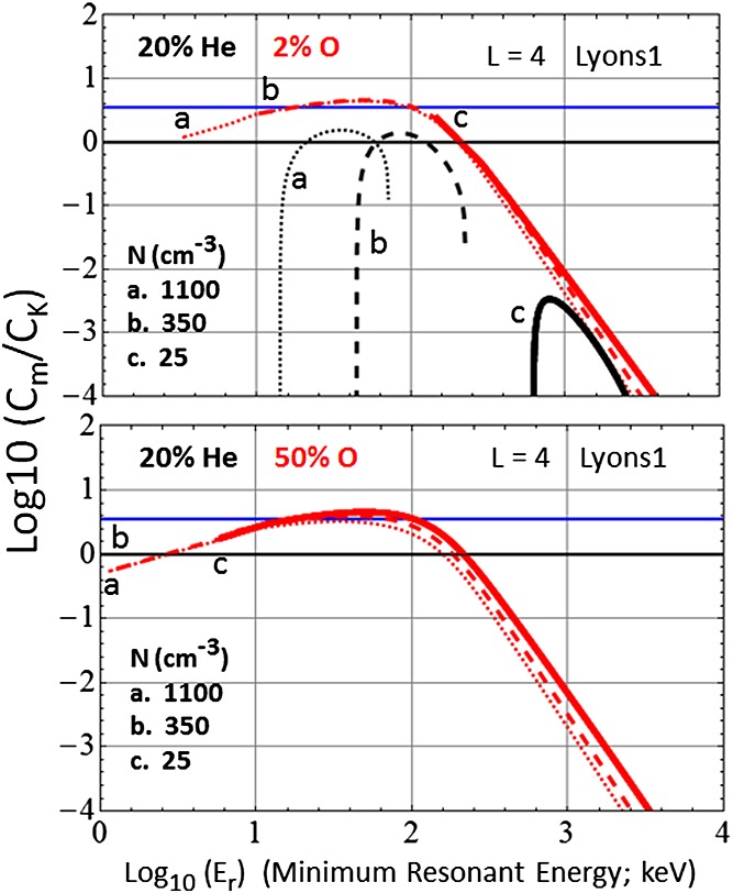
Differential Kennel-Petschek analyses (the C_m/C_K profiles specified by equation (4)) of energetic ion spectra sampled in the ring current regions of Earth's inner magnetosphere. It shows the comparison of the KP results for an L = 4 spectrum (the first L = 4 spectrum in Table1) when the O⁺ contribution is (top) 2% and (bottom) 50%. The red curves are the contributions from the LT(O⁺) mode, and the black curves are contributions from the LT(He⁺) mode. The LT(H⁺) mode does not contribute substantially for the parameters used for these plots, and the LT(He⁺) contribution disappears in the lower plot when the O⁺ contributions are increased. For each panel, three different densities are used and are represented with dotted, dashed, and solid lines and with labels “a,” “b,” and “c.” The lower two total plasma densities used for each panel is based on the Sheeley et al. [2001] for the given L value, and the highest is based on the densities that arise with a fully formed plasmasphere [Chappell, 1972].

What we see in Figure5 (top) is that the chosen spectrum is more than a factor of 4 higher than the classical Kennel-Petschek limit over a range of resonant energies. This result occurs relatively consistently for a broad range of intense proton spectra observed in Earth's inner magnetosphere [Mauk, 2013]. Based on that observation, the blue horizontal line in Figure5 is viewed as representing an empirically derived Kennel-Petschek limit. That limit can be achieved by modest alterations of the standard parameters. There are three key parameters in the simple theory: D (the distance along the magnetic field where the wave growth remains positive and high), R (the wave reflective or feedback coefficient), and S (the assumed anisotropy parameter). The “classical” parameters are: D = L, R = 0.05, and S = 1/6 (the S parameter is somewhat L dependent). The blue horizontal line in the panels of Figure5 represents the relative level that would be achieved if we were to alter the parameters to the following: D = L/2, R = 0.005, and S = 1/6. Alternatively, one could choose to modify S to a smaller value, given the extremely flat pitch angle distributions reported by Williams and Lyons [1974a]; a numerical characterization is very difficult from the highly compressed plots provided. None of the “new” parameter possibilities (R, D, and S) for achieving quantitative concurrence with the KP expectations are unreasonable, but it is acknowledged that the need for manipulating the model parameters weakens arguments in favor of the efficacy of the KP limit for ions. Other details of the analyses in Figure5 and in Mauk [2013], however, argue more in favor of a role for the KP limit. For example, the spectral shapes for energies less than 100 keV are relatively flat for the most intense spectra, with low spectral index values (γ1; see Table1) similar to what is observed for the electrons. The results in Figure5 and other results from Mauk [2013] are further summarized in Table1. In that table, the peaks of the C_m/C_K values observed from the KP analysis are shown in the column labeled “CRM,” which is short for C-Ratio Maximum. The minimum resonant energy where that peak value was observed is provided in the column labeled “ErM.”

Mauk [2013] concluded the analysis summarized in Figure5 by saying that: “—the evidence discussed here provides indications that an energetic ion, differential KP limit is active in helping to control the maximum intensities of ring current ion intensities within Earth's inner magnetosphere, but the evidence is not definitive.” In the present paper we seek additional evidence by considering the ion spectra sampled at other planets throughout the solar system.

In the section that follows, we will be addressing the ion spectra of the outer planets Jupiter, Saturn, Uranus, and Neptune. Much background information was provided about these planetary magnetospheres in the early companion to the present work [Mauk and Fox, 2010]. Here we choose not to repeat that information and instead refer to the reader to that earlier work.

6. Outer Planet Ions

Five spectra from Jupiter are displayed in Figure1. Heavy ions, in the form of Sⁿ⁺ and Oⁿ⁺ are important constituents of Jupiter's magnetosphere, with Sⁿ⁺ dominating over Oⁿ⁺ for all of the energetic ion moments [Mauk et al., 2004]. Hence, we have chosen to display H⁺and Sⁿ⁺ spectra from the Galileo mission that are most intense at 100 keV and at 1 MeV (hence, four spectra). Figure1 also shows one Jupiter spectrum from the Voyager epoch because Jupiter has proven to be a dynamic place even though the major source of energy for magnetospheric processes in Jupiter's inner to middle magnetosphere is thought to be planetary rotation. Figure6 shows a comparison between a ring current moment sampled during the Voyager epoch of 1979 and several samples of that same moment during the Galileo epoch (1995 and 1999). The moment displayed is the current collected by a solid state detector utilized by the Voyager instrument and modeled for both the Voyager and Galileo epochs based on the spectral inputs [Mauk et al., 2004]. That moment is roughly proportional to energy flux (but somewhat modified according to some detector characteristics). What was found, and discussed by Mauk et al. [2004] is that the ring current population during the Voyager epoch was much inflated as compared to that observed during the Galileo epoch. The suggested reason for the variation, supported by other unrelated observations, was that the volcanic action of the moon Io emitted more copious amounts of neutral gas during the Galileo epoch than it did during the Voyager epoch. Such gases strongly degrade the energetic ion populations by charge exchange in the regions close to Io. The Voyager spectrum displayed in Figure1 was measured by a single, magnetic-field-shielded solid state detector which was not able, in design, to discriminate between heavy ions and light ions. However, detailed analyses by Mauk et al. [1996] demonstrated that the detector current shown in Figure6 could only be reproduced under the assumption that the measured ions are mostly heavy (Oⁿ⁺ or Sⁿ⁺).

Figure 6.

Jupiter radial profile of a hot plasma moment that illustrates that the Jupiter ring current populations measured by the Voyager 1 spacecraft in 1979 (the red and brown symbols and lines) were more intense than were the similar ring current populations measured by Galileo in 1995 (the green symbols and lines) and in 1999 (the blue symbols and lines). The labels JOI, C23, E19, E26, E4, and E6 refer to specific orbits of the Galileo spacecraft. Labels like “95-341” refer to the year (1995 for this example) and the day of year (341 for this example). The moment that is plotted is the detector current measured by a solid state detector on Voyager and as modeled for Voyager and Galileo based on the measured spectral inputs. The detector current is roughly proportional to ion energy flux. The plot is from Mauk et al. [2004] and further details are provided in that paper.

Figure7 (bottom) shows the Kennel-Petschek analyses for the five Jupiter spectra shown in Figure1 (Figure7 (top) is a replot of the Jupiter spectra from Figure1). It would appear from these analyses that Jupiter's energetic ion populations are constrained by the classical Kennel-Petschek limit. Assuming that the Kennel-Petschek limit is playing the role ascribed to it here, the reason why Jupiter's ion populations would be constrained by the classical limit whereas Earth's ion populations are constrained by a somewhat higher level (factor of ∽3) is not known. However, these systems are very different and it would not be a surprise if one or more of the fundamental parameters (D, R, and S) were also different. It is of interest that the C_m/C_K profiles from three out of four of the spectra obtained from the Galileo mission reach up to “contact” the C_m/C_K = 1 line at various ranges of energy. It is only the Voyager spectrum, observed during the period of the inflated ring current epoch, that has a C_m/C_K profile that lies flat against the C_m/C_K = 1 line over an extended range of energies. That is also the Jupiter spectrum in Figure1 that is the flattest for energies below a break point near ∽2 MeV.

Figure 7.

(top) A replotting of the Jupiter energetic ion spectra shown in Figure1. (bottom) The Kennel-Petschek analysis of the Jupiter spectra, comprising the C_m/C_K profiles derived using equation (4).

The KP analyses for the Saturn spectra shown in Figure1 and replotted in Figure8 (top) are presented in Figure8 (bottom). Saturn is clearly a very different place in that its spectra do not challenge the KP limit at any energy. This result for ions is consistent with the results for electrons. As with the electrons, we assume that the copious presence of neutral gas and dust degrades the ion spectra faster than the ions can be accelerated to the highest levels [Paranicas et al., 2008].

Figure 8.

(top) Saturn ion spectra replotted from Figure1. (bottom) The Kennel-Petschek analysis of the three Saturn ion spectra, comprising the C_m/C_K profiles derived using equation (4).

The results of our KP analyses for Uranus and Neptune are shown in Figure9, as a part of a five planet summary of the results of this paper. The most intense ion spectra from Uranus and Neptune join Saturn in being far below their respective KP limits. Figure9 makes it doubly clear how special both Earth and Jupiter are with respect to the robustness of the acceleration processes that are happening. The question naturally arises as to whether simple modifications of the R, D, and/or S parameters might bring Uranus and Neptune (and Saturn) into line with Earth and Jupiter as magnetospheres with KP-limited ion spectra, in the same way that the nominal factor of 3 difference between Earth and Jupiter's has been reconciled. That question is discussed in the section 8.

Figure 9.

(top) A five-planet comparison of sample intense ion spectra from Earth (E), Jupiter (J), Saturn (S), Uranus (U), and Nepture (N). The Earth spectrum is the second L = 4 spectrum in Table1 (different than the one used for Figure5). The numbers following the planet designation is the approximate L value where the spectrum was sampled. The symbols H, O, and S refer to hydrogen, oxygen, and sulfur ions. (bottom) The Kennel-Petschek analyses of those same five spectra comprising the C_m/C_K profiles derived using equation (4).

7. Other Limiting Factors

The Kennel-Petschek limit is a highly nonlinear limit representing a relatively sharply defined upper threshold or demarcation. For magnetospheres that do not challenge the KP limit, there is no reason that a magnetospheric population must be limited by such a sharply defined limit. For such magnetospheres it is a reasonable assumption that there exists a quasi-linear balance between source and loss processes. At Saturn, for example, ion populations that are energized in the middle to outer magnetosphere are transported (by diffusion arising from multiplicities of small-scale injections) into the increasingly dense neutral gas and dust populations generated by the plumes of Saturn's moon Enceladus [Dougherty et al., 2009]. If the transport and energization rates increase, the populations are transported more deeply into the gas and dust populations before they are overcome by charge exchange and scattering losses [Paranicas et al., 2008]. Other magnetospheres may establish a quasi-linear source versus loss balance using the very same wave- particle losses considered here for the Kennel-Petschek limit. As intensities increase the wave growth, the corresponding wave intensities increase, causing increasing proportions of scattered losses. The difference there would be that the threshold would not have been crossed, whereby the feedback of wave energies would lead to runaway growth, giving rise to a sharp threshold.

It is worth considering whether there might be other threshold-inducing mechanisms. One possibility is that particle pressures might increase to the extent that the magnetic field cannot mechanically contain the populations. Table1 shows two additional columns to address this point. “BD” is the dipole magnetic field strength at the position where the spectrum was measured (as distinct from the locally measured magnetic field strength) and “betaD” is the ratio of the integrated particle pressure (for the particular spectrum in question) normalized by the dipole magnetic field pressure. We have chosen to parameterize with the dipole field because the local measured magnetic field strength depends much on the configuration of electric currents over large-scale regions. This approach is commensurate with some characterizations of laboratory plasmas where the “beta” parameter is not the local particle pressure normalized by the local magnetic field strength, but rather the internal particle pressure normalized by the external magnetic field that is confining the plasma. Note that for the configuration of a single plasma-populated flux tube within an otherwise vacuum field, a “betaD” of 0.5 would correspond roughly to a traditional local plasma beta parameter equal to 1, since inside the flux tube plasma and magnetic field pressures would be roughly equal. Clearly if “betaD” approaches the value of 1, as it does for the Earth L = 5 spectrum in Table1, it is reasonable to assume that the system might struggle to contain such a population. Whether or not the system would struggle to contain lower values of betaD is a question that we are unable to answer here. But it is of substantial interest that for the two magnetospheres that seem to challenge the KP limit, Earth and Jupiter, the betaD values for the most intense spectra are very different for the two planets; Earth's are relatively high whereas Jupiter's are all very low. It is clear that the KP limit comes closest to ordering the vast differences between the Jupiter and Earth spectra than do pressure balance considerations.

8. Summary and Discussion

We have compared the most intense energetic ion spectra that comprise the magnetospheric ring current populations in all five of the strongly magnetized planets of the solar system, specifically at Earth, Jupiter, Saturn, Uranus, and Neptune. The chosen spectra are most intense at 100 keV, 1 MeV, or both. Acknowledging the limitations of comparing spectra obtained from orbital missions (Earth, Jupiter, and Saturn) with those measured during single flybys (Uranus and Neptune), we note that the spectra are diverse in intensity at selected energies by as much a 4 orders of magnitude, substantially greater than the mere 2 orders of magnitude diversity of “most intense” electron spectra within these very same systems. We find for energies <0.5 MeV that Earth's energetic ion spectra are by far more intense than are the spectra of any other planet. For energies >1 MeV, Jupiter has by far the most intense ion spectra.

We have tested the degree to which the spectral diversity might be ordered by an updated version of the classical Kennel-Petschek limit, taking into account the diversity of ion species within these various systems. We find that, given some flexibility in specifying the parameters that go into the classic theory, all of these most intense ion spectra have intensities that are comparable to, below, or far below the Kennel-Petschek limit; and that therefore the ion Kennel-Petschek limit does represent a true threshold for the intensities of energetic ions within planetary magnetospheres. However, only the ring current populations of Earth and Jupiter have acceleration processes sufficiently robust to clearly challenge the Kennel-Petsheck limit. The observed “most intense” spectra of Saturn, Uranus, and Neptune reside far below this limit at all energies. Earth and Jupiter spectra that challenge the KP limit over extended ranges of resonant energies also have the characteristic flat energy distributions (low spectral indices) within the region of minimum resonant energies where the limits are challenged. These observations suggest that these spectra are sculpted by the KP process. The fact that only Earth and Jupiter have reports in the literature of definitive measurements of EMIC waves thought to be generated by hot anisotropic ions (and not by the ion pickup process), as discussed at the end of section 3, is consistent with the findings reported here that only at Earth and Jupiter do the most intense ion spectra seem to challenge the KP limit.

The question arises as to whether the C_m/C_K profiles calculated for Neptune, Uranus, or Saturn might be raised and brought into line with those of Earth and Jupiter by modifying one or more of the relevant parameters: R, D, or S; just as was done for Earth to reconcile the roughly factor of 3–4 (average) discrepancy when the Earth C_m/C_K profile peaks were consistently found to be somewhat higher than expected. The factors that must be made up are ∽11 for Saturn, ∽30 for Uranus, and ∽160 for Neptune (Figure9). For the parameter D it is hard to imagine that it can be much greater than L given the great variation in plasma and magnetic field parameters along the field lines; one could possibly stretch credibility by increasing D by a factor of 2, thereby increasing C_m/C_K by a corresponding factor of 2. It is also unlikely that the R factor can help us very much since it enters into the C_m/C_K logarithmically. If we modify R to its theoretical limit, that is, change it from 0.05 to 1, representing the highly unrealistic 100% reflective feedback into the system, C_m/C_K can be increased by only ln [1/0.05] = a factor of 3, a highly unlikely additional factor that even still does not solve the problem. It might be reasonable to allow an overall combined factor of 2 to be achieved by some manipulations of the R and D parameters. That leaves us with the S factor. While we can certainly contemplate modest increases in the S parameter (e.g., factor of 2), large increases would violate the fundamental premise of the Kennel-Petschek process. It is assumed with that process that once the EMIC wave turbulence becomes strong in association with reflective feedback, the pitch angle distributions are strongly flattened such that the scattering losses approach the so-called strong diffusion limit. And since such strong flattening is certainly observed at Earth [Williams and Lyons, 1974a], there is no reason why such flattening would not also accompany strong EMIC wave turbulence at other planets. For completeness we show in Figure10 that a substantial violation of our assumption about the flattening of the pitch angle distributions can indeed move the C_m/C_K profiles for Saturn, Uranus, and Neptune substantially closer to the limit line. Here a rather typical quiet time or storm recovery phase pitch angle anisotropy of S = 1 is assumed [e.g., Williams and Lyons, 1974b; Lui et al., 1990; Chen et al., 1998]. However, again, Figure10 violates the fundamental premise of the Kennel-Petschek limit and therefore cannot be used to alter our general conclusions about Saturn, Neptune or Uranus. In the paragraphs that follow, we address the individual issues raised with the results at these three planets.

Figure 10.

A recalculation of the C_m/C_K profiles shown in Figure9 for Saturn, Uranus, and Neptune but using a much larger anisotropy factor S = 1 (rather than 0.17 or 1/6). However, this figure is included for completeness only; as described in the main text, the assumption of a large anisotropy factor for a spectrum that is challenging the Kennel-Petschek limit is contrary to the fundamental premise of that Kennel-Petschek idea.

Although Saturn is a highly active magnetosphere [Mitchell et al., 2009], the results for Saturn are not surprising given the dense clouds of neutral gas and dust which engender very fast loss rates for energetic ions via the charge exchange process [Paranicas et al., 2008].

Uranus is an interesting case because (a) its electron populations show evidence of very robust acceleration processes that challenge the electron KP limit over an extended range of energies (Figure4), (b) observations suggest that Uranus' magnetosphere was very dynamic during the Voyager 2 encounter [Mauk et al., 1987, 1995; Sittler et al., 1987; Belcher et al., 1991], probably as a result of solar wind interactions given the Sun-Uranus alignment of the Uranian spin axis [Selesnick and McNutt, 1987], and (c) the whistler mode emissions, thought to be an important agent of electron acceleration were particularly intense [Kurth and Gurnett, 1991]. Thus, it is fair to say that the Uranian magnetosphere was highly active during the Voyager 2 flyby, but nonetheless the level of ion acceleration appears not to have been commensurate with the level of electron acceleration.

Neptune's magnetosphere was quiet during the Voyager 2 encounter, and there is the question as to whether it is ever particularly active. Neptune's interaction with the solar wind is expected to be weak, and there is no strong internal source of plasma, like that at Saturn and Jupiter, that can be energized by the rapid rotation of the planet. No residual signatures of dynamic injections were evident in the energetic particle data, the radial profiles of energetic particles were the most symmetric observed within the magnetospheres of the outer planets, and the energetic ion spectra quantitatively formed nearly perfect Maxwellians or Kappa distributions, a condition that is actually quite rare within planetary magnetospheres [Mauk et al., 1995]. It is a fair guess, although not certain, that the lack of robust ion (and electron) acceleration at Neptune is a general characteristic of that magnetosphere.

Regarding the use of the differential Kennel-Petschek as a standard for comparing spectra and acceleration processes at different planets, again, as acknowledged in Mauk [2013], it is well understood that the generation and propagation of EMIC waves in planetary magnetospheres can be far more complicated than the simple model represented here [e.g., Omidi et al., 2013; Silin et al., 2011]. The question is can a simplified recipe be found that provides an approximate standard for comparing different space environments and conditions? Such a simple recipe seems to work fairly well for the electrons (Figure4) despite the well-known complexities of whistler-electron interactions. The proof resides in the extent to which we can obtain consistent results over a broad range of events and environments.

The fact that Jupiter's energetic ion spectra appear to be well ordered by the Kennel-Petschek limit adds considerable new evidence in favor of the efficacy of the Kennel-Petschek limit as an ordering mechanism for energetic ions. However, the variations of the results between Earth and Jupiter (the two planets needing different KP parameters) make the evidence somewhat less convincing than that for the electron results. Again, the most definitive evidence may in the future come from detailed studies needed using the comprehensively instrumented Van Allen Storm Probes Mission launched 30 August 2012, now that instrument responses are well understood and once a diversity of storms is encountered.

To date the geomagnetic storms occurring since the launch of the Van Allen Probes mission and the full commissioning of the instruments have been modest; the storm of 17 March 2013 was the most intense at Dst ∽ −130 nT, with “betaD” values roughly 1/3 of the higher values shown in Table1 when compared at each value of L (using pressures provided by Gkioulidou et al. [2014]). Questions that can be addressed now are as follows: to what extent do modest storms challenge the Kennel-Petschek limit, or is this limit only challenged during the strongest storms? How does the distribution of EMIC wave modes (among LT(H⁺), LT(He⁺), and LT(O⁺)) change with activity level, and does the LT(O⁺) mode become more prominent with respect to the other modes during the strongest or most active storms? Is any change in that distribution correlated with the flattening of the energetic ion pitch angle distributions during modest and strong storms?

APPENDIX

Appendix A

The dispersion relationships for the propagation of electromagnetic ion cyclotron (EMIC) waves plotted in Figures2 and 3, and used in equations (5)–(7) for determining V_φ are derived directly from equations in Stix [1992]. The source equations are reproduced here for convenience. The vector and scalar of the so-called index of refraction (n and n) are defined as follows:

A1

A2

where k is the wave vector (magnitude 2π/λ where λ is the wavelength), c is the speed of light, ω is the wave frequency (2π/T where T is the wave period), and V_ϕ is the wave phase speed. Most critical for the present purposes is the determination of the wave phase speed V_ϕ. That function is determined by solving that following quadratic (in n²) equation:

A3

where:

A4

A5

A6

where θ is the angle of the k vector with respect to the background magnetic field B₀, and where

A7

A8

A9

A10

A11

A12

and where n_i is the density of species “i,” q_i is the charge of species i, and m_i is the mass of species i. Note that electrons are one of the species that must be included, and the summations are over electrons plus all charged ion species. The final solutions for n² (and then for V_ϕ) using a multispecies plasma, with up to six ion species, as considered in the present work, is exceedingly messy. Modern technology in the form of symbolic operation routines like Mathematica® aids greatly in the manipulation of these solutions.

The wave ellipticity equation used to create Figure2 (bottom) and to determine the ellipticity-dependent coloration of the lines in Figures3 and 2 (top) is

A13

A14

Key Points

• The Kennel-Petschek (KP) limit standardizes energetic ion spectra comparisons

• Only Earth and Jupiter spectra are limited-sculpted by the differential KP limit

• The efficacy of the KP limit for ions needs to be tested by the Van Allen Probes

References

- Barbosa DD. Theory and observations of electromagnetic ion cyclotron waves in Saturn's inner magnetosphere. J. Geophys. Res. 1993;98(A6):9345–9350. , doi: 10.1029/93JA00476. [Google Scholar]
- Belcher JW. The low energy plasma in the Jovian magnetosphere. In: Dessler AJ, editor. The Physics of the Jovian Magnetosphere. Cambridge, and New York: Cambridge Univ. Press; 1983. p. 68. Cambridge Planet. Sci. Ser edited by. [Google Scholar]
- Belcher JW, McNutt RL, Jr, Richardson JD, Selesnick RS, Sittler EC., Jr Bagenal F. The plasma environment of Uranus. In: Bergstralh JT, editor; Uranus. Tucson: Univ. of Ariz. Press; 1991. p. 780. , edited by et al., and. [Google Scholar]
- Boyd TJM. Sanderson JJ. Plasma Dynamics. New York: Barnes and Noble, Inc; 1969. [Google Scholar]
- Chappell CR. Recent satellite measurements of the morphology and dynamics of the plasmasphere. Rev. Geophys. 1972;10(4):951–979. , doi: 10.1029/RG010i004p00951. [Google Scholar]
- Chen L, Thorne RM. Bortnik J. The controlling effect of ion temperature on EMIC wave excitation and scattering. Geophys. Res. Lett. 2011;38 and, L16109, doi: 10.1029/2011GL048653. [Google Scholar]
- Chen MW, Roeder JL, Fennell JF, Lyons LR. Schulz M. Simulations of ring current proton pitch angle distributions. J. Geophys. Res. 1998;103(A1):165–178. and, doi: 10.1029/97JA02633. [Google Scholar]
- Daglis IA, Thorne RM, Baumjohan W. Orsini S. The terrestrial ring current: Origin, formation, and decay. Rev. Geophys. 1999;37(4):407–438. and, doi: 10.1029/1999RG900009. [Google Scholar]
- Davidson GT, Filbert PC, Nightingale RW, Imhof WL, Reagan JB. Whipple EC. Observations of intense trapped electron fluxes at synchronous altitudes. J. Geophys. Res. 1988;93(A1):77–95. and, doi: 10.1029/JA093iA01p00077. [Google Scholar]
- Dougherty MK, Esposito LW. Krimigis SM. Saturn from Cassini-Huygens. Dordrecht, and New York: Springer; 2009. [Google Scholar]
- Erlandson RE. Ukhorskiy AJ. Observations of electromagnetic ion cyclotron waves during geomagnetic storms: Wave occurrence and pitch angle scattering. J. Geophys. Res. 2001;106(A3):3883–3895. and, doi: 10.1029/2000JA000083. [Google Scholar]
- Gkioulidou M, Ukhorskiy AY, Mitchell DG, Sotirelis T, Mauk BH. Lanzerotti LJ. The role of small-scale ion injections in the buildup of Earth's ring current pressure: Van Allen Probes observations of the 17 March 2013 storm. J. Geophys. Res. Space Physics. 2014;119:7327–7342. and, doi: 10.1002/2014JA020096. [Google Scholar]
- Horwitz JL, Brace LH, Comfort RH. Chappell CR. Dual-spacecraft measurements of plasmasphere-ionosphere coupling. J. Geophys. Res. 1986;91(A10):11,203–11,216. and, doi: 10.1029/JA091iA10p11203. [Google Scholar]
- Keika K, Nose M, Brandt P, Ohtani S, Mitchell DG. Roelof EC. J. Geophys. Res. 2006;111 Contribution of charge exchange loss to the storm time ring current decay: IMAGE/HENA observations and, A11S12, doi: 10.1029/2006JA011789. [Google Scholar]
- Kennel CF. Petschek HE. Limit on stably trapped particle fluxes. J. Geophys. Res. 1966;71(1):1–28. and, doi: 10.1029/JZ071i001p00001. [Google Scholar]
- Krall NA. Trivelpiece AW. Principles of Plasma Physics. New York: McGraw-Hill; 1973. [Google Scholar]
- Krimigis SM, Gloeclker G, McEntire RW, Potemra TA, Scarf FL. Shelley EG. The magnetic storm of September 4, 1984, a synthesis of ring current spectra and energy densities measured with AMPTE/CCE. Geophys. Res. Lett. 1985;12(5):329–332. and, doi: 10.1029/GL012i005p00329. [Google Scholar]
- Krimigis SM, Armstrong TP, Axford WI, Cheng AF, Gleoeckler G, Hamilton DC, Keath EP, Lanzerotti LJ. Mauk BH. The magnetosphere of Uranus: Hot plasma and radiation environment. Science. 1986;233:97. doi: 10.1126/science.233.4759.97. and, doi: 10.1126/science.233.4759.97. [DOI] [PubMed] [Google Scholar]
- Krimigis SM. Magnetosphere Imaging Instrument (MIMI) on the Cassini Mission to Saturn/Titan. Space Sci. Rev. 2004;114:233–329. et al. (, doi: 10.1007/s11214-004-1410-8. [Google Scholar]
- Kurth WS. Gurnett DA. Plasma waves in planetary magnetospheres. J. Geophys. Res. 1991;96(Supplement):18,977–18,991. and, doi: 10.1029/91JA01819. [Google Scholar]
- Leisner JS, Russell CT, Wei HY. Dougherty MK. Probing Saturn's ion cyclotron waves on high-inclination orbits: Lessons for wave generation. J. Geophys. Res. 2011;116 and, A09235, doi: 10.1029/2011JA016555. [Google Scholar]
- Lin N, Kellogg PJ, MacDowall RJ, Mei Y, Cornilleau-Wehrlin N, Canu P, de Villedary C, Rezeau L, Balogh A. Forsyth RJ. ULF waves in the Io torus: Ulysses observations. J. Geophys. Res. 1993;98(A12):21,151–21,162. and, doi: 10.1029/93JA02593. [Google Scholar]
- Lui ATY, McEntire RW, Sibeck DG. Krimigis SM. Recent findings on angular distributions of dayside ring current energetic ions. J. Geophys. Res. 1990;95(A12):20,839–20,851. and, doi: 10.1029/JA095iA12p20839. [Google Scholar]
- Lyons LR. Williams DJ. A source for the geomagnetic storm main phase ring current. J. Geophys. Res. 1980;85(A2):523–530. and, doi: 10.1029/JA085iA02p00523. [Google Scholar]
- Mauk BH. Helium resonance and dispersion effects on geostationary Alfven/ion-cyclotron waves. J. Geophys. Res. 1982;87(A11):9107–9119. doi: 10.1029/JA087iA11p09107. [Google Scholar]
- Mauk BH. Frequency gap formation in electromagnetic cyclotron wave distributions. Geophys. Res. Lett. 1983;10:635–638. doi: 10.1029/GL010i008p00635. [Google Scholar]
- Mauk BH. Analysis of EMIC-wave-moderated flux limitation of measured energetic ion spectra in multispecies magnetospheric plasmas. Geophys. Res. Lett. 2013;40:3804–3808. doi: 10.1002/grl.50789. [Google Scholar]
- Mauk BH. Fox NJ. Electron radiation belts of the solar system. J. Geophys. Res. 2010;115 and, A12220, doi: 10.1029/2010JA015660. [Google Scholar]
- Mauk BH. McPherron RL. An experimental test of the electromagnetic ion cyclotron instability within the Earth's magnetosphere. Phys. Fluids. 1980;23(10):2111. [Google Scholar]
- Mauk BH, Krimigis SM, Keath EP, Cheng AF, Armstrong TP, Lanzerotti LJ, Gloeckler G. Hamilton DC. The hot plasma and radiation environment of the Uranian magnetosphere. J. Geophys. Res. 1987;92(A13):15,283–15,308. and, doi: 10.1029/JA092iA13p15283. [Google Scholar]
- Mauk BH, Krimigis SM, Cheng AF. Selesnick RS. Energetic particles and hot plasmas of Neptune. In: Cruikshank DP, editor; Neptune and Triton. Tucson: Univ. of Ariz. Press; 1995. p. 169. edited by, and. [Google Scholar]
- Mauk BH, Gary SA, Kane M, Keath EP, Krimigis SM. Armstrong TP. Hot plasma parameters of Jupiter's inner magnetosphere. J. Geophys. Res. 1996;101(A4):7685–7695. and, doi: 10.1029/96JA00006. [Google Scholar]
- Mauk BH, Mitchell DG, McEntire RW, Paranicas CP, Roelof EC, Williams DJ, Krimigis SM. Lagg A. Energetic ion characteristics and neutral gas interactions in Jupiter's magnetosphere. J. Geophys. Res. 2004;109 and, A09S12, doi: 10.1029/2003JA010270. [Google Scholar]
- Mauk BH. Fundamental plasma processes in Saturn's magnetosphere. In: Dougherty MK, editor. Saturn from Cassini Huygens. Dordrecht, and New York: Springer; 2009. p. 281. edited by et al., et al. ( [Google Scholar]
- Min K, Lee J, Keika K. Li W. Global distribution of EMIC waves derived from THEMIS observations. J. Geophys. Res. 2012;117 and, A05219, doi: 10.1029/2012JA017515. [Google Scholar]
- Mitchell DG, Carbary JF, Cowley SWH, Hill TW. Zarka P. The dynamics of Saturn's magnetosphere. In: Krimigis SM, editor; Dougherty MK, Esposito LW, editors. Saturn From Cassini-Huygens. Dordrecht, and New York: Springer; 2009. p. 257. and, and,, edited by. [Google Scholar]
- Omidi N, Bortnik J, Thorne R. Chen L. Impact of cold O+ ions on the generation and evolution of EMIC waves. J. Geophys. Res. Space Physics. 2013;118:434–445. and, doi: 10.1029/2012JA018319. [Google Scholar]
- Paranicas C, Mitchell DG, Krimigis SM, Hamilton DC, Roussos E, Krupp N, Jones GH, Johnson RE, Cooper JF. Armstrongh TP. Sources and losses of energetic protons in Saturn's magnetosphere. Icarus. 2008;197:516–525. [Google Scholar]
- Richardson JD, Belcher JW, Szabo A. McNutt RL., Jr . The plasma environment of Neptune. In: Cruikshank DP, editor; Neptune and Triton. Tucson, Ariz: Univ. of Ariz. Press; 1995. p. 279. edited by, and. [Google Scholar]
- Roux A, Perraut S, Rauch JL, deVilledary C, Kremser G, Korth A. Young DT. Wave-particle interactions near ΩHe+ observed on board GEOS 1 and 2: 2. Generation of ion cyclotron waves and heating of He+ ions. J. Geophys. Res. 1982;87(A10):8174–8190. and, doi: 10.1029/JA087iA10p08174. [Google Scholar]
- Russell CT, Leisner JS, Arridge CS, Dougherty MK. Blanco-Cano X. Nature of magnetic fluctuations in Saturn's middle magnetosphere. J. Geophys. Res. 2006;111 and, A12205, doi: 10.1029/2006JA011921. [Google Scholar]
- Schulz M. Davidson GT. Limiting energy spectrum of a saturated radiation belt. J. Geophys. Res. 1988;93(A1):59–76. and, doi: 10.1029/JA093iA01p00059. [Google Scholar]
- Selesnick RS. McNutt RL., Jr Voyager 2 plasma ion observations in the magnetosphere of Uranus. J. Geophys. Res. 1987;92(A13):15,249–15,262. and, doi: 10.1029/JA092iA13p15249. [Google Scholar]
- Sergis N. Particle pressure, inertial force, and ring current density profiles in the magnetosphere of Saturn, based on Cassini measurements. Geophys. Res. Lett. 2010;37 et al. (, L02102, doi: 10.1029/2009GL041920. [Google Scholar]
- Sheeley BW, Moldwin MB, Rassoul HK. Anderson RR. An empirical plasmasphere and trough density model: CRRES observations. J. Geophys. Res. 2001;106(A11):25,631–25,641. and, doi: 10.1029/2000JA000286. [Google Scholar]
- Silin I, Mann IR, Sydora RD, Summers D. Mace RL. Warm plasma effects on electromagnetic ion cyclotron wave MeV electron interactions in the magnetosphere. J. Geophys. Res. 2011;116 and, A05215, doi: 10.1029/2010JA016398. [Google Scholar]
- Sittler EC, Jr, Ogilvie KW. Selesnick RS. Survey of electrons in the Uranian magnetospshere, Voyager 2 observations. J. Geophys. Res. 1987;92(A13):15,263–15,262. and, doi: 10.1029/JA092iA13p15263. [Google Scholar]
- Stix TH. Waves in Plasmas. Springer, New York; 1992. [Google Scholar]
- Summers D. Shi R. Limiting energy spectrum of an electron radiation belt. J. Geophys. Res. Space Physics. 2014;119:6313–6326. and, doi: 10.1002/2014JA020250. [Google Scholar]
- Summers D, Tang R. Thorne RM. Limit on stably trapped particle fluxes in planetary magnetospheres. J. Geophys. Res. 2009;114 and, A10210, doi: 10.1029/2009JA014428. [Google Scholar]
- Tang R. Summers D. Energetic electron fluxes at Saturn from Cassini observations. J. Geophys. Res. 2012;117 and, A06221, doi: 10.1029/2011JA017394. [Google Scholar]
- Thomsen MF, Reisenfeld DB, Delapp DM, Tokar RL, Young DT, Crary FJ, Sittler EC, McGraw MA. Williams JD. Survey of ion plasma parameters in Saturn's magnetosphere. J. Geophys. Res. 2010;115 and, A10220, doi: 10.1029/2010JA015267. [Google Scholar]
- Ukhorskiy AY, Shprits YY, Anderson BJ, Takahashi K. Thorne RM. Rapid scattering of radiation belt electrons by storm-time EMIC waves. Geophys. Res. Lett. 2010;37 and, L09101, doi: 10.1029/2010GL042906. [Google Scholar]
- Usanova ME, Mann IR, Bortnik J, Shao L. Angelopoulos V. THEMIS observations of electromagnetic ion cyclotron wave occurrence: Dependence on AE, SYMH, and solar wind dynamic pressure. J. Geophys. Res. 2012;117 and, A10218, doi: 10.1029/2012JA018049. [Google Scholar]
- Williams DJ. Lyons LR. Further aspects of the proton ring current interaction with the plasmapause: Main and recovery phases. J. Geophys. Res. 1974a;79(31):4791–4798. and, doi: 10.1029/JA079i031p04791. [Google Scholar]
- Williams DJ. Lyons LR. The proton ring current and its interaction with the plasmapause: Storm recovery phase. J. Geophys. Res. 1974b;79(28):4195–4207. and, doi: 10.1029/JA079i028p04195. [Google Scholar]