

Abstract
We present analytic expressions for ULF wave-derived radiation belt radial diffusion coefficients, as a function of L and Kp, which can easily be incorporated into global radiation belt transport models. The diffusion coefficients are derived from statistical representations of ULF wave power, electric field power mapped from ground magnetometer data, and compressional magnetic field power from in situ measurements. We show that the overall electric and magnetic diffusion coefficients are to a good approximation both independent of energy. We present example 1-D radial diffusion results from simulations driven by CRRES-observed time-dependent energy spectra at the outer boundary, under the action of radial diffusion driven by the new ULF wave radial diffusion coefficients and with empirical chorus wave loss terms (as a function of energy, Kp and L). There is excellent agreement between the differential flux produced by the 1-D, Kp-driven, radial diffusion model and CRRES observations of differential electron flux at 0.976 MeV—even though the model does not include the effects of local internal acceleration sources. Our results highlight not only the importance of correct specification of radial diffusion coefficients for developing accurate models but also show significant promise for belt specification based on relatively simple models driven by solar wind parameters such as solar wind speed or geomagnetic indices such as Kp.
Key Points
Analytic expressions for the radial diffusion coefficients are presented
The coefficients do not dependent on energy or wave m value
The electric field diffusion coefficient dominates over the magnetic
1. Introduction
The Earth's outer radiation belt consists of relativistic electrons trapped in the Earth's geomagnetic field. In situ observations have shown that the flux of these electrons is highly variable [Blake et al., 1992; Li et al., 1993; Baker et al., 1994; Horne et al., 2005]. There is currently no model which can simulate the behavior of the outer radiation belt during every storm. However, one critical component of any radiation belt model is ULF wave-driven radial diffusion [Fälthammar, 1965; Schulz and Lanzerotti, 1974; Fei et al., 2006]. Several different approaches have been used to derive the ULF wave radial diffusion coefficients.
Brautigam and Albert [2000] separated the ULF wave radial diffusion coefficients into electrostatic and electromagnetic components. An expression for the analytic diffusion coefficient,  as a function of Kp corresponding to the electrostatic wave fluctuations was obtained by assuming that the electric field wave spectrum can be modeled as a substorm convection electric field characterized by a rapid rise time and an exponential decay [Cornwall, 1968; see also Brautigam and Albert, 2000]. Brautigam and Albert [2000] also derived expressions for the electromagnetic diffusion coefficients,
  again as a function of Kp, based on in situ compressional magnetic field power spectral density (PSD) measurements and ground magnetometer magnetic field PSD measurements mapped to the equatorial plane, binned by Kp. The limitations of the approach used in Brautigam and Albert [2000] are that the expressions for the electromagnetic diffusion coefficients as a function of Kp are only based on a small number of ULF wave magnetic field PSD measurements: 18 days of ground magnetometer measurements at L = 4 and 1 month of in situ measurements at L = 6.6. It is unlikely this short time interval of measurements at only two L shells is sufficient to accurately characterize the average magnetic field PSD as a function of Kp and L shell, yet this was used to derive the analytic expressions for the electromagnetic diffusion coefficients in Brautigam and Albert [2000]. In addition, the method used to map the ground PSD values to the compressional magnetic field PSD values in space in the magnetic equatorial plane also assumes that the PSD values are azimuthally symmetric and correspond to symmetric perturbations of the Earth's main field with an effective dimensionless azimuthal wave number of m = 0 [Lanzerotti and Morgan, 1973]. In reality, the measured magnetic field PSD values may be composed of a spectrum of wave perturbation solutions rather than perturbations to the main field, each with a different azimuthal wave number, m, [see, e.g., Sarris et al., 2006; Tu et al., 2012]. Despite these limitations, the analytic expression for the electromagnetic diffusion equation presented in Brautigam and Albert [2000] is currently used in most radiation belt models, such as Versatile Electron Radiation Belt [Subbotin and Shprits, 2009], SALAMMBO [e.g., Beutier and Boscher, 1995; Varotsou et al., 2008], and Dynamic Radiation Environment Assimilation Model (DREAM) [Koller et al., 2007]. Additionally, inclusion of the electrostatic along with the electromagnetic diffusion coefficient from Brautigam and Albert [2000] in these models produces electron flux results on low L shell much greater than the measured electron flux, and an intense inner zone, which unphysically large losses would be required to remove [see, e.g., Kim et al., 2011; see also Ozeke et al., 2012b]. Consequently, due to the unphysical nature of the results, the Brautigam and Albert [2000] electrostatic diffusion coefficient is usually excluded from radial diffusion simulations of the radiation belts, with only the electromagnetic diffusion being active in the radial transport [cf. Shprits et al., 2005]. This suggests that the Brautigam and Albert [2000] radial diffusion coefficients might be in need of revision, and in this paper we extend the work of Ozeke et al. [2012a] and present analytic expressions for new diffusion coefficients which are derived on the basis of ULF wave observations.
Brizard and Chan [2001] showed that the ULF wave-driven radial diffusion coefficients can be separated into terms due to the azimuthal electric field and the compressional magnetic field of the waves [see also Fei et al., 2006]. This approach allows the diffusion coefficients to be obtained directly from measurements of the waves electric and magnetic field PSD values taking into account the azimuthal wave number, m, of the waves. In Brautigam et al. [2005], CRRES measurements of the electric field PSD values taken over a 9 month period where used to derive expressions for the electric field diffusion coefficients using the approach outlined in Brizard and Chan [2001] [see also Fei et al., 2006]. In order to determine these electric field diffusion coefficients, it was assumed that all of the ULF wave power resulted from m = 1 waves. This assumption is consistent with the typical results from ULF wave simulations [Elkington et al., 2012] using the Lyon-Fedder-Mobarry magnetohydrodynamic code [Lyon et al., 2004] which show that the m = 1 mode is usually dominant, with the spectra usually comprising low mode numbers less than 3.
In Ozeke et al. [2012a] expressions for electric field diffusion coefficients as functions of Kp or solar wind speed were derived based on over 15 years of ground magnetometer measurements at 7 different L shells. Expressions for the compressional magnetic field diffusion coefficient were also derived using 10 years of GOES magnetic field PSD measurements and the Active Magnetospheric Particle Tracer Explorers (AMPTE) magnetic field PSD measurements presented in Takahashi and Anderson [1992]. However, the diffusion coefficient expressions presented in Ozeke et al. [2012a] are rather complex and difficult to implement in radial diffusion model simulations, requiring the use of large lookup tables to determine the coefficients. The Ozeke et al. [2012a] approach also assumed that the measured ULF wave magnetic and electric fields resulted from waves with a single azimuthal wave number, m.
In this paper we derive a simple analytic expression for the electric field diffusion coefficients based on the same ground magnetometer measurements presented in Ozeke et al. [2012a] which can be easily and analytically incorporated into radial diffusion models. In addition, we also derive a simple analytic expression for the magnetic field diffusion coefficients based on the same GOES magnetic field PSD measurements used in Ozeke et al. [2012a] with the addition of magnetic field PSD measurements taken from the five Time History of Events and Macroscale Interactions during Substorms (THEMIS) spacecraft.
2. Radial Diffusion Coefficients
The radial diffusion equation expressed in terms of L shell is given by equation (1)
| 1 |
In equation (1) f represents the phase space density of the electrons, and it is assumed that the first and second adiabatic invariants, M and J, are conserved [see Schulz and Lanzerotti, 1974]. The diffusion coefficient and the electron lifetime are represented by DLL and τ, respectively.
The diffusion coefficient, DLL, is the sum of the diffusion coefficients due to the (assumed) uncorrelated azimuthal electric field and the compressional magnetic field perturbations,  and
and  , respectively [see Ozeke et al., 2012a]. In a dipole magnetic field, the symmetric radial diffusion coefficients under drift resonance (where the electron drift speed matches the phase speed) due to these electric and magnetic field perturbations
  and
and  can be expressed as follows:
| 2 |
| 3 |
| 4 |
[see Brizard and Chan, 2001; Fei et al., 2006]. Here the constants BE, RE, and q represent the equatorial magnetic field strength at the surface of the Earth, the Earth's radius, and the electron charge, respectively. The relativistic correction factor, γ, is given by
| 5 |
Here v is the total speed of the electron and c is the speed of light. Of course, v does not remain constant but increases and decreases as the electrons diffuse radially inward and outward, respectively. M represents the first adiabatic invariant which depends on the electron's mass, me, and the perpendicular momentum, p⊥; see equation (4).
In equations (2) and (3) the terms  and
and  represent the PSD of the electric and magnetic field perturbations with azimuthal wave number, m, at wave frequency, ω, which satisfy the drift resonance condition given by equation (6)
| 6 |
Here ωd represents the bounce-averaged angular drift frequency of the electron [see Southwood and Kivelson, 1982; Brizard and Chan, 2001]. Since ωd is a function of the electron's energy and L shell, this introduces energy and L shell dependence into the PSD terms  and
and  in equations (2) and (3).
3. Power Spectral Densities
3.1. Azimuthal Electric Field PSD Fits
In Ozeke et al. [2012a] the equatorial azimuthal electric field PSD values as a function of Kp are derived from ground D-component magnetometer measurements (allowing for assumed 90° polarization rotation through the ionosphere) taken at L shells from L = 2.55 to L = 7.94, using a similar mapping technique to that presented in Ozeke et al. [2009] (see that paper for more details of the analysis procedure and the stations used). In Ozeke et al. [2009, 2012a] the ground magnetic field, bg, was mapped to the ionospheric magnetic field bi, using the method outlined in Hughes and Southwood [1976], where
| 7 |
Here k is the horizontal wave number of wave at the ionosphere. In order to derive the expression in equation (7), it was assumed in Hughes and Southwood [1976] that k−1 < 100 km.
However, the ULF waves of interest here typically have k−1 > 100 km and the mapping relationship between the ground and ionospheric magnetic fields presented in Hughes and Southwood [1976] shown in equation (7) is not appropriate for these waves. In this paper we use the method outlined in Glassmeier [1984], where k−1 > 100 km which increases the ground to ionospheric magnetic field mapping by a factor of 2, giving
| 8 |
A much more detailed approach for determining the relationship between the ground and ionospheric magnetic fields including the effects of an inductive ionosphere is also given in Yoshikawa and Itonaga [2000]. However, below frequencies of 10 mHz and k−1 > 100 km the results given in Yoshikawa and Itonaga [2000] are consistent with equation (8). This doubling of the ionospheric magnetic field bi mapped from the ground magnetic field bg causes the equatorial electric field PSD to be increased by a factor of 4 from the values in Ozeke et al. [2012a].
The new mapped equatorial azimuthal electric field PSD values derived from the database of ground D-component median PSD values as a function of Kp at each of the seven magnetometer stations used in Ozeke et al. [2012a] are illustrated by the circles in Figure 1. The dashed lines in Figure 1 represent simple analytic fits to the median azimuthal electric field PSD values as a function of Kp and L shell given by equation (9). The fits were produced by first calculating the mean value of the PSD at each of the L shell and Kp values shown in Figure 1. Next, the log10 of these mean PSD values was determined, and finally, using the method of least squares, these values were fit to linear functions of Kp and L shell.
Figure 1.
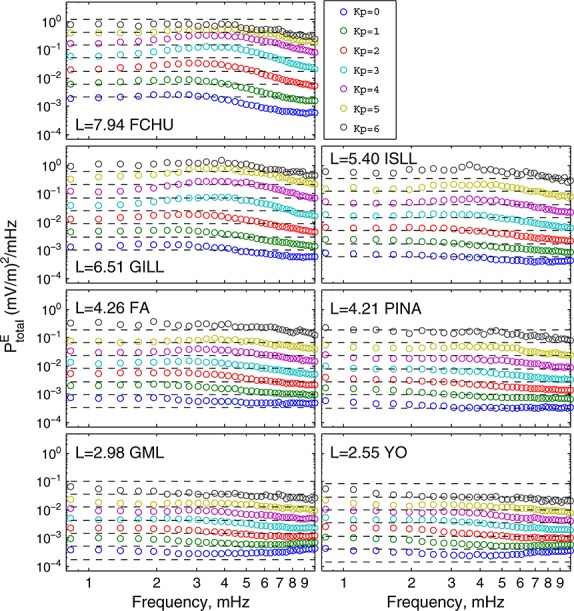
Azimuthal electric field PSD values derived from ground-based magnetometer measurements of the D-component magnetic field PSD at L = 7.94, 6.51, 5.40, 4.26, 4.21, 2.98, and 2.55. The dashed lines represent constant fits to these PSD values given by equation (9).
The simple fit in equation (9), although purely empirical in nature, is seen to provide a good representation of the electric field power across all Kp values and at all station L values, particularly those in the outer radiation belt region, from around L = 4 to L = 6.5. Hence, equation (9) provides an excellent analytic basis for including median ULF wave electric field power into radial diffusion coefficients. The mapped ULF wave electric field power is assumed in this fit to be independent of frequency (and hence electron energy under the action of drift resonant diffusion with fixed m) which is an especially good approximation for frequencies below around 6–7 mHz, and especially on L shells which span the outer radiation belt.
| 9 |
Here  represents the sum of electric field wave power in all azimuthal wave number components and is in units of (mV/m)2/mHz.
3.2. Compressional Magnetic Field PSD Fits
In Ozeke et al. [2012a] GOES data were used at L = 6.6 for all Kp, and the L shell dependence of compressional ULF wave power at Kp = 2 observed by AMPTE and reported by Takahashi and Anderson [1992] was assumed to apply for all Kp. In order to improve the representation of the magnetic diffusion coefficients presented in Ozeke et al. [2012a], a statistical database of compressional magnetic field PSD values as a function of Kp was further derived from THEMIS satellite measurements. The GOES compressional magnetic field PSD database binned with Kp is the same as that used in Ozeke et al. [2012a], which is consistent with the GOES compressional magnetic field PSD values shown in Huang et al. [2010].
The THEMIS database was obtained by measuring the PSD using a fast Fourier transform applied to a 20 min Hanning window length of data and binning the PSD values with Kp. The PSD measurements were taken using each of the THEMIS A, B, C, D, and E spacecraft from 2007 to 2011, and the THEMIS Data Analysis Software was used to rotate the data into a field-aligned coordinate system so that the compressional magnetic field component PSD could be found. During the period of the 20 min window, the spacecraft passed through less than one L shell and the THEMIS magnetic field PSD results were hence determined at the median L shell during this 20 min window. These PSD values at the median L shells were then placed into bins of widths L = 7.5–6.5, L = 6.5–5.5, and L = 5.5–4.5 corresponding to L = 7, 6, and 5. Increasing the window length to 1 h did not significantly alter the resulting PSD values.
The THEMIS spacecraft are on elliptical orbits close to the magnetic equatorial plane having the greatest velocity on the lower L shells. The velocity of the spacecraft through the ULF waves introduces a Doppler effect which distorts the spacecraft-measured compressional magnetic field PSD on lower L shells; for this reason we limit our data to L shells from L = 7 to L = 5.
In Figure 2 the median PSD values binned with Kp from the GOES and THEMIS statistical databases are represented by the circles. Due to the low number of THEMIS PSD measurements where Kp was greater than 4, we only show the THEMIS median PSD values for bins 1 Kp wide for Kp = 4 and below. One Kp width bins for higher Kp values are not statistically reliable due to the smaller number of counts during between 2007 and 2011 (cf. the 15 years of ground magnetometer data which are included in the statistics shown in Figure 1). The dashed lines in Figure 2 represent analytic fits to the compressional magnetic field PSD values as expressed in equation (10).
Figure 2.
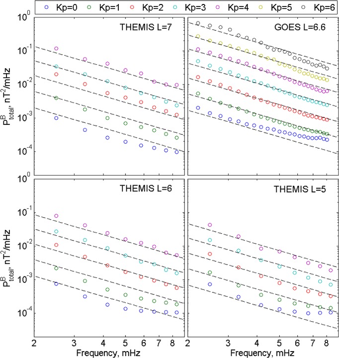
Median THEMIS and GOES compressional magnetic field PSD binned with Kp are represented by the circles. The analytic PSD fits from equation (10) are represented by the dashed lines.
The analytic fits to the GOES and THEMIS median compressional magnetic field PSD values as a function of Kp, L shell, and frequency; f are expressed as
| 10 |
Here  represents the compressional ULF wave power in all azimuthal wave number modes and in (10)
 is expressed in nT2/mHz, and where f is in megahertz. Here this fit assumes that the power spectra at any given L and Kp have a power law slope with an index of −2; Figure 2 shows this to be a good approximation across all L shells, and all Kp values, especially below around 6–7 mHz. Note also that (10) shows that the L dependence of power is to a good approximation the same for all Kp values—which was the assumption made in Ozeke et al. [2012a] where the observed Kp = 2 L dependence of compressional ULF wave power seen by AMPTE was further assumed for all Kp values.
4. Analytic Expressions for the Diffusion Coefficients
To derive analytic expressions for the diffusion coefficients, several assumptions about the measured electric and magnetic field PSD values have been made. First, we assume that all of the wave m values are positive (eastward propagating), since under symmetric drift resonance only positive wave m values contribute to resonant interactions and hence the diffusion coefficients; see equations (2) and (3). Second, we assume that the measured PSD, Ptotal, is the sum of the PSD's at each m value, Pm, so that
| 11 |
Finally, we also assume that each PSD at a specific m value, Pm, can be represented as some fraction, am, of the measured PSD, Ptotal, so that
| 12 |
The scale factors am are constants and are assumed to not depend on the wave frequency, f, or L shell. Of course, compressional modes such as waveguide modes may have turning points in L which do depend on frequency, and hence, this assumption is adopted for simplicity and tractability. Consequently, each specific Pm has the same L shell, frequency, and geomagnetic index (in this case Kp) dependence as Ptotal. Where diffusion coefficients are driven by solar wind parameters such as solar wind speed [cf., Rae et al., 2012] a similar approach could be adopted. Equations (11) and (12) imply that the sum of the scale factors must hence equal unity
| 13 |
| 14 |
4.1. Compressional Magnetic Field Diffusion Coefficient
The results presented in Figure 2 and equation (10) show that the compressional magnetic field PSD,  , can be approximated as a function of Kp and L multiplied by f− 2. However, Kp is not the only parameter which can be used to characterize ULF wave power. For example, Ozeke et al. [2012a] showed that the compressional magnetic field PSD,
  , may also be represented by functions of solar wind speed. To take into account the possibility that other parameters instead of Kp may also be used to characterize the wave power, we express
  more generally as
| 15 |
Here I can be a measure of the geomagnetic or solar (or solar wind) activity; in the case of Figures 1 and 2, I is represented by Kp, but this could also be solar wind speed [cf. Ozeke et al., 2012a] or some other parameter. For example, in Section 5 we showed that  in units of nT2/mHz can be expressed as a function of Kp, L, and frequency, f, in megahertz, as
| 16 |
An analytic expression for the magnetic diffusion coefficient can be derived by substituting equation (15) into equation (3) to give
| 17 |
The angular drift frequency, ωd, of 90° pitch angle radiation belt electrons in the equatorial plane of a dipole magnetic field is controlled by gradient drift and can be expressed as
| 18 |
Substituting equation (18) into equation (17) gives
| 19 |
Equation (19) illustrates that if the compressional magnetic field PSD at each wave m value varies  f− 2, as is shown to be a good approximation for the total PSD in Figure 2 up to ∼8 mHz, as well as in Takahashi and Anderson [1992] using AMPTE data, then the resulting magnetic diffusion coefficient produced by these ULF waves does not depend on the electrons M value (or energy). Instead, the diffusion coefficient only depends on the value of BTotal(L,I), which can be found directly from spacecraft measurements of the PSD. For example, based on our fits to the GOES and THEMIS compressional magnetic field PSDs expressed in equation (10), the magnetic diffusion coefficient in units of days−1 can be expressed analytically as
| 20 |
For frequencies above 8 mHz the assumption that the PSD at each wave m value varies ∝ f− 2 may no longer be valid, and at these high frequencies the magnetic diffusion coefficient may become a function of both wave m value and the electrons M value. However, in order for these >8 mHz waves to satisfy the drift resonance condition and contribute to the diffusion of the particles, the waves must have an m value ≳ 10 or the electrons must have energies ≳ 5 MeV.
In Figure 3 we show a comparison of our analytic magnetic diffusion coefficients (red line) with the magnetic diffusion coefficients derived directly from equation (3) using the GOES and THEMIS PSD measurements at L = 5, L = 6, L = 6.6, and L = 7 (squares and triangles) and using the compressional magnetic field PSD fits presented in Ozeke et al. [2012a] (dashed line). The diffusion coefficients represented by the green dashed lines (fits) and green squares (actual data) are derived assuming that all of the wave power is contained in m = 10 waves. Similarly, the diffusion coefficients represented by the red dashed lines (fits) and the red triangles (data) are derived assuming that all of the wave power is contained in m = 1 waves. The results in Figure 3 show that our analytic diffusion coefficients (red line) are in close agreement with both the diffusion coefficients derived from the THEMIS and GOES measurements at L = 5, L = 6, L = 6.6, and L = 7, as well as the magnetic field diffusion coefficients presented in Ozeke et al. [2012a]. The new element here is the use of THEMIS data across L and for all Kp, rather than the Ozeke et al. [2012a] approach to interpolate the observed Kp power dependence at Geostationary Earth Orbit (GEO) to other L shells, based on the assumption that the L dependence of the AMPTE compressional ULF wave power at Kp = 2 applied at all L and all Kp. As shown in (10), and in Figure 3, the Ozeke et al. [2012a] approach is in fact a rather a good approximation.
Figure 3.
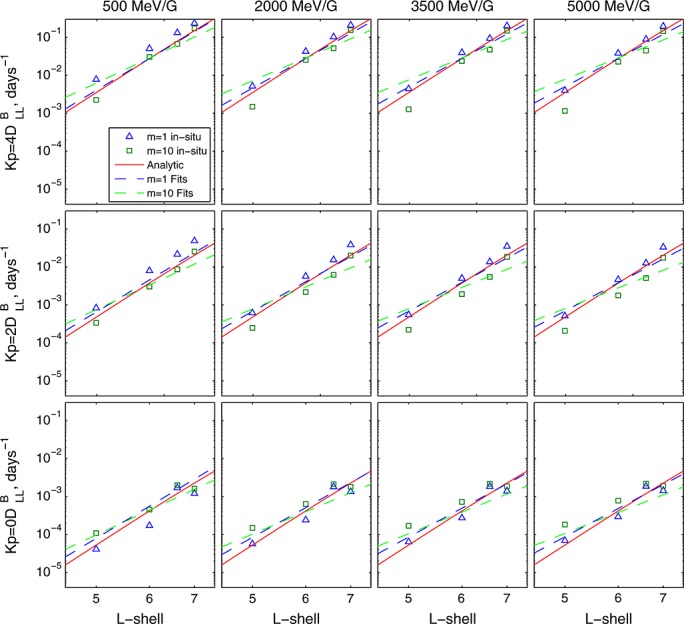
Magnetic diffusion coefficients: The symbols represent magnetic diffusion coefficients derived directly from the THEMIS and GOES spacecraft PSD measurements assuming wave m values of m = 10 (squares) and m = 1 (triangles). The dashed green (m = 10) and blue (m = 1) lines represent the magnetic diffusion coefficients derived from the tabulated PSD fits in Ozeke et al. [2012a]. The solid red line represents the magnetic diffusion coefficients given by equation (10).
4.2. Electric Field Diffusion Coefficient
If we assume that the azimuthal electric field PSD,  , in the equatorial plane of the magnetosphere is independent of frequency (seen to be a good approximation in Figure 1), depending only on the L shell and I, then we can write
| 21 |
For example, in section 3.1, equation (9) shows that  in units of (mV/m)2/mHz can be expressed as a function of Kp and L. Substituting equation (21) into equation (2) gives
| 22 |
If the electric field PSD  does not depend on frequency, then the resulting electric field diffusion coefficient produced by the ULF waves does not depend on the electrons M value. The electric field diffusion coefficients only depend on the (frequency independent) fits, ETotal(L,I), to the total PSD,
  which can be derived from spacecraft measurements of the PSD [e.g., Brautigam et al., 2005] or inferred from ground magnetometer observations [e.g., Rae et al., 2012; Ozeke et al., 2012a]. For example, based on our frequency independent fits to the electric field PSDs derived from the ground-based magnetometer measurements of the ULF waves illustrated in equation (9) and Figure 1, the electric diffusion coefficient in units of days−1 can be expressed analytically as
| 23 |
Here the scale factor of 2.156 × 10− 8 is required to give  in units of days−1, where
| 24 |
Figure 4 shows a comparison of our analytic electric diffusion coefficients (red line) with the exact values of the data-driven electric diffusion coefficients derived directly from equation (2) using the mapped ground-based magnetometer PSD measurements at L = 2.55, L = 2.98, L = 4.21, L = 4.26, L = 5.40, L = 6.51, and L = 7.94 (squares and triangles) and the fits to these mapped PSD values (dashed lines) from Ozeke et al. [2012a]. As discussed earlier, the mapping technique used here gives PSD values a factor of 4 larger than the mapped PSD values presented in Ozeke et al. [2012a]. Consequently, the electric field diffusion coefficients derived directly from our mapped PSD values shown by the square and triangle symbols in Figure 4 are a factor of 4 greater than the electric field diffusion coefficients values presented in Ozeke et al. [2012a]. Figures 3 and 4 also illustrate that the electric field diffusion coefficients are over a factor of 30 greater than the magnetic diffusion coefficients. This dominance of the electric over the magnetic diffusion coefficients was also shown in Ozeke et al. [2012a] and discussed further in Ozeke et al. [2012b].
Figure 4.
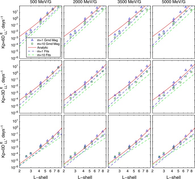
Electric diffusion coefficients: The symbols represent azimuthal electric field diffusion coefficients derived directly from the mapped ground PSD measurements (presented in Figure 1) and assuming wave m values of m = 10 (green squares) and m = 1 (blue triangles). The dashed green (m = 10) and blue (m = 1) lines represent the electric diffusion coefficients derived from the tabulated PSD fits in Ozeke et al. [2012a]. The red solid line represents the analytic electric field diffusion coefficients given by equation (9).
4.3. Diffusion Coefficient Comparison
In Figure 5 our analytic electric and magnetic field diffusion coefficients  and
and  are compared with the electromagnetic
  and electrostatic
  diffusion coefficients given in Brautigam and Albert [2000]. Figure 5 illustrates that our
  term dominates over the
  term across all L shells and for all Kp values. However, in the Brautigam and Albert [2000] diffusion model both the
  and
and  terms play an important role in the transport of radiation belt electrons. The
  term is the only diffusion coefficient which depends on the electrons M value, and for M values ≲ 100 MeV/G on L shells ≲ 3 the electrostatic term,
  dominates over the
  term. This M value dependence of
  produces rapid diffusion of electrons with M values <100 MeV/G, which only reach energies of 1 MeV once they have been adiabatically transported down onto L shells ≲ 3.
Figure 5.
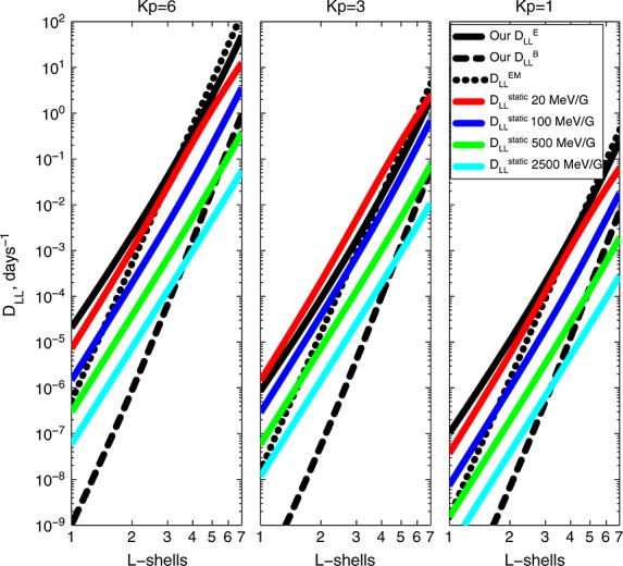
Comparison between our analytic electric and magnetic field diffusion coefficients,  and , with the electromagnetic
  and electrostatic
  diffusion coefficients presented in Brautigam and Albert [2000]. The black solid, dashed, and dotted lines represent
  ,
,  , and , respectively. The solid red, blue, green, and cyan lines represent the electrostatic diffusion coefficient,
  , for electrons with M values of 20 MeV/G, 100 MeV/G, 500 MeV/G, and 2500 MeV/G, respectively. These M values correspond to a 1 MeV electron in a dipole model of the Earth's magnetic field at L = 1.84, 3.15, 5.38, 6.78, and 9.21, respectively.
Interestingly, the electromagnetic diffusion coefficients  from Brautigam and Albert [2000] are only slightly higher than our
  values on L shells
  3. This agreement is surprising since ≳ is derived using the method from Fälthammar [1965] and only 1 month of ULF measurements, whereas
  is derived using the method from Brizard and Chan [2001] [see also Fei et al., 2006], and over 15 years of ULF wave measurements.
5. Statistical Variation of PSD Values
One assumption which has been made in the derivation of our electric and magnetic field diffusion coefficients is that the median PSDs provide a good representation of the expected PSD values. Of course, during individual time periods, the observed ULF wave spectra are likely to be more structured than the median spectral profiles, and likely over short time periods not represented by simple power law variations. In using the median spectra to specify the diffusion coefficients, one makes the assumption that the empirical ULF wave power spectra provide a good approximation to the longer time scale ensemble effect of multiple individual packets of ULF wave power when averaged within the quasi-linear (diffusive) radial transport approximation. However, to investigate the variability of the spectra within individual Kp bins one can also examine structure of the upper and lower quartiles of the distributions, rather than the median, representing the fact that there is variation in the distribution of the actual magnetic and electric field PSD values during time intervals with a specific value of Kp. Consequently, at a particular point in time the accuracy of our analytic expressions for  and
and  derived from these median PSD values will depend to some degree on the variability of the ULF wave power within a given Kp bin, and on how close the actual PSD values at that moment in time are to the median PSD values. In order to quantify the distribution of the PSD values in a given Kp bin, we calculated the upper and lower quartile PSD values in each Kp bin.
5.1. In Situ Compressional Magnetic PSD Statistics
Figure 6 illustrates the upper, lower, and median quartiles of compressional magnetic field PSD values binned with Kp, derived from our statistical database of 20 min data windows from GOES East and West data from 1996 to 2005. The solid blue, green, and black lines in Figure 6a represent the median compressional magnetic field PSD values from GOES East for Kp = 1, 3, and 6, respectively. The dashed lines above and below the solid lines represent the upper and lower quartile values, respectively. These results show that for Kp = 1, 3, and 6, the upper quartile and lower quartile PSD values are approximately a factor of 3 above and below the median PSD values. Significantly, they also show that the power spectral slope remains the same at the upper and lower quartiles as it is at the median and that Kp continues to nicely order the distributions. Figure 6b represents the ratio of the upper quartile PSD, median PSD, and lower quartile PSD values for Kp = 0, 1, 2, 3, 4, 5, and 6 for GOES East compressional wave power again showing clearly that the upper and lower quartile PSD values are approximately a factor of 3 above and below the median PSD values for all values of Kp. In the same format as Figures 6a and 6b, the magnetic field PSD results taken from GOES West are illustrated in Figures 6c and 6d, showing that the upper and lower quartile PSD values are again a factor of 3 above and below the median PSD values, respectively, independent of both Kp and frequency.
Figure 6.
(a) GOES East median (solid line) and upper and lower quartile (dashed lines) compressional magnetic field PSD for Kp = 1 (blue), Kp = 3 (green), and Kp = 6 (black); (b) GOES East PSD ratios of the upper quartile, median, and lower quartile showing a constant factor of 3 between quartiles independent of frequency and Kp; (c) Same format as Figure 6a for GOES West; (d) Same format as Figure 6b for GOES West.
The magnetic field diffusion coefficient is linearly dependent on the compressional magnetic field PSD as shown in equation (3). Consequently,  values corresponding to the upper and lower quartile PSD values can be approximated by increasing or decreasing our analytic expressional for
  given in equation (20) by a factor of 3, respectively. This gives an indication of the uncertainty within the empirically driven ULF wave diffusion model when it is driven by Kp, and which arises due to the range of ULF wave power which exists within a given Kp bin.
5.2. Ground Magnetometer PSD Statistics
The upper and lower quartile PSD values have also been determined from the database of hourly D-component magnetic field PSD binned with Kp, derived from ∼15 years of Canadian Array for Realtime Investigations of Magnetic Activity (CARISMA) and Sub-Auroral Magnetometer Network (SAMNET) ground magnetometer measurements. The solid blue, green, and black lines in Figure 7a illustrate median D-component PSD values for Kp = 1, 3, and 6, respectively, from the GILL station in the CARISMA array. The upper and lower quartile values are represented by the dashed lines above and below the solid lines. Figure 7b illustrates the ratio of the lower quartile, upper quartile, and median PSD values for Kp = 0, 1, 2, 3, 4, 5, and 6.The ratio of the lower quartile, upper quartile and median PSD values for Kp = 0, 1, 2, 3, 4, 5, and 6 at each of the other 7 CARISMA and SAMNET ground magnetometer stations from this study and from Ozeke et al. [2012a] (see that paper for more details) are also presented in Figure 8.
Figure 7.
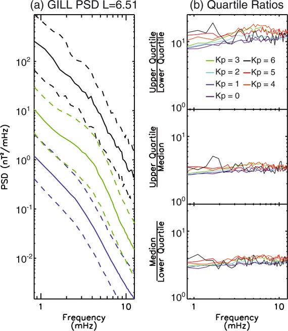
(a) The median, upper quartile, and lower quartile D-component magnetic field PSD measured at GILL derived from our database of PSD values binned with Kp. The purple, green, and black curves illustrate the median PSD values for Kp = 1, Kp = 3, and Kp = 6, respectively. The dashed curves above and below the solid curves represent the upper and lower quartile values of the PSD. (b) The ratio of the upper and lower quartile and median PSD values for Kp values from 0 to 6.
Figure 8.
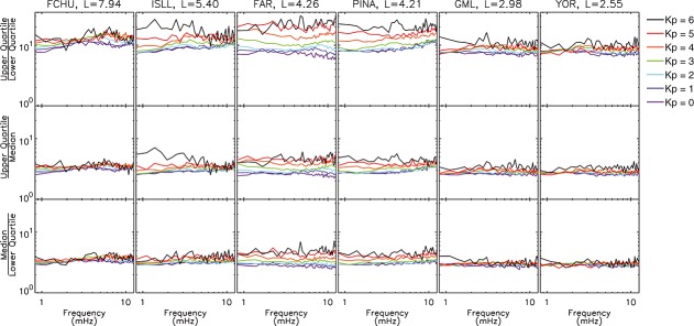
The ratio of the upper and lower quartile and median D-component magnetic field PSD values for Kp = 0, 1, 2, 3, 4, 5, and 6 at each of the remaining six selected ground magnetometer stations (data for GILL is shown in Figure 6).
Similar to the in situ GOES spacecraft measurements shown in Figure 6, the ground magnetometer D-component PSD statistics indicate that across all L shells and for all Kp values, the upper and lower quartile PSD values are approximately a factor of 3 above and below the median PSD values, as illustrated in Figures 7 and 8. Again, the data remain well-ordered by Kp. The equatorial electric field PSD values are proportional to the ground PSD values [see Ozeke et al., 2009, 2012a], and as shown in equation (2), the electric field diffusion coefficients are proportional to the equatorial electric field PSD values. Consequently, the  values are proportional to the ground PSD values, such that the upper and lower quartile PSD values can be approximated by increasing or decreasing our analytic expressions for
  given in equation (23) by a factor of 3, respectively.
6. Electron Flux Profiles From ULF Wave-Driven Radial Diffusion Model
The PSD statistics presented in Figures 6, 7, and 8 indicate that the lower and upper quartile PSD values are approximately a factor of 3 below and above the median PSD values, respectively. Since the diffusion coefficients are linearly proportional to the PSD values, multiplying the analytic expressions for the electric and magnetic field diffusion coefficient based on the median PSD values shown in equations (20) and (23) by a factor of 3 gives approximate expressions for the diffusion coefficients based on the upper quartile PSD values.
Similarly, dividing equations (20) and (23) by a factor of 3 gives approximate expressions for the diffusion coefficients based on the lower quartile PSD values. These expressions for the diffusion coefficients scaled up and down by a factor of 3 can be applied into data assimilation models of the radiation belts such as the DREAM model [Koller et al., 2007], where knowledge of the uncertainty in the physical parameters is included directly into the model using the Kalman filter algorithm.
Figures 9b and 10b show a comparison of the 90° 0.976 MeV differential electron flux measured by the CRRES MEA instrument over a period of ∼90 days with the equatorial differential electron flux produced by solving equation (1). Equation (1) is solved using our empirical expressions for the ULF wave-driven diffusion coefficients as a function of Kp based on the upper (Figures 9c and 10c), median (Figures 9d and 10d), and lower (Figures 9e and 10e) quartile PSD values. The values of the electron phase space density f at energies above and below 0.976 MeV at each point in the simulation from L = 7 to L = 1 were obtained by numerically solving equation (1) in a dipole magnetic field model. These electron phase space density values were converted into the 0.976 MeV equatorial differential electron flux J, using the relationship
| 25 |
Figure 9.
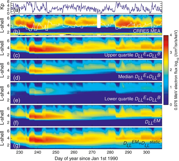
Comparison of the differential flux of 0.976 MeV electrons in 1990 measured by the CRRES Medium Electrons A (MEA) with those simulated using different diffusion coefficients and the electron lifetimes from Shprits et al. [2007] outside the plasmapause. Inside the plasmapause the electron lifetime is set to 10 days. (a) Time series of Kp; (b) CRRES MEA observed flux, with the plasmapause location represented by the white curve; (c) the diffusion model with 3 times higher DLL values than the analytic diffusion coefficients shown in equations (20) and (23), corresponding to the upper quartile PSD values; (d) the diffusion model with the analytic diffusion coefficient shown in equations (20) and (23) derived from the fits to the median PSD values; (e) the diffusion model with DLL values 3 times lower than the analytic diffusion coefficients shown in equations (20) and (23), corresponding to the lower quartile PSD values; (f) the diffusion model with the  values from Brautigam and Albert [2000]; and (g) the diffusion model with the and
  values from Brautigam and Albert [2000].
Figure 10.
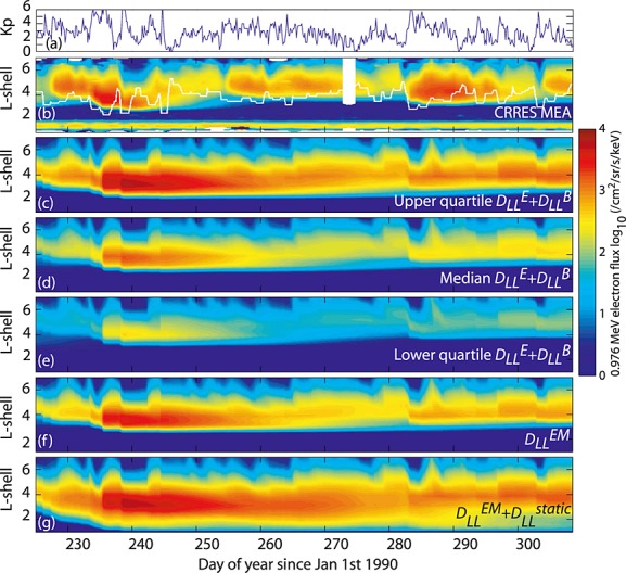
Comparison of the differential flux of 0.976 MeV electrons in 1990 measured by the CRRES MEA with those simulated using different diffusion coefficients. Outside the plasmapause the electron lifetimes are set to twice the values from Shprits et al. [2007], and inside the plasmapause the electron lifetime is set to 10 days. (a) Time series of Kp; (b) CRRES MEA observed flux, with the plasmapause location represented by the white curve; (c) the diffusion model with 3 times higher DLL values than the analytic diffusion coefficients shown in equations (20) and (23), corresponding to the upper quartile PSD values; (d) the diffusion model with the analytic diffusion coefficient shown in equations (20) and (23) derived from the fits to the median PSD values; (e) the diffusion model with DLL values 3 times lower than the analytic diffusion coefficients shown in equations (20) and (23), corresponding to the lower quartile PSD values; (f) the diffusion model with the  values from Brautigam and Albert [2000]; and (g) the diffusion model with the
  and
and  values from Brautigam and Albert [2000].
Here E and p are the kinetic energy and momentum of the electrons, respectively.
For comparison with the electron flux simulations derived using our  and
and  values we also calculate the electron flux using the electromagnetic diffusion coefficient
  (Figures 9f and 10f) and the sum of the electromagnetic plus the electrostatic diffusion coefficients
  (Figures 9g and 10g) taken from Brautigam and Albert [2000].
The outer boundary flux is specified at L = 7 from the CRRES MEA flux measurements at each of the MEA energy channels by taking the median electron flux value during each orbit over the time interval when the spacecraft is within 0.1 RE of L = 7. Examples of the electron flux used for the outer boundary condition over a 90 day period are illustrated in Figure 11. Note that for times between CRRES apogees, the data are interpolated in the model to provide outer boundary conditions with the hourly resolution of the radial diffusion model runs. At the inner boundary L = 1 we set the electron flux to be 0, representing loss to the ionosphere. Analytic expressions for the electron lifetime, τ outside the plasmasphere as a function of Kp, L shell and energy are given in Shprits et al. [2007], and these electron lifetimes are used to produce the results presented in Figure 9. However, Y. Y. Shprits (personal communication, 2013) state that these electron lifetimes need to be multiplied by a factor of 2, and we use these corrected electron lifetimes in the simulations illustrated in Figure 10. Inside the plasmasphere we set the electron lifetime, τ, to 10 days, which is the approach used in Shprits et al. [2005]. The plasmapause location is estimated using the approximation given in Carpenter and Anderson [1992]. The electron flux simulations are driven purely by the time series of Kp, which is shown in Figures 9a and 10a.
Figure 11.
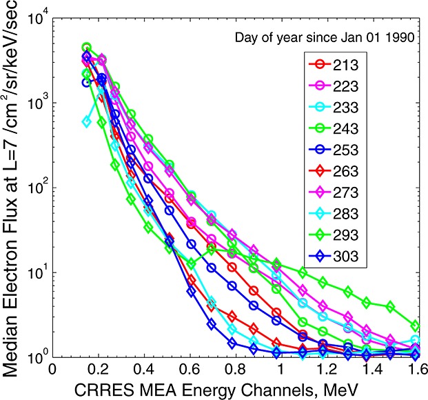
Median electron flux measured by the CRRES MEA instrument within 0.1 RE of L = 7 during each orbit. The symbols represent the electron flux measured at each energy channel at 10 day time intervals over a period of 90 days.
The results in both Figures 9 and 10 illustrate that the general features of the flux enhancements measured with the CRRES MEA are also very well reproduced in each of the diffusion simulations. Figures 9b and 10b show that the inner edge of the outer radiation belt approximately follows the location of the plasmapause, as was also noted in Li et al. [2001]. At ∼245 days the location of the plasmapause sharply jumps upward from L ∼ 2 to L ∼ 5, and the corresponding measured inner edge of the outer radiation belt also moves upward during the same interval; see Figures 9b and 10b. This rapid change in the flux as the plasmapause moves upward may indicate that the electron lifetime inside the plasmapause is short during this time interval causing the electron flux to rapidly decay in this region. However, the decrease in the electron flux inside the plasmapause at ∼245 days is not clearly shown in the simulations which may result from our assumed electron lifetime of 10 days inside the plasmapause being too long during this time interval. In future work, we will investigate what impact using different models for the electron lifetime has on the electron flux. However, this work is beyond the scope of this paper.
In general, the simulations in Figures 9c–9f and 10c–10f show a flux enhancement penetrating inward to L ∼ 3 during days 235–260 and moving back up to L = 4 during days 260–285 before finally moving slightly inward again—as also seen observationally in the CRRES MEA data. The intensity of the flux enhancements depends to some degree on the choice of diffusion coefficient used. However, all simulations in Figures 9c–9f and 10c–10f largely reproduce the qualitative structure seen by CRRES. Note also that there is also excellent quantitative agreement between the observed differential flux at 0.976 MeV and the results from the radial diffusion model—and no renormalization or other changes to the simulated flux have been applied. Given that the observed differential flux varies by more than 3 orders of magnitude, we consider this quantitative agreement to be rather impressive. In general, the measured electron flux values are between the electron flux values simulated using the upper and lower quartile PSDs. It is not unreasonable to hypothesize that there might be more ULF wave power at a given Kp during storm times than on average, which could explain the improved quantitative agreement using the PSD values greater than the median values. Figures 9f and 10f also illustrate that using only the  values from Brautigam and Albert [2000] and neglecting the
  term also produces an electron flux in good agreement with the measured flux. However, Figures 9g and 10g illustrate that inclusion of both the
  and the
  terms enhance the electron flux on L shells ≲ 4, producing a flux >100 times greater than that measured and shown in Figures 9b and 10b [see also Kim et al., 2011; Ozeke et al., 2012b].
7. Discussion and Conclusions
In this paper we have derived simple analytic expressions for both the electric (see equation (23)) and magnetic (see equation (20)) field radial diffusion coefficients based on observations of ULF wave power as a function of L and Kp. These can easily be incorporated in models of the Earth's radiation belts, and since we have shown that to a good approximation both the electric and magnetic diffusion coefficients are independent of first adiabatic invariant, they can also be very efficiently coded to produce models of differential flux as a function of L and time at fixed energy.
The empirical expressions presented here represent the median power spectral density (PSD) of the ULF waves and hence the median magnitude of the diffusion coefficients for a specific value of Kp. The actual value of the diffusion coefficients at a specific Kp value can of course vary from these median values. For example, in section 10 we showed that the diffusion coefficients derived from the upper and lower quartile PSD values are approximately a factor of 3 greater and lower than our analytic expressions for the diffusion coefficients based on the median, respectively. This simple scaling factor of 3 is remarkably constant across all L shells and Kp values, for both the electric and magnetic field diffusion coefficients, as illustrated in Figures 6, 7, and 8. Data from the quartiles can for example be used in data assimilation radiation belt models where knowing the uncertainties in the physics-based modules can be valuable for the filtering steps (e.g., within the SALAMMBO [Varotsou et al., 2008] model; S. Bourdaire (discussion at the AGU Chapman conference on Dynamics of the Earth's Radiation Belts and Inner Magnetosphere, personal communication, 2011). For 50% of the time the ULF electric and magnetic diffusion coefficients will lie between these upper and lower quartile values. However, for the other 50% of time the diffusion coefficients will be outside the range given by the upper and lower quartile values. For the comparison of model results with CRRES differential flux data at 1 MeV, the best agreement (qualitatively and quantitatively) was obtained using the upper quartile results—which might be explained physically if the larger wave power is generated at a specific Kp during storms which cause belt enhancements. Nonetheless, given that the differential electron flux in the outer belt varies by orders of magnitude, and there is only a factor of 3 difference in diffusion coefficient magnitude between either upper or lower quartile and the median, the agreement in model belt morphology (cf. Figures 9 and 10) remains quite good for all three (upper, lower quartile, and median) representations of Kp-driven ULF wave radial diffusion coefficient.
Interestingly, there are significant physical implications for the structure of the outer radiation belt due to the first invariant independence of the radial diffusion coefficients we have shown here. Indeed, given this M independence of the diffusion coefficients, it is obvious in the context of radial transport that the time dependence of the energy spectra and differential flux of the source population at the outer boundary play a critical role in determining the structure of the belts. This is especially true if the belts are observed to have (L time) structure which varies with energy. Figure 11 shows the differential energy spectra at L = 7 used to drive the radial diffusion results shown in Figures 9 and 10. In Figure 11 the CRRES energy spectra are shown every 10 days to illustrate the variability in the outer boundary condition which results in the model 0.976 MeV electron differential flux profiles in Figures 9 and 10. Of course, any transport and acceleration will also be competing with loss processes which themselves can also have strong energy, L shell, and activity (e.g., Kp) dependence.
In Figures 9 and 10, which includes the empirical L, energy and Kp-dependent loss outside the plasmapause arising from chorus waves based on Shprits et al. [2007], there is excellent agreement between the belt structure produced by radial transport using the Kp-driven radial diffusion coefficients presented here and the CRRES observations at around 1 MeV. This points to the potential importance of the diffusion coefficient model and suggests it might provide excellent utility when incorporated into the radial diffusion modules of radiation belt models. It is also interesting to note that at 1 MeV, and on this 90 day time scale, there is good agreement between the model and the data especially in relation to belt activations and the location of the inner boundary of the belt. This is despite the fact that the radial diffusion model does not explicitly include any local acceleration source such as might arise from resonance with lower band VLF chorus [e.g., Meredith et al., 2003; Chen et al., 2007]. The model results also do not include any effects from magnetopause shadowing and resulting outward radial diffusion [e.g., Loto'aniu et al., 2010; Turner et al., 2012]. In future developments of the model, such shadowing losses, based, for example, on a solar wind parameter-driven location of the magnetopause, could also be incorporated. This might further improve the agreement between the model and the CRRES observations at the outer edge of the belt especially during time periods which rely on interpolation between the observed spectra at the outer boundary condition, for example, in between CRRES apogees in the time period shown in Figures 9 and 10.
An alternative approach to using empirical Kp dependence of the ULF wave-driven radial diffusion coefficients is to use the observed ULF wave power seen during specific storm intervals as a function of L to determine the coefficients again using equations (2) and (3). This might represent an alternative, potentially more accurate, approach for modeling diffusion coefficient values over a specific interval of time. In situ measurements of the ULF wave PSD measured by a single satellite only provide the PSD at a single L shell at each point in time. To determine the required PSD as a function of L shell at each point in time would require the deployment of multisatellite constellations in the magnetic equatorial plane measuring the spatial and temporal variations of the ULF wave PSD, as discussed in Brautigam et al. [2005]. Alternatively, ground magnetometer networks can be used to measure the spatial and temporal variations in the PSD on the ground and these values can then be mapped into space to give the required electric field PSD values in the magnetic equatorial plane as a function of L shell at each point in time. This approach might provide more accurate values for the electric field diffusion coefficients than those based on the median or the upper and lower quartile PSD values from our statistical database of PSD values binned with Kp. However, this approach cannot be used to determine the compressional magnetic field diffusion coefficients since there is no established method for determining the compressional magnetic field PSD in the equatorial plane from ground magnetometer measurements.
In Ozeke et al. [2012b] the electron flux was determined by solving the diffusion equation with  and with
  . However, as described by these authors,
  is much smaller than
  , such that
  can generally be neglected in comparison to
  to very good accuracy. These results presented by Ozeke et al. [2012b] indicated that the electron flux can be accurately simulated using only the electric field radial diffusion coefficient and that inclusion of
  had negligible effect on the electron flux [see Ozeke et al., 2012b, Figure 6]. The neglect of the magnetic diffusion term in comparison to the electric field term determined from data by Ozeke et al. [2012a, 2012b] is also in agreement with the same conclusion drawn by Tu et al. [2012] using model results from the Lyon-Fedder-Mobarry magnetohydrodynamic code [Lyon et al., 2004]. Interestingly, from a practical perspective, this also provides a pragmatic solution to the problem also discussed by Ozeke et al. [2012b] that if the electric and magnetic fields in the ULF wave modes which are driving diffusion are correlated, for example, through Faraday's Law, then there could potentially be a violation of the Brizard and Chan [2001] assumption that the fields are uncorrelated and hence that the diffusion terms can be combined additively [see also Perry et al., 2005, 2006]. However, since we have shown here that the magnetic term can be neglected, accurate diffusion runs can be completed using only the electric field diffusion term presented here in equation (23).
In future work, we intend to compare the electron differential flux observed during storm events with that derived using a radial diffusion model driven using the empirical ULF wave-derived diffusion coefficients presented here. This can also be compared to the diffusion derived using observed electric field PSD values derived from actual ground magnetometer magnetic field PSD measurements, and where available also derived from satellite electric field observations. We believe that the analytic empirical diffusion coefficient expressions presented here allow for differences between the upper and lower quartile PSD values and the median to be included in data assimilation models and represent a significant improvement over using the diffusion coefficients presented in Brautigam and Albert [2000] which are currently used in almost all radiation belt models. Moreover, using the improved ULF wave radial diffusion coefficients we have presented here in radiation belt models is now particularly important as we strive to understand the dominant physical mechanisms which are responsible for relativistic electron flux variability through model comparisons with the in situ measurements from the recently launched NASA Van Allen Probes mission [e.g., Reeves, 2007].
Acknowledgments
I.R. Mann is supported by a Discovery Grant from Canadian NSERC. This work is supported by the Canadian Space Agency. We acknowledge the WDC for Geomagnetism, Kyoto University, Japan, for the geomagnetic indices, and CDAWeb for GOES, CRRES MEA, and solar wind speed data. The CANOPUS magnetometer array (now CARISMA http://www.carisma.ca) is operated by the University of Alberta and funded by the Canadian Space Agency. The U.K. Sub-Auroral Magnetometer Network (SAMNET) is operated by the Space Plasma Environment and Radio Science (SPEARS) group, Department of Physics, Lancaster University. We acknowledge NASA contract NAS5-02099 and V. Angelopoulos for use of data from the THEMIS Mission. Specifically K. H. Glassmeier, U. Auster, and W. Baumjohann for the use of FGM data provided under the lead of the Technical University of Braunschweig and with financial support through the German Ministry for Economy and Technology and the German Center for Aviation and Space (DLR) under contract 50 OC 0302. This work was supported in part by participation in the MAARBLE (Monitoring, Analyzing and Assessing Radiation Belt Loss and Energization) consortium. MAARBLE has received funding from the European Community's Seventh Framework Programme (FP7-SPACE-2010-1, SP1 Cooperation, Collaborative project) under grant agreement 284520. This paper reflects only the authors' views, and the European Union is not liable for any use that may be made of the information contained herein.
Robert Lysak thanks Jay Albert and an anonymous reviewer for their assistance in evaluating this paper.
References
- Baker DN, Blake JB, Callis LB, Cummings JR, Hovestadt D, Kanekal S, Klecker B, Mewaldt RA. Zwickl RD. Relativistic electron acceleration and decay time scales in the inner and outer radiation belts: Sampex. Geophys. Res. Lett. 1994;21(6):409–412. doi: 10.1029/93GL03532. [Google Scholar]
- Beutier T. Boscher D. A three-dimensional analysis of the electron-radiation belt by the Salammbo Code. J. Geophys. Res. 1995;100(A8):14,853–14,861. doi: 10.1029/94JA03066. [Google Scholar]
- Blake JB, Kolasinski WA, Fillius RW. Mullen EG. Injection of electrons and protons with energies of tens of MeV into L < 3 on 24 March 1991. Geophys. Res. Lett. 1992;19(8):821–824. doi: 10.1029/92GL00624. [Google Scholar]
- Brautigam DH. Albert JM. Radial diffusion analysis of outer radiation belt electrons during the October 9, 1990, magnetic storm. J. Geophys. Res. 2000;105(A1):291–309. [Google Scholar]
- Brautigam DH, Ginet GP, Albert JM, Wygant JR, Rowland DE, Ling A. Bass J. CRRES electric field power spectra and radial diffusion coefficients. J. Geophys. Res. 2005;110:A02214. doi: 10.1029/2004JA010612. [Google Scholar]
- Brizard AJ. Chan AA. Relativistic bounce-averaged quasilinear diffusion equation for low-frequency electromagnetic fluctuations. Phys. Plasmas. 2001;8(11):4762–4771. [Google Scholar]
- Carpenter DL. Anderson RR. An ISEE/whistler model of equatorial electron density in the magnetosphere. J. Geophys. Res. 1992;97(A2):1097–1108. doi: 10.1029/91JA01548. [Google Scholar]
- Chen Y, Reeves GD. Friedel RHW. The energization of relativistic electrons in the outer Van Allen radiation belt. Nat. Phys. 2007;3:614–617. doi: 10.1038/nphys655. [Google Scholar]
- Cornwall JM. Diffusion processes influenced by conjugate-point wave phenomena. Radio Sci. 1968;3(7):740–744. [Google Scholar]
- Elkington SR, Chan AA, et al. Wiltberger M. Global structure of ULF waves during the 24–26 September 1998 geomagnetic storm. In: Summers D, editor; Dynamics of the Earth's Radiation Belts and Inner Magnetosphere Geophys. Monogr. Ser. Vol. 199. Washington, D. C: AGU; 2012. pp. 127–138. doi: 10.1029/2012GM001348. [Google Scholar]
- Fälthammar CG. Effects of time-dependent electric fields on geomagnetically trapped radiation. J. Geophys. Res. 1965;70(11):2503–2516. doi: 10.1029/JZ070i011p02503. [Google Scholar]
- Fei Y, Chan AA, Elkington SR. Wiltberger MJ. Radial diffusion and MHD particle simulations of relativistic electron transport by ULF waves in the September 1998 storm. J. Geophys. Res. 2006;111:A12209. doi: 10.1029/2005JA011211. [Google Scholar]
- Glassmeier K-H. On the influence of ionospheres with non-uniform conductivity distribution on hydromagnetic waves. J. Geophys. 1984;54:125–137. [Google Scholar]
- Horne RB, Thorne RM, Glauert SA, Albert JM, Meredith NP. Anderson RR. Timescale for radiation belt electron acceleration by whistler mode chorus waves. J. Geophys. Res. 2005;110:A03225. doi: 10.1029/2004JA010811. [Google Scholar]
- Huang C, Spence HE, Hudson MK. Elkington SR. Modeling radiation belt radial diffusion in ULF wave fields: 2. Estimating rates of radial diffusion using combined MHD and particle codes. J. Geophys. Res. 2010;115:A06216. doi: 10.1029/2009JA014918. [Google Scholar]
- Hughes WJ. Southwood DJ. Screening of micropulsation signals by atmosphere and ionosphere. J. Geophys. Res. 1976;81(19):3234–3240. doi: 10.1029/JA081i019p03234. [Google Scholar]
- Kim K-C, Shprits Y, Subbotin D. Ni B. Understanding the dynamic evolution of the relativistic electron slot region including radial and pitch angle diffusion. J. Geophys. Res. 2011;116:A10214. doi: 10.1029/2011JA016684. [Google Scholar]
- Koller J, Chen Y, Reeves GD, Friedel RHW, Cayton TE. Vrugt JA. Identifying the radiation belt source region by data assimilation. J. Geophys. Res. 2007;112:A06244. doi: 10.1029/2006JA012196. [Google Scholar]
- Lanzerotti LJ. Morgan CG. ULF geomagnetic power near L=4.2. Temporal variation of radial diffusion-coefficient for relativistic electrons. J. Geophys. Res. 1973;78(22):4600–4610. doi: 10.1029/JA078i022p04600. [Google Scholar]
- Li XL, Roth I, Temerin M, Wygant JR, Hudson MK. Blake JB. Simulation of the prompt energization and transport of radiation belt particles during the March 24, 1991 SSC. Geophys. Res. Lett. 1993;20(22):2423–2426. doi: 10.1029/93GL02701. [Google Scholar]
- Li X, Baker DN, Kanekal SG, Looper M. Temerin M. Long term measurements of radiation belts by SAMPEX and their variations. Geophys. Res. Lett. 2001;28:3827–3830. doi: 10.1029/2001GL013586. [Google Scholar]
- Loto'aniu TM, Singer HJ, Waters CL, Angelopoulos V, Mann IR, Elkington SR. Bonnell JW. Relativistic electron loss due to ultralow frequency waves and enhanced outward radial diffusion. J. Geophys. Res. 2010;115:A12245. doi: 10.1029/2010JA015755. [Google Scholar]
- Lyon JG, Fedder JA. Mobarry CM. The Lyon-Fedder-Mobarry (LFM) global MHD magnetospheric simulation code. J. Atmos. Sol. Terr. Phys. 2004;66(15–16):1333–1350. doi: 10.1016/j.jastp.2004.03.020. [Google Scholar]
- Meredith NP, Cain M, Horne RB, Thorne RM, Summers D. Anderson RR. Evidence for chorus-driven electron acceleration to relativistic energies from a survey of geomagnetically-disturbed periods. J. Geophys. Res. 2003;108(A6):1248. doi: 10.1029/2002JA009764. [Google Scholar]
- Ozeke LG, Mann IR. Rae IJ. Mapping guided Alfven wave magnetic field amplitudes observed on the ground to equatorial electric field amplitudes in space. J. Geophys. Res. 2009;114:A01214. doi: 10.1029/2008JA013041. [Google Scholar]
- Ozeke LG, Mann IR, Murphy KR, Rae IJ, Milling DK, Elkington SR, Chan AA. Singer HJ. ULF wave derived radiation belt radial diffusion coefficients. J. Geophys. Res. 2012a;117:A04222. doi: 10.1002/2013JA019204. doi: 10.1029/2011JA017463. [DOI] [PMC free article] [PubMed] [Google Scholar]
- Ozeke LG, Mann IR, Murphy KR, Rae IJ, et al. Chan AA. ULF wave-driven radial diffusion simulation of the outer radiation belt. In: Summers D, editor; Dynamics of the Earth's Radiation Belts and Inner Magnetosphere Geophys. Monogr. Ser. Vol. 199. Washington, D. C: AGU; 2012b. pp. 139–149. doi: 10.1029/2012GM001332. [Google Scholar]
- Perry KL, Hudson MK. Elkington SR. Incorporating spectral characteristics of Pc5 waves into three-dimensional radiation belt modeling and the diffusion of relativistic electrons. J. Geophys. Res. 2005;110:A03215. doi: 10.1029/2004JA010760. [Google Scholar]
- Perry KL, Hudson MK. Elkington SR. Correction to “Incorporating spectral characteristics of Pc5 waves into three-dimensional radiation belt modeling and the diffusion of relativistic electrons”. J. Geophys. Res. 2006;111:A11228. doi: 10.1029/2006JA012040. [Google Scholar]
- Rae IJ, Mann IR, Murphy KR, Ozeke LG, Milling DK, Chan AA, Elkington SR. Honary F. Ground-based magnetometer determination of in situ Pc4–5 ULF electric field wave spectra as a function of solar wind speed. J. Geophys. Res. 2012;117:A04221. doi: 10.1029/2011JA017335. [Google Scholar]
- Reeves G. Radiation belt storm probes: A new mission for space weather. Space Weather. 2007;5:S11002. doi: 10.1029/2007SW000341. [Google Scholar]
- Sarris T, Li X. Temerin M. Simulating radial diffusion of energetic (MeV) electrons through a model of fluctuating electric and magnetic fields. Ann. Geophys. 2006;24:2583–2598. doi: 10.5194/angeo-24-2583-2006. [Google Scholar]
- Schulz M. Lanzerotti LJ. Particle Diffusion in the Radiation Belts Physics and Chemistry in Space. Vol. 7. New York Heidelberg Berlin: Springer-Verlag; 1974. p. 215. [Google Scholar]
- Shprits YY, Thorne RM, Reeves GD. Friedel R. Radial diffusion modeling with empirical lifetimes: Comparison with CRRES observations. Ann. Geophys. 2005;23:1467–1471. doi: 10.5194/angeo-23-1467-2005. [Google Scholar]
- Shprits YY, Thorne RM, Reeves GD. Friedel R. Radial diffusion modeling with empirical lifetimes: Comparison with CRRES observations. Ann. Geophys. 2007;23(4):1467–1471. [Google Scholar]
- Southwood DJ. Kivelson MG. Charged-particle behavior in low-frequency geomagnetic-pulsations.2. graphical approach. J. Geophys. Res. 1982;87(NA3):1707–1710. [Google Scholar]
- Subbotin DA. Shprits YY. Three-dimensional modeling of the radiation belts using the Versatile Electron Radiation Belt (VERB) code. Space Weather. 2009;7:S10001. doi: 10.1029/2008SW000452. [Google Scholar]
- Takahashi K. Anderson BJ. Distribution of ULF Energy (f < 80 Mhz) in the Inner Magnetosphere: A statistical analysis of AMPTE CCE magnetic field data. J. Geophys. Res. 1992;97(A7):10,751–10,773. doi: 10.1029/92JA00328. [Google Scholar]
- Tu W, Elkington SR, Li X, Liu W. Bonnell J. Quantifying radial diffusion coefficients of radiation belt electrons based on global MHD simulation and spacecraft measurements. J. Geophys. Res. 2012;117:A10210. doi: 10.1029/2012JA017901. [Google Scholar]
- Turner DL, Shprits Y, Hartinger M. Angelopoulos V. Explaining sudden losses of outer radiation belt electrons during geomagnetic storms. Nat. Phys. 2012;8:208–212. doi: 10.1038/nphys2185. [Google Scholar]
- Varotsou A, Boscher D, Bourdarie S, Horne RB, Meredith NP, Glauert SA. Friedel RH. The Salammbo 3D electron radiation belt physical model: Test simulations including electron-chorus resonant interactions. J. Geophys. Res. 2008;113:A12202. doi: 10.1029/2007JA0128262. [Google Scholar]
- Yoshikawa A. Itonaga M. The nature of reflection and mode conversion of MHD waves in the inductive ionosphere: Multistep mode conversion between divergent and rotational electric fields. J. Geophys. Res. 2000;105(A5):10,565–10,584. doi: 10.1029/1999JA000159. [Google Scholar]