Pathway Graphical Lasso

Abstract

Graphical models provide a rich framework for summarizing the dependencies among variables. The graphical lasso approach attempts to learn the structure of a Gaussian graphical model (GGM) by maximizing the log likelihood of the data, subject to an l₁ penalty on the elements of the inverse co-variance matrix. Most algorithms for solving the graphical lasso problem do not scale to a very large number of variables. Furthermore, the learned network structure is hard to interpret. To overcome these challenges, we propose a novel GGM structure learning method that exploits the fact that for many real-world problems we have prior knowledge that certain edges are unlikely to be present. For example, in gene regulatory networks, a pair of genes that does not participate together in any of the cellular processes, typically referred to as pathways, is less likely to be connected. In computer vision applications in which each variable corresponds to a pixel, each variable is likely to be connected to the nearby variables. In this paper, we propose the pathway graphical lasso, which learns the structure of a GGM subject to pathway-based constraints. In order to solve this problem, we decompose the network into smaller parts, and use a message-passing algorithm in order to communicate among the subnetworks. Our algorithm has orders of magnitude improvement in run time compared to the state-of-the-art optimization methods for the graphical lasso problem that were modified to handle pathway-based constraints.

1 Introduction

Gaussian graphical models (GGMs) provide a compact representation of the statistical dependencies among variables. Learning the structure of GGMs from data that contain the measurements on a set of variables across samples has significantly facilitated data-driven discovery in a diverse set of scientific fields. For example, biologists can gain insights into how thousands of genes interact with each other in various disease processes by learning the GGM structure from gene expression data that measure the mRNA expression levels of genes across hundreds of patients. Existing algorithms for learning the structure of GGMs lack scalability and interpretability, which limits their utility when there is a large number of variables. Most learning algorithms perform O(p³) computations per iteration, where p denotes the number of variables; consequently they are impractical when p exceeds tens of thousands. Furthermore, a network based on a large number of variables can be difficult to interpret due to the presence of a large number of connections between the variables.

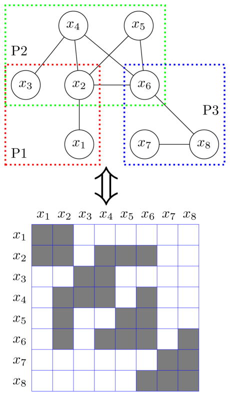
To resolve these challenges, we propose the pathway graphical lasso (PathGLasso) framework, which consists of the incorporation of pathway-based constraints and an efficient learning algorithm. We assume that we are given a set of pathways a priori, and that each pathway contains a (possibly overlapping) subset of the variables. We assume that a pair of variables can be connected to each other only if they co-occur in at least one pathway. Figure 1 illustrates a simple example network of 8 variables: {x₁, x₂, x₃} in Pathway 1, {x₂, x₃, x₄, x₅, x₆} in Pathway 2 and {x₆, x₇, x₈} in Pathway 3. By incorporating the pathway constraints, we can effectively reduce the search space of network structures by excluding nonsensical edges.

Figure 1.

Graphical representation of pathways (top) and the corresponding precision matrix (bottom).

Pathway constraints have the potential to improve structure learning of GGMs in several applications. In the context of gene regulatory networks, one can make use of pathway databases such as Reactome (Croft et al. 2011) that specify sets of genes that are likely work together. Making use of such pathways in learning the network can yield results that are more meaningful and interpretable. In computational neuroscience, when learning an interaction network of brain activation from fMRI data, we can use our prior knowledge that nearby brain regions are likely to interact with each other (Felleman and Van Essen 1991). In computer vision, in which each pixel in an image corresponds to a variable in a network, one can generate overlapping pathways by grouping nearby pixels; this has been shown to be an effective prior in several applications (Honorio et al. 2009). For example, Figure 2 compares network estimates of the true 2D lattice network for the unconstrained graphical lasso model and the pathway constrained graphical lasso model (2) when each pathway contains nearby variables.

Figure 2.

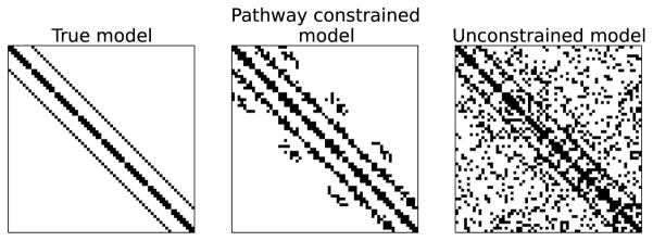
Comparison of learned networks between the pathway graphical lasso (middle) and the standard graphical lasso (right). The true network has the lattice structure (left).

The key idea in this paper is that we define certain edges to be non-existent only when the corresponding variables are not together in any of the pathways. Many of the potential edges within a pathway can also end up becoming zero. The pathway constraints provide a way of reducing the search space of structure learning. They do not determine the structure to a large extent.

In this paper, we present a learning algorithm that takes advantage of the pathway assumption in order to deliver a dramatic improvement in performance relative to existing approaches. We make use of a block-coordinate descent approach, in which we update each pathway individually. We apply a message-passing algorithm in order to enforce the correct solution jointly across all pathways.

The implementation of PathGLasso and example data are available at: http://pathglasso-leelab.cs.washington.edu/.

2 Pathway Constrained Sparse Inverse Covariance Estimation

2.1 Preliminaries

Suppose that we wish to learn a GGM with p variables based on n observations ${\mathbf{x}}^1,\dots ,{\mathbf{x}}^n\stackrel{\mathrm{i}.\mathrm{i}.\mathrm{d}.}{\sim }N(\mathbf{0},\mathbf{\sum })$, where Σ is a p × p covariance matrix. It is well known that (Σ⁻¹)_jj′ = 0 for some j ≠ j′ if and only if X_j and X_j′ are conditionally independent given X_k with k = {1, …, p}\{j, j′} (Mardia, Kent, and Bibby 1979; Lauritzen 1996). Hence, the non-zero pattern of Σ⁻¹ corresponds to the graph structure of a GGM. In order to obtain a sparse estimate for Σ⁻¹, a number of authors have considered the graphical lasso optimization problem (Yuan and Lin 2007; Banerjee, El Ghaoui, and d’Aspremont 2008; Friedman, Hastie, and Tibshirani 2007):

$$\begin{array}{l}\underset{\mathrm{\Theta }}{\text{minimize}}-logdet(\mathrm{\Theta })+\text{trace}(S\mathrm{\Theta })+\lambda {\Vert \mathrm{\Theta }\Vert }_1\\ \text{subject}\text{to}\mathrm{\Theta }\succcurlyeq 0,\end{array}$$ (1)

where S is the empirical covariance matrix and λ > 0 is an l₁ regularization parameter. We denote the estimate of the inverse covariance matrix by Θ throughout the paper.

2.2 Pathway Graphical Lasso Problem

Consider a set of edges within k pathways $P_1,\dots ,P_k:\mathcal{F}={\cup }_{t=1}^k\{(i,j)\mid i,j\in P_t\}$. We assume that edges that are outside of are set to zero. This modifies the graphical lasso problem (1) as:

$$\begin{array}{ll}\underset{\mathrm{\Theta }}{\text{minimize}}& -logdet(\mathrm{\Theta })+\text{trace}(S\mathrm{\Theta })+\lambda {\Vert \mathrm{\Theta }\Vert }_1\\ \text{subject}\text{to}& {\mathrm{\Theta }}_{ij}=0,(i,j)\notin \mathcal{F};\mathrm{\Theta }\succcurlyeq 0.\end{array}$$ (2)

To the best of our knowledge, this is a novel problem, and none of the existing algorithms for learning GGMs can solve (2) directly. However, many existing approaches for solving (1) either support (e.g., QUIC) or can easily be adapted to support (e.g., HUGE) a per-variable regularization scheme. Setting specific regularization parameter values in (1) to some very large number (say 10¹⁰) effectively forces the corresponding values in Θ to be zero. We observed in our experiments that methods that employ active set heuristics can get a significant performance boost from such a setting.

2.3 Related Work

Our proposal, PathGLasso, decomposes the original problem (2) into a set of smaller overlapping problems, and uses a divide-and-conquer approach to optimize the local marginal likelihood with a modified sparsity-inducing penalty. This novel combination of ideas differentiates PathGLasso from previous approaches to learn GGMs.

Several authors attempted to optimize the local marginal likelihood of a handful of nearby variables for parameter estimation in GGMs with fixed structures (Wiesel and Hero 2012; Meng et al. 2013). It was proven that this type of local parameter estimation produces a globally optimal solution under certain conditions (Mizrahi, Denil, and de Freitas 2014). Though these papers adopted a similar idea of exploiting the conditional independence of a set of variables from the rest of the network given their Markov blanket, they solve a fundamentally different problem. PathGLasso learns a pathway-constrained structure of the network in addition to estimating individual parameters. Moreover, the l₁ regularization that we employ for structure learning makes these previous approaches inapplicable to our setting.

Another approach (Hsieh et al. 2012) first partitions variables into non-overlapping pathways by using a clustering algorithm, and then estimates a network for each pathway. In contrast, in this paper we assume that overlapping pathway information is provided to us, although it could alternatively be estimated from the data, for example by running a clustering algorithm with soft assignment. The approach of (Hsieh et al. 2012) is not applicable to our problem, because combining independently estimated networks from overlapping pathways into a global network can lead to a non-positive definite solution. Like (Hsieh et al. 2012), PathGLasso is agnostic of the specific optimization algorithm for learning the network within each pathway.

There are methods that aim to infer modules, sets of densely connected variables. Many approaches attempt to learn a network with a prior that induces modules (Ambroise, Chiquet, and Matias 2009), which makes it significantly less efficient than without the prior. To address this, (Celik, Logsdon, and Lee 2014) proposed a method that can jointly learn modules and a network among modules. Although this method achieves scalability and interpretability, it does not learn a network of individual variables. PathGLasso addresses both of these shortcomings.

Finally, a number of methods have been proposed to solve the l₁ penalized sparse inverse covariance estimation problem (1). One such algorithm (Friedman, Hastie, and Tibshirani 2007) uses row-wise updates on the dual problem by solving a lasso problem at every step. The lasso problem is solved using a coordinate-descent algorithm that takes advantage of an active set heuristic, reducing computational load for sparse matrices. In Section 4, we provide a comparison to an efficient implementation of this method, provided by the R package HUGE (Zhao et al. 2012). Another paper (Hsieh et al. 2011) proposes a quadratic approximation based algorithm (QUIC) that achieves super-linear convergence rates as well as significant performance improvements due to clever partitioning of variables into free and fixed sets.

In the following section, we propose a novel learning algorithm for pathway constrained sparse inverse covariance estimation, and demonstrate that it shows significant improvement in run time compared to general off-the-shelf methods for (1) that we modified to solve (2).

3 PathGLasso Learning Algorithm

3.1 Overview

We employ a version of the block-coordinate descent approach to solve the optimization problem (2); a discussion of the convergence properties of the standard block-coordinate descent is provided in (Tseng 2001). In each iteration, we update the parameters that correspond to one pathway, with all of the other parameters held fixed. Consider updating the parameters in the pathway P₁. After re-arranging the variables, the p × p inverse covariance matrix Θ takes the form:

$$\mathrm{\Theta }=\left(\begin{array}{ccc}A& B& 0\\ B^T& C& D\\ 0& D^T& E\end{array}\right)$$ (3)

where ${\mathrm{\Theta }}_1=\left(\begin{array}{cc}A& B\\ B^T& C\end{array}\right)$ contains the parameters in P₁, ${\mathrm{\Theta }}_2=\left(\begin{array}{cc}C& D\\ D^T& E\end{array}\right)$ contains the parameters in the rest of the pathways, and C corresponds to the subset of variables that are in the intersection of P₁ and all other pathways.

3.2 Updating Each Pathway

We show that updating the parameters in P₁ with all of the other parameters held fixed boils down to estimating a p₁ × p₁ inverse covariance matrix, where p₁ is the number of variables in P₁. This is not obvious, because P₁ overlaps with other pathways (C in (3)). To update the parameters in P₁, we need to solve the following optimization problem:

$$\begin{array}{l}\underset{A,B,C}{\text{minimize}}-logdet(\mathrm{\Theta })+\text{trace}(S\mathrm{\Theta })+\lambda {\Vert \mathrm{\Theta }\Vert }_1\\ \text{subject}\text{to}\mathrm{\Theta }\succcurlyeq 0.\end{array}$$ (4)

Applying the Schur complement decomposition, we obtain

$$det\mathrm{\Theta }=detE·det({\mathrm{\Theta }}_1-\mathrm{\Delta }),$$ (5)

where

$$\mathrm{\Delta }=[\begin{array}{cc}0;& D\end{array}]·E^{-1}·[\begin{array}{cc}0& D^T\end{array}].$$ (6)

Given that D and E are fixed, the optimization problem (4) is equivalent to the following problem:

$$\begin{array}{l}\underset{{\mathrm{\Theta }}_1}{\text{minimize}}-logdet({\mathrm{\Theta }}_1-\mathrm{\Delta })+\text{trace}(S_1({\mathrm{\Theta }}_1-\mathrm{\Delta }))+\lambda {\Vert {\mathrm{\Theta }}_1\Vert }_1\\ \text{subject}\text{to}{\mathrm{\Theta }}_1-\mathrm{\Delta }\succcurlyeq 0,\end{array}$$ (7)

where S₁ is the portion of the empirical covariance matrix corresponding to P₁.

Let Ω = Θ₁ − Δ. Since our estimate of Θ is always positive definite, E is also positive definite as it is the principal submatrix of Θ. Thus, constraining Ω to be positive definite will guarantee the positive definiteness of Θ. Then, (7) is equivalent to the following optimization problem:

$$\begin{array}{l}\underset{\mathrm{\Omega }}{\text{minimize}}-logdet(\mathrm{\Omega })+\text{trace}(S_1\mathrm{\Omega })+\lambda {\Vert \mathrm{\Omega }+\mathrm{\Delta }\Vert }_1\\ \text{subject}\text{to}\mathrm{\Omega }\succcurlyeq 0.\end{array}$$ (8)

Note that (8) is the graphical lasso problem with a “shifted” l₁ penalty. This means that our block-coordinate update can make use of any algorithm for solving the graphical lasso problem, as long as it can be adapted to work with the shifted penalty. In this paper, we used the DP-GLASSO (dual-primal graphical lasso) algorithm (Mazumder, Hastie, and others 2012), which works well with restarts and guarantees a positive definite solution at each iteration.

3.3 Probabilistic Interpretation

The marginal distribution of the variables that are in P₁ is Gaussian with mean zero and precision matrix $\mathrm{\Omega }=\left(\begin{array}{cc}A& B\\ B^T& C-D·E^{-1}·D^T\end{array}\right)$, where Θ denotes the true precision matrix of the entire distribution partitioned as in (3). Then, the optimization problem (8) can be viewed as maximizing the marginal likelihood of the variables in P₁ with adjustments in the regularization term. That term makes it possible to take into account the variables that are outside of P₁. For example, in Figure 1, even if x₂ and x₃ are separately connected with x₄, maximizing the marginal likelihood of P₁ would induce an edge between x₂ and x₃ because x₄ is outside of P₁. Δ in (8) informs the algorithm that the connection between x₂ and x₃ can be explained away by x₄ when optimizing the marginal likelihood of P₁.

3.4 Marginalization of More Than One Pathway

In Section 3.2, we showed that updating the parameters for a given pathway requires the computation of Δ (6), a function of all of the other pathways. We could compute Δ directly by inverting a potentially very large matrix E (3), and performing two matrix multiplications. This corresponds to marginalizing all other pathways at once. In this section, we show that when more than two pathways are present, it is possible to avoid computing the matrix inverse of E explicitly, by instead marginalizing the pathways one-at-a-time.

As an example, we consider a very simple case of three pathways that form a linear chain,

$$\mathrm{\Theta }=\left(\begin{array}{cccc}A& B& 0& 0\\ B^T& C& D& 0\\ 0& D^T& E& F\\ 0& 0& F^T& G\end{array}\right).$$ (9)

Suppose that we want to update the top left pathway, corresponding to the matrix ${\mathrm{\Theta }}_1=\left(\begin{array}{cc}A& B\\ B^T& C\end{array}\right)$. Following the arguments in Section 3.2, computing (6) involves inverting the matrix $\left(\begin{array}{cc}E& F\\ F^T& G\end{array}\right)$. Instead, we note that

$$\begin{array}{l}det\mathrm{\Theta }=det(G)·det\left(\begin{array}{ccc}A& B& 0\\ B^T& C& D\\ 0& D^T& E-F{G}^{-1}{F}^T\end{array}\right)\\ =det(G)·det(E-F{G}^{-1}{F}^T)·det\left(\begin{array}{cc}A& B\\ B^T& C-D{(E-F{G}^{-1}{F}^T)}^{-1}{D}^T\end{array}\right).\end{array}$$ (10)

Recall that our goal is to update the top left pathway in (9), with D, E, F, and G held fixed. Therefore, we can re-write (10) as

$$\begin{array}{l}det\mathrm{\Theta }=det(G)·det(E-F{G}^{-1}{F}^T)·det({\mathrm{\Theta }}_1-\mathrm{\Delta })\\ =\text{const}·det({\mathrm{\Theta }}_1-\mathrm{\Delta }),\end{array}$$

where

$$\mathrm{\Delta }=\left(\begin{array}{cc}0& 0\\ 0& D{(E-F{G}^{-1}{F}^T)}^{-1}{D}^T\end{array}\right).$$ (11)

Using the arguments in Section 3.2, we see that it is possible to update Θ₁ using a shifted graphical lasso problem of the form (8).

We note that the computations in (10) allowed us to derive the form of Δ in (11) without needing to invert the matrix $\left(\begin{array}{cc}E& F\\ F^T& G\end{array}\right)$. Instead, computing Δ simply required inverting two smaller matrices, G and E − FG⁻¹F^T. This is an example of a more general principle: marginalizing pathways one-at-a-time leads to a dramatic improvement in performance over the naive approach of marginalizing all pathways at once outlined in Section 3.2. This general principle holds in the case of more than three pathways, and in fact will lead to much greater computational improvements as the number of pathways grows.

In (11), the term FG⁻¹F^T can be interpreted as a message, a piece of information needed to marginalize out the variables that are within pathway 3 and not in the other pathways. In Section 3.5, we show that it is possible to cleverly re-use these messages in order to speed up computations.

3.5 Message-Passing Approach

A naive application of the idea described in Section 3.4 would require computing O(k²) messages per iteration, where k is the number of pathways. This is because in each iteration, we update all k pathways, and each update requires marginalizing over k − 1 other pathways.

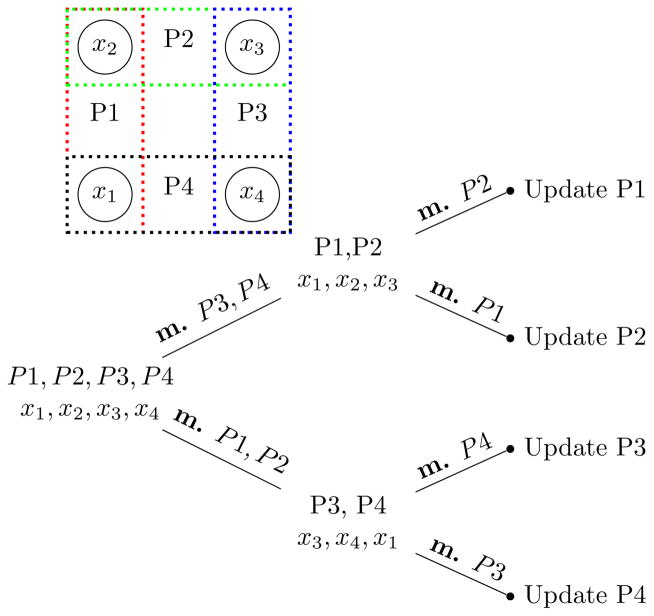
In fact, we can drastically speed up computations using a divide-and-conquer message passing scheme. This approach relies on the careful re-use of messages across pathway updates. Using such a scheme, we need to compute only O(k log k) messages per iteration. An example is shown in Figure 3. In the special case of pathways that form a tree structure, we can further improve this approach to compute only O(k) messages per iteration.

Figure 3.

Example with 4 pathways forming a cycle “m.” means marginalization.

4 Experiments

Since there is no learning algorithm designed to efficiently solve (2), we compared PathGLasso with the state-of-the-art learning algorithms for the graphical lasso problem (1) – QUIC (Hsieh et al. 2011) and HUGE (Zhao et al. 2012). Although neither of these competitors solves (2) directly, we adapt them to solve (2) by supplying a matrix of separate λ values for each entry in the inverse covariance matrix. We set λ = 10¹⁰ for the entries that lie outside of the pathways, making them solve exactly the same problem as Path-GLasso. We observed that supplying such a matrix improves performance of both methods due to the active set heuristics employed by these methods. Additionally, we compared with DP-GLASSO (Mazumder, Hastie, and others 2012), the method that we used to learn parameters in each pathway (8), to make sure that the superior performance of Path-GLasso is due to our decomposition approach as opposed to the use of DP-GLASSO. We note that DP-GLASSO is not competitive in this setting because it does not employ active set heuristics. All comparisons were run on 4 core Intel Core i7-3770 CPU @ 3.40GHz with 8GB of RAM.

4.1 Synthetic datasets comparison

We compared PathGLasso with QUIC, HUGE and DP-GLASSO on 3 scenarios: 1) Cycle: Pathways form one large cycle with 50 genes per pathway with overlap size of 10; 2) Lattice: The true underlying model is a 2D lattice, and each pathway contains between 3 and 7 nearby variables; and 3) Random: Each pathway consists of randomly selected genes. For each setting, we generated a true underlying connectivity graph, converted it to the precision matrix following the procedure from (Liu and Ihler 2011), and generated 100 samples from the multivariate Gaussian distribution.

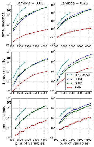
We observed that PathGLasso dramatically improves the run time compared to QUIC, HUGE and DP-GLASSO (Figure 4), sometimes up to two orders of magnitude. We note that DP-GLASSO, used as an internal solver for Path-GLasso, performs much worse than both HUGE and QUIC. This is because DP-GLASSO is not as efficient as QUIC or HUGE when solving very sparse problems due to the lack of active set heuristics. This is not a problem for Path-GLasso, because our within-pathway networks are small, and are much denser on average than the entire network.

Figure 4.

Run time (y-axis) for (A) Cycle, (B) Lattice and (C) Random (see text for details).

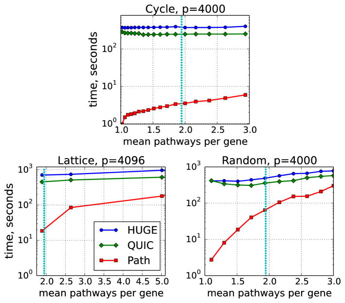
In addition to varying the number of variables p (Figure 4), we also explored the effect of the degrees of overlap among the pathways (Figure 5). We denote by η the sum of sizes of all pathways divided by the total number of variables in the entire network. This can be interpreted as the average number of pathways to which each variable belongs. In a non-overlapping model, η = 1. The parameter η grows with the size of the overlap between pathways. A set of pathways from a real biological database, called Reactome (Croft et al. 2011), has η = 1.95 (see Section 4.2).

Figure 5.

Run time for various values of η, with λ = 0.1. η = 1.95 is drawn as a dotted vertical line.

4.2 Real data experiments

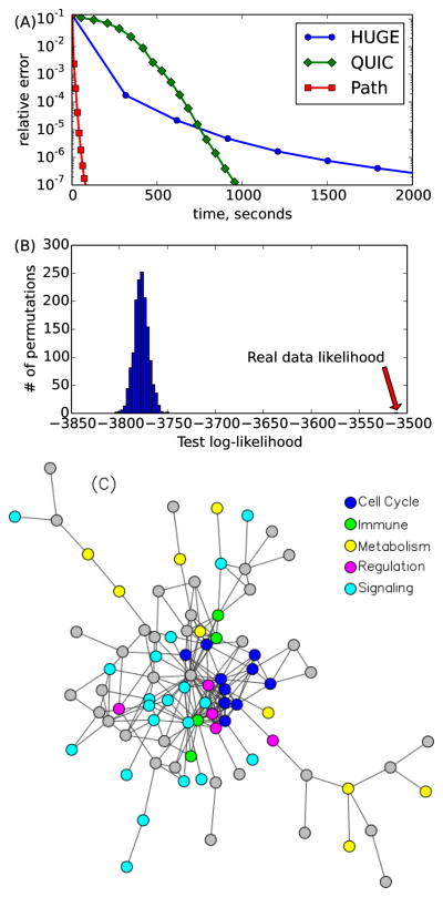
We considered two gene expression datasets from acute myeloid leukemia (AML) studies: MILE (Haferlach et al. 2010) and GENTLES (Gentles et al. 2010) containing 541 and 248 samples, respectively. The raw data were processed using the Affy R package, MAS5 normalized, and corrected for batch effects by ComBat. We used a widely used curated pathway database, called Reactome, that contains a set of genes for each biological pathway. We considered pathways containing fewer than 150 genes, which results in 4591 genes in 156 pathways. Large pathways are often supersets of smaller pathways; therefore, this filtering scheme allowed us to focus on finer-grained pathways. Following (Hsieh et al. 2011), we plotted the relative error (y-axis) against time (x-axis) in Figure 6A. We computed the relative error in the following way. All 3 methods (QUIC, HUGE and Path-GLasso) were run for an extended period of time with small tolerance parameters. We denote by Θ^* the learned parameter that leads to the lowest value of objective function. Relative error was then computed as |ll(Θ) − ll(Θ^*)|/|ll(Θ^*)|, where ll means the log-likelihood. Again, PathGLasso is significantly faster than HUGE and QUIC in the full range of relative errors. This experiment indicates that the choice of stopping criterion did not affect our results.

Figure 6.

MILE data (p = 4591, k = 156). (A) Relative error vs time, (B) Test log-likelihood on Gentles dataset for random pathways, (C) Significant pathway interactions.

5 Interpretation of the Learned Network

We first checked whether the constraints imposed by the Reactome pathways improved the generalization performance of the learned network. We computed the test log-likelihood of the network trained on the MILE data and tested on the GENTLES data. We compared the result with random pathways created by shuffling genes among the pathways, preserving the pathway sizes and the structure among the pathways. We observed that the test log-likelihood of the original Reactome pathways is significantly higher than those of random pathways (Figure 6B). This result indicates that the Reactome pathways capture relevant information about the underlying network structure among genes conserved in two independent datasets.

We will now show that PathGLasso provides a new way of interpreting the learned network. We identified pairs of pathways that have significant dependencies, by computing the sum of the magnitude of the edge weights that connect them, and comparing that with the quantity obtained from simulated 1500 data sets. Figure 6C shows a graphical representation of the dependencies among pathways. Interestingly, all of the cell cycle-related pathways are tightly connected with each other. Cancer is characterized by uncontrolled growth of cells, which is caused by deregulation of cell cycle processes (Collins, Jacks, and Pavletich 1997). One of the most densely-connected pathways is the “Cell Cycle Check Points” pathway, which is known to play a role in the central process of cancer progression by tightly interacting with many other pathways involved in the immune system, metabolism, and signaling (Collins, Jacks, and Pavletich 1997).

6 Conclusion

We introduced the pathway-constrained sparse inverse covariance estimation problem and a novel learning algorithm, called PathGLasso. We showed that our algorithm can be orders of magnitude faster than state-of-the-art competitors. We demonstrated that PathGLasso can leverage prior knowledge from curated biological pathways. PathGLasso uses an off-the-shelf algorithm for solving a standard graphical lasso problem as a subroutine, thus it will benefit from future performance improvements in the graphical lasso algorithms.

References

- Ambroise C, Chiquet J, Matias C. Inferring sparse gaussian graphical models with latent structure. Electronic Journal of Statistics. 2009;3:205–238. [Google Scholar]
- Banerjee O, El Ghaoui L, d’Aspremont A. Model selection through sparse maximum likelihood estimation for multivariate Gaussian or binary data. JMLR. 2008;9:485–516. [Google Scholar]
- Celik S, Logsdon B, Lee S-I. Efficient dimensionality reduction for high-dimensional network estimation. International Conference on Machine Learning (ICML).2014. [Google Scholar]
- Collins K, Jacks T, Pavletich NP. The cell cycle and cancer. Proceedings of the National Academy of Sciences. 1997;94(7):2776–2778. doi: 10.1073/pnas.94.7.2776. [DOI] [PMC free article] [PubMed] [Google Scholar]
- Croft D, OKelly G, Wu G, Haw R, Gillespie M, Matthews L, Caudy M, Garapati P, Gopinath G, Jassal B, Jupe S, Kalatskaya I, Mahajan S, May B, Ndegwa N, Schmidt E, Shamovsky V, Yung C, Birney E, Hermjakob H, DEustachio P, Stein L. Reactome: a database of reactions, pathways and biological processes. Nucleic Acids Research. 2011;39(suppl 1):D691–D697. doi: 10.1093/nar/gkq1018. [DOI] [PMC free article] [PubMed] [Google Scholar]
- Felleman DJ, Van Essen DC. Distributed hierarchical processing in the primate cerebral cortex. Cerebral cortex (New York, NY: 1991) 1991;1(1):1–47. doi: 10.1093/cercor/1.1.1-a. [DOI] [PubMed] [Google Scholar]
- Friedman J, Hastie T, Tibshirani R. Sparse inverse covariance estimation with the graphical lasso. Biostatistics. 2007;9:432–441. doi: 10.1093/biostatistics/kxm045. [DOI] [PMC free article] [PubMed] [Google Scholar]
- Gentles A, Plevritis S, Majeti R, Alizadeh A. Association of a leukemic stem cell gene expression signature with clinical outcomes in acute myeloid leukemia. JAMA. 2010;304(24):2706–2715. doi: 10.1001/jama.2010.1862. [DOI] [PMC free article] [PubMed] [Google Scholar]
- Haferlach T, Kohlmann A, Wieczorek L, Basso G, Kronnie G, Béné M, De Vos J, Hernández J, Hofmann W, Mills K, et al. Clinical utility of microarray-based gene expression profiling in the diagnosis and sub-classification of leukemia: report from the international microarray innovations in leukemia study group. Journal of clinical oncology: official journal of the American Society of Clinical Oncology. 2010;28(15):2529. doi: 10.1200/JCO.2009.23.4732. [DOI] [PMC free article] [PubMed] [Google Scholar]
- Honorio J, Samaras D, Paragios N, Goldstein R, Ortiz LE. Sparse and locally constant gaussian graphical models. In: Bengio Y, Schuurmans D, Lafferty J, Williams C, Culotta A, editors. Advances in Neural Information Processing Systems. Vol. 22. Curran Associates, Inc; 2009. pp. 745–753. [Google Scholar]
- Hsieh C-J, Sustik MA, Dhillon IS, Ravikumar P. Shawe-Taylor J, Zemel R, Bartlett P, Pereira F, Weinberger K, editors. Sparse inverse covariance matrix estimation using quadratic approximation. Advances in Neural Information Processing Systems. 2011. pp. 2330–2338. http://nips.cc/
- Hsieh C-J, Dhillon IS, Ravikumar P, Banerjee A. NIPS. 2012. A divide-and-conquer procedure for sparse inverse covariance estimation. [Google Scholar]
- Lauritzen S. Graphical Models. Oxford Science Publications; 1996. [Google Scholar]
- Liu Q, Ihler AT. Learning scale free networks by reweighted l1 regularization. AISTATS. 2011:40–48. [Google Scholar]
- Mardia K, Kent J, Bibby J. Multivariate Analysis. Academic Press; 1979. [Google Scholar]
- Mazumder R, Hastie T, et al. The graphical lasso: New insights and alternatives. Electronic Journal of Statistics. 2012;6:2125–2149. doi: 10.1214/12-EJS740. [DOI] [PMC free article] [PubMed] [Google Scholar]
- Meng Z, Wei D, Wiesel A, Hero A., III Distributed learning of gaussian graphical models via marginal likelihoods. JMLR. 2013;31:3947. [Google Scholar]
- Mizrahi YD, Denil M, de Freitas N. Linear and parallel learning for markov random fields. International Conference on Machine Learning (ICML).2014. [Google Scholar]
- Tseng P. Convergence of a block coordinate descent method for nondifferentiable minimization. Journal of optimization theory and applications. 2001;109(3):475–494. [Google Scholar]
- Wiesel A, Hero AO. Distributed covariance estimation in gaussian graphical models. Signal Processing, IEEE Transactions on. 2012;60(1):211–220. [Google Scholar]
- Yuan M, Lin Y. Model selection and estimation in the Gaussian graphical model. Biometrika. 2007;94(10):19–35. [Google Scholar]
- Zhao T, Liu H, Roeder K, Lafferty J, Wasserman L. The huge package for high-dimensional undirected graph estimation in r. J Mach Learn Res. 2012;13:1059–1062. [PMC free article] [PubMed] [Google Scholar]