Convex weighting criteria for speaking rate estimation

Abstract

Speaking rate estimation directly from the speech waveform is a long-standing problem in speech signal processing. In this paper, we pose the speaking rate estimation problem as that of estimating a temporal density function whose integral over a given interval yields the speaking rate within that interval. In contrast to many existing methods, we avoid the more difficult task of detecting individual phonemes within the speech signal and we avoid heuristics such as thresholding the temporal envelope to estimate the number of vowels. Rather, the proposed method aims to learn an optimal weighting function that can be directly applied to time-frequency features in a speech signal to yield a temporal density function. We propose two convex cost functions for learning the weighting functions and an adaptation strategy to customize the approach to a particular speaker using minimal training. The algorithms are evaluated on the TIMIT corpus, on a dysarthric speech corpus, and on the ICSI Switchboard spontaneous speech corpus. Results show that the proposed methods outperform three competing methods on both healthy and dysarthric speech. In addition, for spontaneous speech rate estimation, the result show a high correlation between the estimated speaking rate and ground truth values.

I. Introduction

Speaking rate (SR) is an important quantity in a number of applications in speech processing [1], [2], [3], [4], [5], [6], [7], [8], [9]. Speaking rate plays a critical role in automatic speech recognition (ASR) engines since it greatly impacts performance; it is well known that ASR error rates increase for unusually fast or unusually slow speech [7]. This has led to approaches that integrate online speaking rate estimation within the ASR engine and modify the recognition algorithms accordingly [1]. As a result, accurate online speaking rate estimation is a critical component in these applications.

In the context of speech motor control, speaking rate can be considered an index of the efficiency of articulatory movements over time [8], [9]. For this reason, abnormalities in speaking rate are common in disorders of motor speech, such as dysarthria, that arise from neurological disease or damage [9]. Weakness and/or incoordination among the muscles that subserve speech typically result in speech rate slowing as the patient attempts to achieve articulatory targets for the production of understandable speech. Automating speaking rate measures is challenged by the large variability of speech degradation patterns across individuals with neurological disease or injury [8]. Thus, an automated solution must be robust to degraded acoustic cues, and adaptable to the wide variety of speaking patterns.

Speaking rate is a critical component of successful discourse. In conversation it has been shown that speakers will modify their speaking rate so that it more closely matches their partner’s – a phenomenon known as entrainment [10], [11]. Speaking rate is also important in detecting prosodic prominence in conversations [12] and in reliably segmenting incoming speech [13]. As a result, a reliable and adaptable method for estimating speaking rate is an important part of a larger system for automatic discourse analysis.

A. Previous Work

Although there are many definitions for SR, the number of syllables per second is often preferred in the literature due to its high correlation with the perceptual SR [14]. Most of the previous work uses this definition and aims to estimate the number of syllables (or a related variant) from the speech waveform.

The original algorithms in the literature aiming to estimate speaking rate (see [14], [15], [16]) are derivations of the method in [17] for automatic detection of syllables in speech by detecting maxima in a loudness function. In more recent work in the area, Wang and Narayanan proposed to use subband spectral and temporal correlations with the aid of voicing information to detect syllables [18]. Jong and Wempe showed that a simple detector based on intensity and voicing can detect syllable nuclei [19]. Zhang and Glass estimate SR by fitting a sinusoid to the Hilbert envelope such that the peaks of the sinusoid coincide with the peaks of the envelope of the speech signal [20].

These methods follow a similar paradigm: extract acoustic features (e.g. subband energy, loudness, time-frequency correlations) in the first step, then develop a temporal envelope that is used to count peaks and valleys using different strategies. The number of peaks and their locations yield the potential vowel nuclei and the number of vowels is used as a proxy for the number of syllables. However, since spoken speech is widely variable, spurious peaks in the envelope are likely to show similar characteristics to the vowel peaks in the envelope. The existing algorithms aim to minimize the effects of additional peaks by using heuristics and defining new thresholds, making the resulting methods less robust to new data. In lieu of thresholding, other approaches involving statistical learning have appeared in the literature [21], [22]; however these approaches result in non-convex optimization criteria with high-dimensional unknown parameters, making training difficult and potentially unreliable.

The literature on speech segmentation is also relevant to the problem of SR estimation [23], [24], [25]. These algorithms aim to identify the nuclei and boundaries of different syllables given only the speech waveform. Although they are useful for identifying individual vowels or syllables, we note that to estimate SR, the precise locations of the vowels are not necessary. Indeed, it seems ill-advised to solve the more difficult problems of speech segmentation if our quantity of interest (speaking rate) only requires knowledge of the number of syllables in a given utterance and the length of the utterance.

Here we propose a more direct way of estimating the speaking rate that does not require segmentation, detection, or peak counting. Our approach is motivated by the work of counting objects in an image [26], in which the authors learn a linear transformation of an image feature representation that approximates the object density in a set of training images. In our work, we develop new convex criteria to learn an optimal weighting function for estimating the number of vowels in a given interval. We impose the constraint that when a time-frequency representation of a speech signal is projected on the learned weighting function the result is a temporal vowel density function. The integral of the temporal vowel density function over a given interval yields the number of vowels within that interval. We also define a speaker adaptation strategy to customize the weighting function for a given speaker, requiring only a single labeled sentence from that speaker (the label is the number of vowels in an utterance). This is especially useful in our experiments with dysarthric speech, where there exists significant deviation between the dysarthric speech used in testing and the healthy speech used to learn the weighting function. We compare the proposed approaches against three competing methods in the literature, [18], [19], [21] on two tasks: estimating the SR in the TIMIT corpus [27] and estimating SR on a dysarthric speech corpus [8]. The results show that the proposed methods consistently result in lower error rates. In addition, we also show the effectiveness of the proposed methodology in estimating speaking rate on a spontaneous speech corpus.

This paper is organized as follows. In section II, we introduce two convex cost functions for learning the weighting function and another for speaker adaptation. In section III, we describe the experimental setup and the results on the TIMIT corpus, a dysarthric speech corpus, and a spontaneous speech corpus. In section IV we make concluding remarks and describe future work.

II. Speaking Rate Estimation

As discussed in the previous section, most of the work in this area uses the number of syllables per second (or some variant) as an estimate of speaking rate. Each syllable consists of three components: the onset (a consonant), the nucleus (a sonorant, vowel), and the coda (a consonant). Since every syllable must contain a vowel, we reformulate the syllable counting problem as the closely related problem of counting the vowels in a speech segment. As a result, in the work we present here, we use the number of vowels per second as a proxy for the syllable rate.

Consider a speech signal, x_i(t), where i is the index of the speech sample, with sampling rate F_s and length T_i. We partition the signal into N_i frames of equal length and, for each frame, we extract a set of D features. We denote the resulting matrix by X_i ∈ R^Ni×D. The features can correspond to the magnitude spectrum of each frame, average energy value in a set of sub-bands, mel-frequency cepstral coefficients (MFCC), etc. For the majority of the experimental results in section III, we use subband log-energy features in order to compare against the results in [18]; however, as we will see later, one of the benefits of the proposed approach is that we are able to use different feature sets.

The goal of our approach is to determine an optimal weighting function for the features, w, such that the speaking rate of speech segment x_i(t) (denoted by SR_i) can be estimated through temporal integration of the weighted features,

$$S{R}_i=\frac{1}{T_i}{\displaystyle \sum _{k=1}^{N_i}{\displaystyle \sum _{j=1}^D{\mathbf{X}}_i(k,j)}\mathbf{w}(j)}.$$ (1)

With Eq. (1), our goal is to identify the number of vowels (not necessarily their location) in each utterance and to normalize by the corresponding duration of the utterance. In the ensuing sections, we define multiple optimization criteria for determining an optimal w. The assumption is that we will optimize over w using labeled data from an available training set and evaluate the resulting algorithm on speech from speakers outside of the training set.

A. Criterion 1: Optimization with individual vowel labels

For each utterance in our training set, we consider a sparse label vector, l_i(k), where k ∈ [1, 2, …, N_i] that is positive only for values of k that fall during the occurrence of a vowel and is zero otherwise. Furthermore, we scale this label vector to be a density function whose integral (in time) over the utterance yields the number of vowels in that utterance. Let us consider the speech sample in Fig. 1 where we show the speech waveform, spectrogram, and the corresponding label vector. The label vector is non-zero only during a vowel occurrence and, in that interval, the value of the label is inversely proportional to the duration of the vowel. For example, for the vowel “eh”, the start and end times are k₁ and k₂ respectively and the label vector has a value of $\frac{1}{k_2-k_1}$ during that interval. The label vector is defined in the same manner for all other vowels, ensuring that its integral yields the number of vowels contained in the speech segment (e.g. ${\displaystyle {\sum }_{k=1}^{N_i}{\mathbf{l}}_i(k)}=10$ for the example in Fig. 1).

Fig. 1.

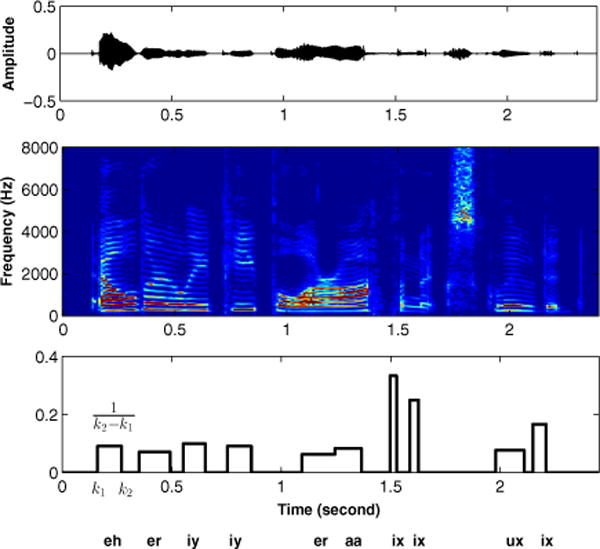
Top: The speech waveform of a sample utterance from the TIMIT corpus. Middle: The spectrogram of the same utterance. Bottom: The labeled vowel vector l(k) whose sum over an interval yields the number of vowels in that interval. For this sample, Σ_k l(k) = 10.

According to equation (1), the ideal weight vector, w, when projected on the feature matrix and summed in time yields the number of vowels. In other words, for any speech sample in our training set, the optimal w would ideally satisfy

$${\displaystyle \sum _{k=1}^{N_i}{\mathbf{l}}_i(k)}={\displaystyle \sum _{k=1}^{N_i}{\displaystyle \sum _{j=1}^D{\mathbf{X}}_i(k,j)}\mathbf{w}(j)}.$$

Furthermore, for any subset of the whole sentence, (e.g. for any interval $\left[k_i^{\text{start}},k_i^{\text{start}}+1,\dots ,k_i^{\text{end}}\right]\in [1,2,\dots ,N_i]$), the optimal w would ideally satisfy

$${\displaystyle \sum _{k=k_i^{\text{start}}}^{k_i^{\text{end}}}{\mathbf{l}}_i(k)}={\displaystyle \sum _{k=k_i^{\text{start}}}^{k_i^{\text{end}}}{\displaystyle \sum _{j=1}^D{\mathbf{X}}_i(k,j)}\mathbf{w}(j)}.$$ (2)

We propose a convex cost function to learn an optimal w based on these labels for all utterances in the training set. Let us consider a training set of size N^train. For every sentence i ∈ [1, …, N^train], we consider M random subsets, where for subset m ∈ [1 … M], the values of k fall in the interval $\left[k_{i,m}^{\text{start}},k_{i,m}^{\text{start}}+1,\dots ,k_{i,m}^{\text{end}}\right]$ – this is a sub-segment of the entire sentence, [1, 2, …, N_i]. In other words, we split each sentence into M random intervals and generate a set of constraints for our objective function. The equations resulting from the relationship in (2) (for all intervals in all utterances in the training set) are used to constrain the solution of the proposed objective function. Similar to the epsilon-insensitive loss in support vector regression [28], we introduce variables ξ_i,m, to bound the difference between the actual number of vowels and the predicted number of vowels in each interval from above and below as follows:

$$-{\xi }_{i,m}\le {\displaystyle \sum _{k=k_{i,m}^{\text{start}}}^{k_{i,m}^{\text{end}}}{\mathbf{l}}_i}(k)-{\displaystyle \sum _{j=1}^D{\mathbf{X}}_i}(k,j)\mathbf{w}(j)\le {\xi }_{i,m}.$$

In Algorithm 1 (OPT-Seg), we define a notional optimization problem that aims to minimize the sum of the ℓ₁-norm of w and the ℓ₂-norm of the variables ξ_i,m, where i ∈ [1 … N^train] and m ∈ [1 … M]. The 2MN^train inequality constraints outlined above and the D non-negativity constraints on w determine the region of feasibility for this convex objective function. This results in a sparse solution in w, where only a subset of the D features are selected in the summation. The sparsity criterion serves two purposes: First, since any acoustic features or their combination can be used, the sparsity criterion performs model selection by only using a subset of the features; Second, when the training samples are not sufficient relative to the dimension of features, the sparsity criterion acts as a regularizer in order to prevent overfitting.

Algorithm 1 OPT-Seg

$$\begin{array}{ll}\underset{\mathbf{w},{\xi }_{i,m}}{\text{minimize}}& {\Vert \mathbf{w}\Vert }_1+{\displaystyle \sum _{i=1}^{N^{\text{train}}}{\displaystyle \sum _{m=1}^M{\xi }_{i,m}^2}}\\ \text{subject to}& {\displaystyle \sum _{k=k_{i,m}^{\text{start}}}^{k_{i,m}^{\text{end}}}{\displaystyle \sum _{j=1}^D{\mathbf{X}}_i}(k,j)\mathbf{w}(j)-{\mathbf{l}}_i(k)\le {\xi }_{i,m}}\\ & {\displaystyle \sum _{k=k_{i,m}^{\text{start}}}^{k_{i,m}^{\text{end}}}{\mathbf{l}}_i}(k)-{\displaystyle \sum _{j=1}^D{\mathbf{X}}_i}(k,j)\mathbf{w}(j)\le {\xi }_{i,m}\\ & \mathbf{w}\ge 0\end{array}$$

It is clear that OPT-Seg requires careful labeling of each vowel in each utterance, as in Fig. 1, since we require knowledge of ${\displaystyle {\sum }_{k=k_{i,m}^{\text{start}}}^{k_{i,m}^{\text{end}}}{\mathbf{l}}_i}(k)$ for any interval m in utterance i. This may be costly and prohibitive in some circumstances. In the ensuing section, we modify the cost function such that only the number of vowels in each training sample are required to learn an optimal w.

B. Criterion 2: Optimization with vowel counts

A significantly easier task than careful labeling of all vowels in the speech signal is obtaining the number of vowels in each utterance, s_i. Using the notation in the previous section, for training utterance x_i(t), this corresponds to knowing $s_i={\displaystyle {\sum }_{k=1}^{N_i}{\mathbf{l}}_i}(k)$ rather than having knowledge of ${\displaystyle {\sum }_{k=k_{i,m}^{\text{start}}}^{k_{i,m}^{\text{end}}}{\mathbf{l}}_i}(k)$ for all i ∈ [1 … N^train], m ∈ [1 … M].

In this formulation, we remove the random sub-sampling required in OPT-Seg and change the region of feasibility of the optimization problem to include only constraints corresponding to each training utterance. The resulting optimization problem is shown in Algorithm 2 (OPT-Sent). As with the OPT-Seg, we still minimize the sum of the ℓ₁-norm of w and the ℓ₂-norm of the variables ξ_i; however the constraint set defines a different region of feasibility. For the same number of training samples, removing the random sub-sampling of each utterance results in far fewer variables and constraints than the algorithm in OPT-Seg. The number of constraints in OPT-sent is 2N^train + D and the dimension of unknown variable is N^train + D (instead of the 2MN^train + D constraints and MN^train + D variables in OPT-Seg).

Algorithm 2 OPT-Sent

$$\begin{array}{ll}\underset{\mathbf{w},{\xi }_i}{\text{minimize}}& {\Vert \mathbf{w}\Vert }_1+{\displaystyle \sum _{i=1}^{N^{\text{train}}}{\xi }_i^2}\\ \text{subject to}& {\displaystyle \sum _{k=1}^{N_i}{\displaystyle \sum _{j=1}^D{\mathbf{X}}_i}(k,j)\mathbf{w}(j)-s_i\le {\xi }_i}\\ & s_i-{\displaystyle \sum _{k=1}^{N_i}{\displaystyle \sum _{j=1}^D{\mathbf{X}}_i}(k,j)\mathbf{w}(j)\le {\xi }_i}\\ & \mathbf{w}\ge 0\end{array}$$

C. Criterion 3: Speaker-specific adaptation

For both of the optimization criteria, the assumption is that the weighting function is trained on multiple speech samples from different speakers. For out-of-sample speakers, particularly those with atypical speech production (e.g. dysarthric speakers), the resulting weighting functions would likely need further adaptation. Here we propose a speaker adaptation strategy to further customize the weighting vector to a particular speaker. We assume that we have a single utterance from the test speaker, x_a(t), for which we know the number of vowels, s_a.

We define a new weighting vector, w′ = Tw, where T is set to be a tridiagonal weighting matrix with positive real numbers on its diagonal and off-diagonal positions and zeros otherwise. This models the values of a particular component of w′ as a linear combination of neighboring components in w. Specifically, the n^th component of w′ can be written as

$$\mathbf{w}\prime (n)={\displaystyle \sum _{i=-1}^1\mathbf{T}(n,n+i)}\mathbf{w}(n+i),$$ (3)

where any values of T(n, n + i) or w(n + i) for n + i < 0 or n + 1 > D are defined as zero.

The motivation for the tridiagonal matrix is clear for frequency domain features. As we will see in the ensuing section, the learned vector w highlights frequency features related to pitch and formants. By only locally adapting, the position and amplitudes of the weights can be adjusted according to the differences of individuals’ pitch and formant frequencies and energies. In Algorithm 3, we define new optimization criteria that can be used to learn T from a single labeled sentence. The solution to Algorithm 3 yields a new weighting function w′ = Tw which is unique to the target speaker. Thus the speaking rate can be estimated with Equation (1) by replacing w(j) with w′(j). Note that the tridiagonal constraint only makes sense for speech features that have significant overlap between adjacent channels, however, it may not be appropriate for features that are somewhat decorrelated between channels (e.g. MFCCs, combinations of different feature sets). In this case, the tridiagonal matrix can be replaced with a diagonal matrix.

On one hand, our aim is to refine the existing solution rather than to generate a new weighting vector. As a result, the cost function penalizes solutions of T that deviate from the identity matrix – this ensures that the w′ is not significantly different from w. On the other hand, we want the adapted weighting function to model the test speaker’s characteristics. As a result, the new region of feasibility only contains the single constraint from the labeled test sentence and the non-negativity criteria on T. We denote this algorithm by OPT-Seg-Adap if used to refine the solution of Algorithm 1 and by OPT-Sent-Adap if used to refine the solution of Algorithm 2.

Algorithm 3 Speaker adaptation

$$\begin{array}{ll}\underset{\mathbf{T}}{\text{minimize}}& {\Vert \mathbf{T}-1\Vert }_2\\ \text{subject to}& {\displaystyle \sum _{k=1}^{N_a}{\displaystyle \sum _{j=1}^D{\mathbf{X}}_a}(k,j)\mathbf{t}(j)\mathbf{w}(j)=s_a}\\ & \mathbf{T}\ge 0\\ & \mathbf{T}(i,j)=0,\forall j>i+1;1\le i,j\le D\\ & \mathbf{T}(i,j)=0,\forall j>i-1;1\le i,j\le D\end{array}$$

D. Solving the optimization problems

Since all three cost functions are convex, CVX, a Matlab-based modeling system for convex optimization, is used [29] [30]. Here we use the SeDuMi solver (packaged with CVX); this is a solver for solving optimization problems over symmetric cones [31]. We used the default precision settings in CVX ( cvx_precision = default) and no SeDuMi settings were changed from their default values.

III. Experiments and Results

We present experimental results on three data sets: the TIMIT database [27], a dysarthric speech database [8], and the ICSI Switchboard corpus [32]. We compare the proposed algorithms to three state-of-the-art approaches.

A. Evaluation on the TIMIT speech database

1) Extracting the features and training the model

TIMIT is a phonetically rich and balanced speech corpus that contains 630 speakers of eight major dialects of American English [27]. For each speaker, the database has spoken sentences sampled at 16-bit, 16kHz and labeled at the phoneme level. Approximately 73% of speech samples (462 speakers, 4620 sentences) were assigned to the training set and the remaining (168 speakers, 1680 sentences) were reserved for testing.

The speech samples were analyzed using a 20 ms Hamming window with a 10 ms frame shift. Subband log-energy features were extracted for each frame using a 19-channel Butterworth filterbank [33]. In other words, 19 log-energy coefficients (one per sub-band) were computed for each 20 ms frame – we denote this feature vector by $\stackrel{\sim }{\mathbf{X}}$. For each frame k, we further normalize the feature vector as follows

$$\mathbf{X}(k,j)=\frac{\stackrel{\sim }{\mathbf{X}}(k,j)-{\min }_j(\stackrel{\sim }{\mathbf{X}}(k,j))}{{\max }_j(\stackrel{\sim }{\mathbf{X}}(k,j))-{\min }_j(\stackrel{\sim }{\mathbf{X}}(k,j))}.$$

The normalization is based on each frame, and the ${\min }_j(\stackrel{\sim }{\mathbf{X}}(k,j))$ and ${\max }_j(\stackrel{\sim }{\mathbf{X}}(k,j))$ represent the minimum and maximum values of the D dimensional features for frame k. This results in a feature set normalized between 0 and 1 for every frame. The purpose of normalization is to bring the intensity of every vowel to the same level because all frames in each channel share the same weights in the weighting factor. One of the disadvantages of such normalization is that it may also bring the speech segments with very low energy, such as silence and some fricatives to the same intensity level as the vowels. An alternative approach could be to do the normalization within a short interval instead of on each frame. Empirically, we did not see any difference in performance between the two approaches therefore we use the frame-based normalization strategy.

The sparse label vectors for the TIMIT data were generated with a single value for each frame using the phoneme labels contained in TIMIT (see the sparse label in Fig. 1 (Bottom)). For evaluation, we solve the optimization problems in OPT-Seg and OPT-Sent and their counterparts with adaptation. For OPT-Seg, the number of random speech segments in each sentence was set to M = 20. The solution to the optimization problems was obtained using the CVX toolbox in Matlab.

2) Evaluating the model

In the evaluation stage, we tested the two weighting functions from OPT-Seg and OPT-Sent on the TIMIT test data and then used our proposed speaker adaptation strategy to test again. For OPT-Seg and OPT-Sent, two weighting functions learned respectively from the TIMIT training data were used on all test speakers without modification. For OPT-Seg-Adapt and OPT-Sent-Adapt, a single randomly selected sentence from each speaker in the test set was used to modify the original weighting vectors obtained in OPT-Seg and OPT-Sent, which meant each speaker has a unique model to evaluate on his/her remaining speech samples. In Fig. 2, we show a sample utterance from the test set. The figure shows the speech waveform, the resulting spectrogram, the learned weighting functions using OPT-Sent and OPT-Sent-Adap, and the projection of the features for this utterance on the weighting functions – the temporal vowel density function. From the figure, we can see that the optimal weighting functions highlight important components in frequency bins likely related to the first two formants. Adaptation results in a small change in the learned weighting function compared to the original and provides a better fit for this particular test speaker. The speaking rate can be estimated by temporal integration of the vowel density function, normalized by the time interval.

Fig. 2.

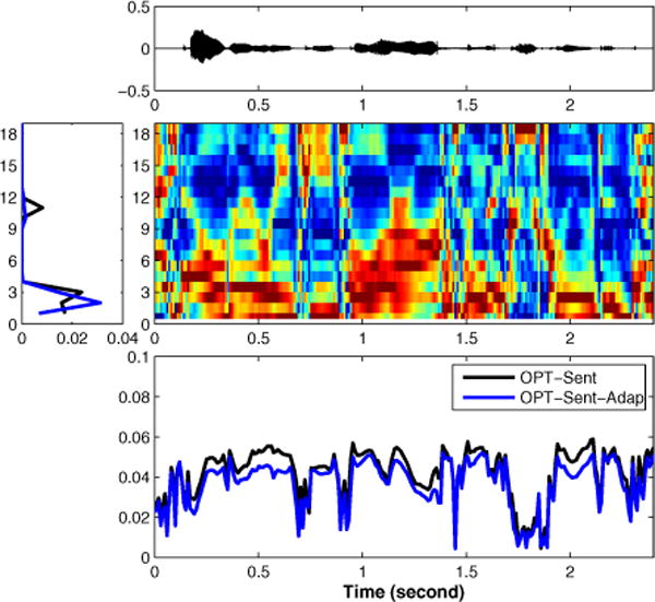
Top: The speech waveform of a sample utterance from the TIMIT test corpus. Middle Right: The normalized log-energy features extracted by the 19-channel Butterworth filterbank. Middle Left: The optimal weighting function before and after adaptation. Bottom: The temporal vowel density function before and after adaptation.

It is important to note that the temporal vowel density function (Fig. 2 (Bottom)) looks distinctly different from the sparse label vector (Fig. 1 (Bottom)). This is expected since the goal of the optimization criteria is not to learn this sparse label vector directly. Rather, the integral of both waveforms between two time points should yield a similar value. In Fig. 3, we plot the vowel density functions of a test sentence using the w vector from OPT-Sent and OPT-Sent-Adap (Top) and the vowel label (Middle). Although they look different, their integral between 0 and time t match up quite well (see Fig. 3 (Bottom)). This is especially true for the adapted weight vector.

Fig. 3.

Top: The temporal vowel density function before and after adaptation for a TIMIT test sentence. Middle: The sparse labeling function for this sentence. Bottom: The integral of the density functions (before and after adaptation) and the sparse labeling function from 0 to t.

We compared our results with three state-of-the-art methods: the Intensity-based Praat script method (Inten-Praat) [19], the time/frequency correlation-based method (TF-Corr) [18], and the GMM-neural network based method (GMM-NN) [21]. For Inten-Praat, we implemented the Praat script directly on the TIMIT testing speech since this method did not require any training or parameter tuning. For TF-Corr and GMM-NN, we used the same TIMIT training data to select a set of optimal parameters for TF-Corr and to train the model for GMM-NN. We then evaluated both algorithms on the same TIMIT testing data. The TF-Corr algorithm was trained using the Monte-Carlo procedure suggested in [18]. The GMM-NN algorithm was trained using a combination of the maximum likelihood algorithm and back-propagation [21]. The results are shown in Table I. We use four metrics in the evaluation: the correlation coefficient between the predicted and the actual number of vowels in the test sentences; the average vowel count error, computed as the absolute error of the number of vowels in each test sentence, averaged over all data in the test set, and its standard deviation; the SR error rate, computed as the average of $\frac{\left|\text{predicted}-\text{actual}\right|}{\text{actual}}$ across all sentences in the test set; the SR mean error, computed as the absolute error between the true speaking rate and the predicted speaking rate in each test sentence, averaged over all data in the test set, and its standard deviation.

TABLE I.

Comparative results on the TIMIT corpus

Method	Corr coeff	Mean error	Stddev error	SR error rate%	SR mean error	SR stddev error
Inten-Praat	0.890	1.93	1.38	15.4	0.639	0.49
TF-Corr	0.830	1.82	1.48	15.0	0.610	0.40
GMM-NN	0.805	1.61	1.41	14.0	0.528	0.41
OPT-Seg	0.842	1.57	1.25	13.7	0.498	0.39
OPT-Seg-Adap	0.869	1.39	1.24	12.2	0.462	0.36
OPT-Sent	0.841	1.58	1.34	13.9	0.514	0.40
OPT-Sent-Adap	0.867	1.40	1.24	12.4	0.464	0.37

From the results, it is clear that the proposed methods result in lower error rates and lower mean errors when compared to the three competing methods. We use a t-test to determine whether the differences between the results from our algorithms and the existing approaches are statistically significant. The resulting p-values are all very close to 0, meaning the improvement is statistically significant. These results are further improved when using speaker-specific weighting functions¹. Furthermore, OPT-Sent compares favorably to OPT-Seg, meaning that even if phoneme labels are not available, we can still train a reliable weighting function by knowing the total number of syllables in each sentence. The Inten-Praat results are interesting – this method yields a higher correlation coefficient, however it also has the largest mean error of all the methods. This means that the method captures the general trend, however it has a relatively large bias, which means it tends to either over- or under-estimate the exact number of syllables in each utterance.

3) Error analysis

From the results in Table I, we can see that the performance of OPT-Seg and OPT-Sent are similar. Although OPT-Seg requires careful vowel labels while OPT-Sent does not, their objectives are the same – ensure that the sum of the vowel density function approximates the number of vowels in a certain interval. The difference is that in OPT-Seg, such intervals are randomly cut from the training sentence, while in OPT-Sent, the whole sentence is used as the interval. Our results show that when a large sample size is used to train both algorithms (N^train = 4620 sentences), the results are similar. This implies that there are diminishing returns from adding additional constraints to the cost function generated from random splitting of the training sequences. Here we further investigate the effects of a varying sample size on algorithm performance.

Figure 4 (Top) shows the results of the four proposed algorithms trained on a smaller data set. The training data was randomly selected from TIMIT training data and the number of random segments in each sentence for OPT-Seg was set to 100 (M = 100). The evaluation results are based on all of the test data. For the OPT-Seg algorithms (with and without adaptation), we can see that performance asymptotes after fewer training sentences. This is due to the additional constraints in the cost function generated through the random sub sampling of the training sentences. The OPT-Sent algorithms require additional training data; even so, when the sample size reaches 500 sentences (N^train = 500), the performance of the OPT-Sent methods is comparable to the OPT-Seg algorithms (see Fig. 4 (Bottom)). This implies that to train the optimal weighting function in this example, we can either use 500 speech samples, knowing only the number of vowels in each utterance; or we can use fewer speech samples with carefully annotated vowel labels.

Fig. 4.

Top: A comparison of convergence characteristics of the four algorithms as a function of training set size. M = 100 for OPT-Seg and OPT-Seg-Adap. Bottom: A comparison of the convergence characteristics of OPT-Sent and OPT-Sent-Adap for larger training sets. X-axis is shown in log scale.

4) Evaluation on different features

The dimension of the acoustic feature set (D) is another consideration when analyzing the performance of the algorithm. In the above experiments, the time-frequency features were extracted by a 19-channel Butterworth filterbank in order to compare against the algorithm in TF-Corr that makes use of the same feature set.

We now vary the number of channels in the Butterworth filter and analyze the performance of the algorithm as a function of feature order. We use the frequency mapping proposed in [33] and resample the mapping for different filter orders. The results in Table II show that the higher order features tend to result in lower performance. The maximal performance is achieved for the 13-channel Butterworth filter, however there is no significant difference between 13-order and 7-order features (p = 0.596). These results are consistent with those in [34], showing that, for speaking rate estimation, a lower dimensional feature order is preferred. The reason for this could be that, for speaking rate estimation, larger bandwidths improve the generalization of the learning algorithm.

TABLE II.

The effect of feature dimension on performance

Order of features	Corr coef	Mean error	SR error rate%	SR mean error
7	0.869	1.39	12.1	0.476
13	0.871	1.39	12.0	0.462
19	0.867	1.40	12.4	0.464
32	0.865	1.41	12.6	0.465
64	0.858	1.49	13.3	0.480

With existing methods for estimating the speaking rate, the features cannot be decoupled from the estimation algorithm itself. One of the benefits of the proposed approach is that different feature sets can be used. In our experiment in Table I, we used 19-order Butterworth features, but the algorithm can be adapted to work on any acoustic feature set provided that the weighting function is trained and tested on the same feature type. Here we compare the performance of Butterworth filterbank features (ButtW) with three other feature sets: Mel frequency cepstrum coefficient (MFCC) [35], cochleagram features (Coch) [36] and Mel-spectrum with cubic root compression features (MelRoot3) [37]. We set the order of each feature set to 13 since that yields maximum performance for the ButtW features. We set T to be tridiagonal for ButtW, Coch, and MelRoot3 and diagonal for MFCC. The results are shown in Table III. The results indicate that the proposed method yields good performance on different feature sets. In fact, the MelRoot3 features slightly outperform the ButtW features, indicating that further improvements in performance are possible by analyzing different feature sets.

TABLE III.

The effect of feature type on performance

Features	Corr coeff	Mean error	SR error rate%	SR mean error
ButtW	0.871	1.39	12.0	0.462
MFCC	0.854	1.46	12.7	0.491
Coch	0.859	1.50	13.5	0.608
MelRoot3	0.881	1.33	11.4	0.454

B. Evaluation on a dysarthric speech database

For this experiment we made use of a dataset collected in the Motor Speech Disorders Laboratory at Arizona State University, consisting of 57 dysarthric speakers. Dysarthria is a motor speech disorder resulting from impaired movement of the articulators used for speech production; it is a condition secondary to an underlying neurogenic disorder. The dysarthria speakers include: 16 speakers with ataxic dysarthria, secondary to cerebellar degeneration, 15 mixed flaccid-spastic dysarthria, secondary to amyotrophic lateral sclerosis (ALS), 20 speakers with hypokinetic dysarthria, secondary to idiopathic Parkin-sons disease (PD), and 5 speakers with hyperkinetic dysarthria, secondary to Huntingtons disease (HD). Each speaker provided 5 spoken sentences, resulting in a total of 285 sentences across all speakers. The sentences for each speaker were:

• The supermarket chain shut down because of poor management

• Much more money must be donated to make this department succeed

• In this famous coffee shop they serve the best doughnuts in town

• The chairman decided to pave over the shopping center garden

• The standards committee met this afternoon in an open meeting

The details of the data collection strategy can be found in [8].

A description of the cardinal perceptual symptoms present in the different dysarthrias can be found in Table IV. As is apparent from the table, dysarthric speech exhibits greater variability when compared to healthy speech, therefore estimating speaking rate for dysarthric speech is much more challenging. The weighting function was trained on the TIMIT corpus with OPT-Sent. The tridiagonal transformation matrix was learned using a single labeled exemplar from each speaker – the remaining four exemplars for each speaker were reserved for testing. In Fig. 5, we show four sample waveforms from four individuals and the corresponding weighting functions before and after adaptation. In all figures, there is a significant difference between the weights before and after adaptation. This is expected since the original weights are learned using healthy speech from the TIMIT database and, as we see in Table IV, there is a significant difference between dysarthric speech and healthy speech. For Ataxic and ALS speech, the average value of the projected waveform decreases after adaptation. This is expected given the slow articulation rate that is associated with the speakers. For HD speech, there seem to be more fine-grained differences between the projected waveforms before and after adaptation. This is consistent with the irregular rate changes associated with HD. For PD speech, we see that the value of the projected waveform increases after adaptation. This is to account for the rapid articulation rate associated with PD speech.

TABLE IV.

Differences in perceptual symptoms present in different dysarthria subtypes

Ataxic	Scanning speech; imprecise articulation with irregular articulatory breakdown; irregular pitch and loudness changes
ALS	Prolonged syllables; slow articulation rate, imprecise articulation; hypernasality; strained strangled vocal quality
HD	Irregular pitch and loudness changes; irregular rate changes across syllable strings
PD	Rapid articulation rate; rushes of speech; imprecise articulation; monopitch; reduced loudness; breathy voice

Fig. 5.

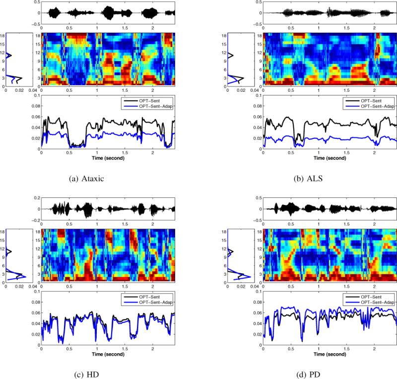
Examples of the optimal weighting functions (before and after adaptation) applied to 4 test utterances from the different dysarthria subtypes: (a) Ataxic, (b) ALS, (c) HD, and (d) PD. For each figure: Top: The speech waveform of a sample utterance from the four dysarthria subtypes. Middle Right: The normalized log-energy features extracted by the 19-channel Butterworth filterbank. Middle Left: The optimal weighting functions before and after adaptation. Bottom: The temporal vowel density functions before and after adaptation.

We compared the proposed approach with the Inten-Praat, TF-Corr and GMM-NN methods. The Inten-Praat method was directly implemented. As was done with our approach, for the TF-Corr method, we used one sentence from each speaker to select a best set of parameters and then tested on the remaining sentences. For the GMM-NN method, we trained four models (one for each dysarthria subtype) by using one sentence from each speaker and tested on other sentences. The results are shown in Table V. The five sentences used in the evaluation had approximately the same number of syllables each (between 15 and 17). As a result, estimating reliable correlation coefficients becomes difficult with a small sample size. We therefore focus on the average vowel count error, SR error rate and mean SR error. The table shows that our proposed speaker adaptation strategy outperforms the other three method significantly. This is expected since the adaptation significantly changes the optimal weighting vector, making it more suitable for the particular speaker.

TABLE V.

Comparative results on the dysarthric speech corpus

Method	Measure	Ataxic	ALS	HD	PD
Inten-Praat	SR error rate%	13.1	21.1	17.4	20.3
	SR mean error	0.35	0.41	0.50	1.06
	Mean error	2.21	3.32	2.76	3.30
TF-Corr	SR error rate%	15.7	25.2	19.7	16.8
	SR mean error	0.55	0.54	0.59	0.74
	Mean error	2.56	4.09	3.2	2.75
GMM-NN	SR error rate%	12.1	13.4	22.8	21.3
	SR mean error	0.31	0.31	0.65	1.07
	Mean error	2.10	2.20	3.87	3.48
OPT-Sent-Adap	SR error rate%	7.0	7.6	13.2	12.8
	SR mean error	0.23	0.21	0.42	0.69
	Mean error	1.20	1.30	2.26	2.12

C. Spontaneous speech rate estimation

Changes in speaking rate occur when the number and duration of pauses in the utterance is changed and the time spent on articulation is modified [38]. These two phenomenons are particularly prominent in spontaneous speech. Thus, estimating speaking rate on spontaneous speech is more challenging than that on read speech. To examine the performance of the proposed method on spontaneous speech, we evaluated it on the ICSI Switchboard corpus subset with phonetic transcription. In the dataset, there are 5564 speech samples segmented from the Switchboard corpus which includes several hundred informal speech dialogs recorded over the telephone [32]. Each speech sample has a hand labeled transcription, including syllable boundary information.

These rapid variations in speaking rate make estimation difficult. The algorithms we proposed extract features at each 20 ms frame. For rapid changes in SR, we find that frame-level features do not adequately capture these variations. To solve this problem, we use statistical features extracted at the sentence level which correlate with changes in speaking rate and we modify OPT-Sent so that it directly estimates the syllable rate instead of the number of syllables. The statistical features were calculated from a combination of several acoustic features, including the aforementioned Butterworth features (13 features), MFCC and its delta and delta-delta (39 features), cochleagram features (32 features), and MelRoot3 and its delta and delta-delta (39 features). The mean value and standard deviation of each channel of the features were calculated at the sentence level. Moreover, we also included the envelope modulation spectrum (EMS) feature set (60 features), known to be a useful indicator of atypical rhythm patterns in pathological speech [39]. They are concatenated as a 306-dimension vector of statistical features for each speech sample, ${\mathbf{X}}_i^{\text{sta}}$. To account for the fact that these are no longer frame-level features, we modify OPT-Sent as follows:

$$\begin{array}{ll}\underset{{\mathbf{w}}_s,{\xi }_i}{\text{minimize}}& {\Vert {\mathbf{w}}_s\Vert }_1+\lambda {\displaystyle \sum _{i=1}^{N^{\text{train}}}{\xi }_i^2}\\ \text{subject to}& {\mathbf{X}}_i^{\mathit{sta}}{\mathbf{w}}_s-r_i\le {\xi }_i\\ & r_i-{\mathbf{X}}_i^{\mathit{sta}}{\mathbf{w}}_s\le {\xi }_i\\ & {\mathbf{X}}_i^{\mathit{sta}}{\mathbf{w}}_s\ge 0\end{array}$$

Here the statistical features are denoted by ${\mathbf{X}}_i^{\text{sta}}$ where i ∈ [1, 2, …, N_train]. The syllable rate for each training sample is denoted by r_i and w_s is the weighting vector. Since the dimension of the feature is 306, and the size of training data is 1000, we used the ℓ₁-norm on the weighting vector for model selection. Furthermore, a regularization factor, λ, is introduced to avoid overfitting; we use cross-validation to set λ = 10.

The evaluation results are shown in Table VI. Here we measure the correlation coefficient between the estimated value and the ground truth, the absolute mean error, and the standard deviation of the absolute error on both syllable count estimation and syllable rate estimation. In Fig. 6, we show a plot comparing the estimated syllable rate to the transcribed syllable rate on all test samples. From the table and the figure, we can see that the modified method performs well on spontaneous speech rate estimation.

TABLE VI.

Result on spontaneous speech

Syllable count			Syllable rate
Correlation	Mean error	Stddev error	Correlation	Mean error	Stddev error
0.971	1.30	1.31	0.744	0.60	0.49

Fig. 6.

The estimated syllable rates versus the transcribed syllable rates on spontaneous speech.

While the modified cost function works well for estimating speaking rate when there are significant variations, it has two significant limitations when compared to the original approach. First, the vowel density function has utility beyond speaking rate estimation (e.g. vowel detection). Second, the modified cost function requires longer sentences since statistics are estimated at the sentence level. This is not the case for the vowel density function.

IV. Conclusion

In this paper, we proposed a new methodology for speaking rate estimation. The proposed algorithms learn a feature weighting function that can be directly applied to an acoustic feature set to yield a vowel density function. The number of syllables can be easily estimated through temporal integration of the resulting vowel density function. Furthermore, we propose an adaptation strategy that uses a single labeled sentence from a speaker in the test set to learn a transformation matrix that further improves the performance of the algorithm. The proposed methods are compared with three state-of-the-art methods and tested on both healthy and dysarthric speech. The results show that the proposed method outperforms the state-of-the-art algorithms on both healthy and dysarthric speech. In addition, for spontaneous speech rate estimation, we successfully modify our method by using statistical features to directly approximate speaking rate instead of first estimating the vowel density function.

In future work we intend to extend the vowel density function to phonemes. Our goal is to build phoneme density functions that can be trained from phoneme counts, rather than fine phonemic labels. This could provide a means of building a phoneme classifier trained on phoneme counts at the sentence level. In addition, for larger speech corpora, the dimension of the optimization problem can grow quickly, especially for OPT-Seg. As such, we plan on implementing a fast solver for the optimization algorithms instead of relying on CVX.

References

- 1.Morgan N, Fosler-Lussier E, Mirghafori N. Speech recognition using on-line estimation of speaking rate. Eurospeech. 1997;97:2079–2082. [Google Scholar]
- 2.Campbell JP., Jr Speaker recognition: a tutorial. Proceedings of the IEEE. 1997;85(9):1437–1462. [Google Scholar]
- 3.Adams SG, Weismer G, Kent RD. Speaking rate and speech movement velocity profiles. Journal of Speech, Language, and Hearing Research. 1993;36(1):41–54. doi: 10.1044/jshr.3601.41. [DOI] [PubMed] [Google Scholar]
- 4.Miller JL, Volaitis LE. Effect of speaking rate on the perceptual structure of a phonetic category. Perception & Psychophysics. 1989;46(6):505–512. doi: 10.3758/bf03208147. [DOI] [PubMed] [Google Scholar]
- 5.McNeil MR, Liss JM, Tseng C-H, Kent RD. Effects of speech rate on the absolute and relative timing of apraxic and conduction aphasic sentence production. Brain and Language. 1990;38(1):135–158. doi: 10.1016/0093-934x(90)90106-q. [DOI] [PubMed] [Google Scholar]
- 6.Turner GS, Tjaden K, Weismer G. The influence of speaking rate on vowel space and speech intelligibility for individuals with amy-otrophic lateral sclerosis. Journal of Speech, Language, and Hearing Research. 1995;38(5):1001–1013. doi: 10.1044/jshr.3805.1001. [DOI] [PubMed] [Google Scholar]
- 7.Benzeghiba M, De Mori R, Deroo O, Dupont S, Erbes T, Jouvet D, Fissore L, Laface P, Mertins A, Ris C, et al. Automatic speech recognition and speech variability: A review. Speech Communication. 2007;49(10):763–786. [Google Scholar]
- 8.Liss JM, White L, Mattys SL, Lansford K, Lotto AJ, Spitzer SM, Caviness JN. Quantifying speech rhythm abnormalities in the dysarthrias. Journal of Speech, Language, and Hearing Research. 2009;52(5):1334–1352. doi: 10.1044/1092-4388(2009/08-0208). [DOI] [PMC free article] [PubMed] [Google Scholar]
- 9.Wang Y-T, Kent RD, Duffy JR, Thomas JE. Dysarthria associated with traumatic brain injury: speaking rate and emphatic stress. Journal of Communication Disorders. 2005;38(3):231–260. doi: 10.1016/j.jcomdis.2004.12.001. [DOI] [PubMed] [Google Scholar]
- 10.Cummins F. Rhythm as entrainment: The case of synchronous speech. Journal of Phonetics. 2009;37(1):16–28. [Google Scholar]
- 11.Borrie SA, Liss JM. Rhythm as a coordinating device: Entrainment with disordered speech. Journal of Speech, Language, and Hearing Research. 2014:1–10. doi: 10.1044/2014_JSLHR-S-13-0149. [DOI] [PMC free article] [PubMed] [Google Scholar]
- 12.Tamburini F, Caini C. An automatic system for detecting prosodic prominence in american english continuous speech. International Journal of Speech Technology. 2005;8(1):33–44. [Google Scholar]
- 13.Shriberg E, Stolcke A, Hakkani-Tür D, Tür G. Prosody-based automatic segmentation of speech into sentences and topics. Speech communication. 2000;32(1):127–154. [Google Scholar]
- 14.Pfitzinger H. Local speaking rate as a combination of syllable and phone rate. Proceeding of ICSLP 1998. 1998 [Google Scholar]
- 15.Verhasselt JP, Martens J-P. Spoken Language Processing (ICSLP), Fourth International Conference on. Vol. 4. IEEE; 1996. A fast and reliable rate of speech detector; pp. 2258–2261. [Google Scholar]
- 16.Pfau T, Ruske G. Acoustics, Speech and Signal Processing (ICASSP), 1998 IEEE International Conference on. Vol. 2. IEEE; 1998. Estimating the speaking rate by vowel detection; pp. 945–948. [Google Scholar]
- 17.Mermelstein P. Automatic segmentation of speech into syllabic units. The Journal of the Acoustical Society of America. 1975;58(4):880–883. doi: 10.1121/1.380738. [DOI] [PubMed] [Google Scholar]
- 18.Wang D, Narayanan SS. Robust speech rate estimation for spontaneous speech. Audio, Speech, and Language Processing, IEEE Transactions on. 2007;15(8):2190–2201. doi: 10.1109/TASL.2007.905178. [DOI] [PMC free article] [PubMed] [Google Scholar]
- 19.de Jong NH, Wempe T. Praat script to detect syllable nuclei and measure speech rate automatically. Behavior research methods. 2009;41(2):385–390. doi: 10.3758/BRM.41.2.385. [DOI] [PubMed] [Google Scholar]
- 20.Zhang Y, Glass JR. Speech rhythm guided syllable nuclei detection. Acoustics, Speech and Signal Processing (ICASSP), 2009 IEEE International Conference on IEEE. 2009:3797–3800. [Google Scholar]
- 21.Faltlhauser R, Pfau T, Ruske G. Acoustics, Speech, and Signal Processing (ICASSP), 2000 IEEE International Conference on. Vol. 3. IEEE; 2000. On-line speaking rate estimation using gaussian mixture models; pp. 1355–1358. [Google Scholar]
- 22.Mujumdar MV. PhD dissertation. Laramie, WY, USA: 2006. Estimation of the number of syllables using hidden markov models and design of a dysarthria classifier using global statistics of speech. [Google Scholar]
- 23.Zhao X, O’Shaughnessy D. A new hybrid approach for automatic speech signal segmentation using silence signal detection, energy convex hull, and spectral variation. Electrical and Computer Engineering (CCECE), Canadian Conference on IEEE. 2008:000 145–000 148. [Google Scholar]
- 24.Obin N, Lamare F, Roebel A. Syll-o-matic: An adaptive time-frequency representation for the automatic segmentation of speech into syllables. Acoustics, Speech and Signal Processing (ICASSP), 2013 IEEE International Conference on IEEE. 2013:6699–6703. [Google Scholar]
- 25.Shastri L, Chang S, Greenberg S. Syllable detection and segmentation using temporal flow neural networks. Proc of the 14th International Congress of Phonetic Sciences. 1999:1721–1724. [Google Scholar]
- 26.Lempitsky V, Zisserman A. Learning to count objects in images. Advances in Neural Information Processing Systems. 2010:1324–1332. [Google Scholar]
- 27.Garofolo JS, Consortium LD, et al. TIMIT: acoustic-phonetic continuous speech corpus. Linguistic Data Consortium; 1993. [Google Scholar]
- 28.Vapnik V. Statistical learning theory. 1998. 1998 doi: 10.1109/72.788640. [DOI] [PubMed] [Google Scholar]
- 29.Grant M, Boyd S. CVX: Matlab software for disciplined convex programming, version 2.1. 2014 Mar; http://cvxr.com/cvx.
- 30.Grant MC, Boyd SP. Recent advances in learning and control. Springer; 2008. Graph implementations for nons-mooth convex programs; pp. 95–110. [Google Scholar]
- 31.Sturm JF. Using sedumi 1.02, a matlab toolbox for optimization over symmetric cones. Optimization methods and software. 1999;11(1–4):625–653. [Google Scholar]
- 32.Godfrey JJ, Holliman EC, McDaniel J. Acoustics, Speech, and Signal Processing (ICASSP), 1992 IEEE International Conference on. Vol. 1. IEEE; 1992. Switchboard: Telephone speech corpus for research and development; pp. 517–520. [Google Scholar]
- 33.Holmes J. IEE Proceedings F (Communications, Radar and Signal Processing) 1. Vol. 127. IET; 1980. The JSRU channel vocoder; pp. 53–60. [Google Scholar]
- 34.Morgan N, Fosler-Lussier E. Acoustics, Speech and Signal Processing, Proceedings of the 1998 IEEE International Conference on. Vol. 2. IEEE; 1998. Combining multiple estimators of speaking rate; pp. 729–732. [Google Scholar]
- 35.Zheng F, Zhang G, Song Z. Comparison of different implementations of mfcc. Journal of Computer Science and Technology. 2001;16(6):582–589. [Google Scholar]
- 36.Wang D, Brown GJ. Computational auditory scene analysis: Principles, algorithms, and applications. Wiley-IEEE Press; 2006. [Google Scholar]
- 37.Tu M, Xie X, Jiao Y. Towards improving statistical model based voice activity detection; Fifteenth Annual Conference of the International Speech Communication Association; 2014. [Google Scholar]
- 38.Miller JL. Effects of speaking rate on segmental distinctions. Perspectives on the study of speech. 1981:39–74. [Google Scholar]
- 39.Liss JM, LeGendre S, Lotto AJ. Discriminating dysarthria type from envelope modulation spectra. Journal of Speech, Language, and Hearing Research. 2010;53(5):1246–1255. doi: 10.1044/1092-4388(2010/09-0121). [DOI] [PMC free article] [PubMed] [Google Scholar]