Improved efficiency in Monte Carlo simulation for passive-scattering proton therapy

Abstract

The aim of this work was to improve the computational efficiency of Monte Carlo simulations when tracking protons through a proton therapy treatment head. Two proton therapy facilities were considered, the Francis H Burr Proton Therapy Center (FHBPTC) at the Massachusetts General Hospital and the Crocker Lab eye treatment facility used by University of California at San Francisco (UCSFETF). The computational efficiency was evaluated for phase space files scored at the exit of the treatment head to determine optimal parameters to improve efficiency while maintaining accuracy in the dose calculation.

For FHBPTC, particles were split by a factor of 8 upstream of the second scatterer and upstream of the aperture. The radius of the region for Russian roulette was set to 2.5 or 1.5 times the radius of the aperture and a secondary particle production cut (PC) of 50 mm was applied. For UCSFETF, particles were split a factor of 16 upstream of a water absorber column and upstream of the aperture. Here, the radius of the region for Russian roulette was set to 4 times the radius of the aperture and a PC of 0.05 mm was applied. In both setups, the cylindrical symmetry of the proton beam was exploited to position the split particles randomly spaced around the beam axis.

When simulating a phase space for subsequent water phantom simulations, efficiency gains between a factor of 19.9±0.1 and 52.21±0.04 for the FHTPC setups and 57.3±0.5 for the UCSFETF setups were obtained. For a phase space (PHSP) used as input for simulations in a patient geometry, the gain was a factor of 78.6±7.5. Lateral-dose curves in water were within the accepted clinical tolerance of 2%, with statistical uncertainties of 0.5% for the two facilities. For the patient geometry and by considering the 2% and 2mm criteria, 98.4% of the voxels showed a gamma index lower than unity. An analysis of the dose distribution resulted in systematic deviations below of 0.88% for 20% of the voxels with dose of 20% of the maximum or more.

1. Introduction

Monte Carlo (MC) is considered to be the most accurate method to calculate dose in proton therapy. However, a disadvantage of using MC simulations is the long calculation time to reach the desired statistical uncertainty in dose distributions calculated in clinical practice. Variance reduction techniques (VRTs) shorten the calculation time while maintaining accuracy (see for example [1], [2]). Due to the satisfactory results obtained with VRTs in conventional radiotherapy, many of these techniques were also implemented for proton therapy calculations [3], [4], [5], and [6]. In x-ray therapy, where patient dose results mainly from secondary charged particles, splitting of secondary particles at the point of interaction has proven to yield impressive efficiency gains [18]. In contrast, due to the high contribution to patient dose from primary and secondary protons tracked along the treatment head in proton therapy, high emphasis is put on splitting those particles rather than other secondary particles [4]. Particle splitting is done at strategic locations within the treatment head with the objective of optimizing the efficiency gain. Furthermore, protons in a clinical beam have a much narrower angular distribution than bremsstrahlung photons, with Russian roulette applied to protons prior to being split resulting in a further efficiency gain,

In our previous work [4], we reported the quantitative evaluation of the computational efficiency of the geometrical particle splitting technique applied to primary and secondary protons. For additional efficiency gain in these simulations, secondary particles other than protons were discarded once they were created. The computational efficiency increased by approximately an order of magnitude or more relative to reference simulations (without any VRT).

For conventional radiotherapy, further gain in the efficiency can be achieved with the use of production cut values, the multiple-use of pre-calculated phase space data, the use of range rejection, and cross-section enhancement for specific physical processes [7]. In the range rejection technique, a penalty is applied to each particle that cannot reach the scoring region due to its low remaining range [8]. The range rejection technique has limited value in proton therapy because most of the protons being tracked through the treatment head will have sufficient energy to reach the scoring region. Cross-section enhancement [9] allows an increase (or reduction) in the probability of the particle being tracked to interact by certain physical processes, such as Compton scattering of a photon, by means of a free parameter that decreases (or increases) the mean free path. For proton therapy, multiple scattering and energy loss are the most frequent processes. These processes are not amenable to cross-section enhancement. Consequently, particle splitting with Russian roulette and production cuts are expected to lead to the highest efficiency gains in proton therapy simulation.

In this work we investigated the possibility of achieving further efficiency gains through a more optimal selection of the parameters for particle splitting, including reducing the size of the Russian roulette region, combine with production cuts for secondary particles (electrons, positrons and gammas). We used the TOPAS system [10] [11] [12] (a Geant4 [13] based simulation tool), to determine and to validate the optimal parameters for improving the efficiency of MC simulation of two proton therapy facilities: The treatment head in passive scattering mode of the Francis H. Burr Proton Therapy Center at the Massachusetts General Hospital (FHBPTC Setup) simulated in our previous work, and the eye treatment beam line of the University of California at San Francisco (UCSFETF Setup). UCSFETF was included in the current work to extend the study to low energy proton beams typically used for eye treatment. We focused on the generation of phase space files downstream of the treatment head, rather than a full simulation of the treatment head and patient, because the treatment head simulation requires more than half the total simulation time for patient dose calculation for passive scattering proton therapy [14].

2. Materials and Methods

2.1 The treatment heads

Two different treatment heads were modeled with the TOPAS system as depicted in Figures 1 and 2: Detailed information about the physical processes and the geometry can be found elsewhere [15], [14], [10], [11], [12], [16] and [17]. In our previous work [4], for FHBPTC simulations we investigated differences between various treatment head geometry options. Based on those results, in this work we found it sufficient to focus on two typical FHBPTC treatment head options which cover the available proton beam ranges on that machine: One that results in a range of 5.2 cm and 3 cm modulation width (FHBPTC-A1) and one that results in a range of 23.73 cm and 6.0 cm modulation width (FHBPTC-A8) in water. A squared aperture of 8 cm each side was used to collimate the lateral fluence of the proton beam. No compensator was included. In our previous UCSFETF simulations [10] we considered four different range modulator propellers depending on the prescribed width of the spread out Bragg peak (SOBP). Here we use a single representative propeller, the propeller24 with the beam range adjusted to 28 mm. No customized aperture or compensator was used for this configuration.

Figure 1.

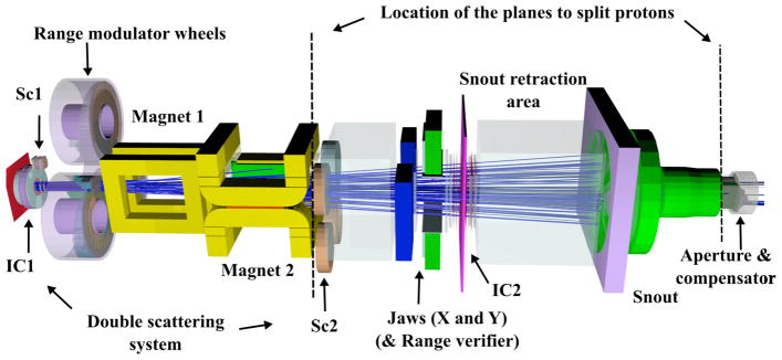
The FHBPTC treatment head as simulated with TOPAS with two split planes (dotted lines) located at upstream of the second scatterer (Sc2) and upstream the aperture. The proton beam (blue lines) follows the z-axis from left to the right.

Figure 2.

The UCSFETF proton beam line for eye treatment as simulated using TOPAS. Two split planes (dotted lines) located at upstream the Water column and upstream the 5th collimator (Coll) and aperture. The proton beam (blue lines) follows the z-axis from left to right.

In both settings, phase space (PHSP) files were generated at the distal end of the aperture for subsequent dose calculation in a water phantom located immediately downstream of the aperture. The reference data for both settings were generated by simulating 5 million histories of primary protons per CPU with a production cut of 0.05 mm (see section 2.3). A multiprocessor Linux cluster of 30 CPUs with 2.66 GHz Intel Xeon processors was used.

For the FHBPTC setups, the deposited dose in water was calculated from the PHSPs by using a water phantom of 18 × 18 × 38.9 cm³ divided into 90 × 90 × 389 voxels. A wall of Lexan of thickness 5.5 mm was located between the PHSP and the phantom surface. For the UCSFETF setup, the deposited dose was calculated in an 8 × 8 × 4 cm³ water phantom divided into 80 × 80 × 80 voxels. A wall of Plexiglas of thickness 1 mm was located between the phase space and the phantom surface. In both setups, the step size limit was set to 0.5 mm and no VRTs were applied for dose calculations.

The optimal parameters for several efficiency improvement techniques (EITs); that is, the combination of VRT and other approximations to improve the efficiency, including the number of split particles per source particle (the split number), the production cut value and the number of times the PHSPs were re-used (the multiple-use number) were studied. Note that for the variance-reduced simulations the number of primary protons is lower than for the reference simulations.

2.2 The patient geometry

For the FHBPTC, a patient CT data set (head and neck) was used to determine the performance of the EITs when using the PHSP for patient specific dose calculations. TOPAS provides a conversion from CT data (Hounsfield numbers) to materials and densities [10], [11]. A field with a modulation of 10.0 cm and a range of 12.5 cm was used. The corresponding aperture and compensator based on the treatment plan were included and the PHSPs were scored downstream of the compensator. The CT data consists of 512 × 512 × 76 voxels of 0.781 × 0.781 × 2.5 mm³ dimension.

2.3 The efficiency improvement techniques

Geometrical splitting with Russian roulette

Particle splitting and Russian roulette have been used in Monte Carlo simulations in x-ray and electron therapy [18], [19], and [20]. We have previously implemented the geometrical splitting technique (GST) in TOPAS [4], adapted to the specific needs of the passive-scattering proton therapy simulations. In this technique, N_s protons are generated (split) from the incident proton at planes perpendicular to the beam axis at specific positions in the treatment head. Further, prior to splitting, protons with low probability of contributing to the scoring region are subject to Russian roulette with a probability of discarding the particle equal to 1 – 1/N_s. The weight of the surviving protons is multiplied by a factor of 1/N_s. In regions with cylindrical symmetry, the position and momentum of each new proton is distributed to N_s different locations randomly rotated about the axis of symmetry (z-axis). The splitting utilized parallel geometries in Geant4.

With N_p source protons incident on the treatment head for the reference simulations without GST, the number of source protons for simulations with GST with two split planes was set to N_p/N_s2 to reach approximately the same number of protons at the phase space plane. Consequently, the simulation time for dose calculations was similar for simulations with and without GST.

For the FHBPTC setups, there were two split planes, one located upstream of the second scatterer, the other upstream of the aperture (Figure 1). The split numbers can be optimized for different geometries and are thus expected to be different for the FHBPTC setups and the UCSFETF setup. Based on our previous work [4], two split planes were used for the UCSFETF setup as well, but further studies were performed to determine the optimum location of the first plane. Four candidate locations were considered at upstream wide of the following components: The first ionization chamber (IC1), the propeller, the water column and the second ionization chamber (IC2) (Figure 2). Cylindrical symmetry was assumed at the aperture and PHSPs were generated downstream of the aperture for the FHBPTC and UCSFETF cases.

The energy fluence of protons at a PHSP was used to calculate the statistical uncertainty of the simulation and subsequently the computational efficiency (see section 2.4). For this purpose, the PHSPs were divided into concentric rings of equal area with a maximum radius of 5.7 cm (50 bins) and 1.25 cm (30 bins) for FHBPTC and UCSFETF setups respectively. To show the effect of Russian roulette in both setups, the radius of the user-defined region located at the phase space scoring plane was increased in multiplicative factors of the corresponding aperture radius. The energy fluence in each ring was calculated for several factors and compared against reference simulations. We rejected a setup with a difference of 1% of the maximum energy fluence.

Production cuts

The cut for the production of secondary particles refers to a threshold value of energy, such as EGSnrc [21], or secondary range, such as Geant4. A secondary particle is not tracked if the secondary to be created after a physical interaction has an energy or projected range below this threshold. It has been shown that the tracking of secondary particles other than protons at the treatment nozzle does not significantly alter the deposited dose in a phantom and can increase the computational efficiency by a factor of ~1.7 [22], [4]. In [4] particles other than protons are terminated once they were created, however, their production still needs considerable simulation time. One can tune the production cuts to avoid this step, however, excessively high production cuts can lead to systematic errors in the dose profiles or fluence profiles. In TOPAS production cuts are defined in units of length. The default value is set to 0.05 mm for electrons, positrons and photons. In this work, we optimize the production cut by increasing its value and by evaluating the computational efficiency for fluence profiles at the PHSP.

Multiple use of PHSPs

PHSPs are used multiple times for dose calculations to reduce the size of the PHSP file needed to achieve the desired statistical precision. This also reduces the time needed to calculate the PHSP. This is important in proton therapy as the treatment head geometry is patient dependent. The optimal number of times to use the same PHSP has been chosen by evaluating the statistical uncertainty of depth dose profiles versus the multiple-use number [18]. In order to maintain statistical accuracy, it is important to ensure that sufficient independent particle histories are included in the PHSP [23], otherwise systematic effects can be introduced. In photon therapy, the multiple-use number can be of the order of several hundreds [24], limited by the latent variance of the PHSP [19]. On the other hand, For proton therapy, the number of allowed multiple-uses can be much lower than for photon therapy because unlike photons, charged particles effectively lose energy continuously which can lead to larger systematic errors for the same numbers of multiple-use. For example, a maximum recycling of 4 has been recommended for electron beams [23]. To find the most suitable multiple-use number for each setup, the PHSP was generated from five million source protons and scored downstream of the aperture for four separate simulations with different random number seeds. For the FHBPTC setups the dose was scored into 6 × 6 × 0.1 cm³ volumes along the z-axis. For the UCSFETF setup, the dose was averaged over 1 × 1 × 0.05 cm³ volumes along the z-axis.

2.4 Computational efficiency and statistical uncertainty

With EITs there is a relationship between computation time (CPU time) and the statistical uncertainty, which needs to be optimized depending on the geometrical framework and the aim of the simulation. This relationship is specified by the computational efficiency ε [25]:

$$\epsilon =\frac{1}{s^{2}T},$$ (1)

where s is an estimate of the statistical uncertainty on the quantity of interest and T is the CPU time required to obtain this uncertainty. Previously, we developed an analytical expression to equation 1 by considering only one split plane [4]. For two split planes, the follow expression was inferred to describe the shape of the efficiency as a function to the number of splits:

$$\epsilon =\frac{{\epsilon }_0{N}_s^2}{\alpha +\beta N_s+\gamma N_s^2},$$ (2)

where ε₀ is the computational efficiency without any EIT, N_s is the number of splits and α, β and γ are the fraction of simulation time (with respect to the total simulation time in the treatment head) expended between the first split plane and the source, the second split plane and the first split plane, and the phase space plane and the second split plane, respectively (with α+β+γ = 1). The validity of a simulation with a split number of N_s will be subject to different parameters such as the number of source protons, the number of scored protons, and the simulation time. A very low number of source protons with a high N_s will lead to systematic errors because of the lack of particles with different characteristics (kinetic energy, spatial distribution, momenta, etc.), although the simulation time will be short.

To evaluate the overall uncertainty of the quantity of interest, the average statistical uncertainty s_Y as a measure of the overall statistical uncertainty s was obtained by [25]

$$s_{Y\%}^2=\frac{1}{N}\sum _{i=1}^N{\left(\frac{\delta X_i}{X_i}\right)}_{Y\%}^2,$$ (3)

where X_i is the quantity of interest (dose, deposited energy or fluence) in voxel i and δX_i is the corresponding statistical uncertainty. Only those voxels with a value larger than Y% of the maximum value are accounted for. Several values of Y have been proposed depending on the level of accuracy required [26]. For this work the most common value of 50% was used.

The accuracy of the variance-reduced simulations can be approximated by using the point-to-point relative percentage difference. In this work, this quantity was calculated to compare the planar fluence distribution and the dose profiles with and without a EIT. The set criterion of acceptance was that all values must be within 2% of the values from the reference simulation. An alternative comparison method is to perform the gamma index [27]. The gamma index test was calculated for complex dose distributions, such as the deposited dose in a patient. It has been stated that the quality assurance in intensity modulated proton therapy treatments should yield > 90% agreement for 3% and 3 mm criteria when doing a gamma analysis [28]. In this work, this criterion of acceptance was used as benchmark for dose calculation in the patient geometry. An additional comparison for the patient dose distributions was performed applying a method introduced by Kawrakow and Fippel [29]. The procedure calculates the difference x_ijk at the voxel ijk measured in units of the combined statistical uncertainty ΔX_ijk:

$$x_{\mathit{ijk}}=\frac{X_{\mathit{ijk}}^{\mathit{REF}}-X_{\mathit{ijk}}^{\mathit{EVAL}}}{\mathrm{\Delta }{X}_{\mathit{ijk}}}.$$ (4)

If the differences between X^REF and X^EVAL were purely statistical, then the probability distribution f(x) to find a voxel with a deviation given by x would be fit with a Gaussian function centered at zero. Otherwise, systematic errors are present. With sufficient moments of the distribution x, the amplitude and frequency of the voxels with systematic error can be found. Kawrakow and Fippel [29] provide a fitting function to interpret the x distribution in terms of its first four moments described as:

$$f(x)=\frac{1}{\sqrt{2\pi }}\left[{\alpha }_{1}exp\left(-\frac{{(x-{\delta }_1)}^2}{2}\right)+{\alpha }_{2}exp\left(-\frac{{(x-{\delta }_2)}^2}{2}\right)+(1-{\alpha }_1-{\alpha }_2)exp\left(-\frac{x^2}{2}\right)\right].$$ (5)

In simple terms, a fraction α₁ of the voxels have a systematic deviation δ₁ between the two dose distributions, while another fraction α₂ has a systematic deviation δ₂ between the two distributions. The actual maximum difference between the two distributions is obtained by multiplying the combined statistical uncertainty by the corresponding δ terms [30].

3 Results

3.1 Geometrical particle splitting

Results for particle splitting using the FHBPTC setups were reported previously [4]. The split number was fixed to 8 and cylindrically symmetry was assumed upstream of the aperture. We thus limit this section to the UCSFETF setup. The computational efficiency versus the number of splits is shown on the left side of Figure 3. For each curve, the location of the first plane was varied, i.e. set upstream of the first ionization chamber (IC1), the propeller, the water column, and the second ionization chamber (IC2). In all cases the second split plane was located upstream of the aperture. The larger gain in efficiency is obtained by placing the first split plane upstream of the water column or IC2. This is because the corresponding β parameter of Equation 2 (0.30 and 0.02 for the water column and the IC2 respectively) are shorter than for the others options (0.52 and 0.47 for the IC1 and the propeller respectively). On the right side of Figure 3 the depth-dose curves in water for two different locations of the first split plane (upstream of the water column and upstream of the IC2) were calculated for N_s equal to 16. Although the computational efficiency for the plane at the IC2 (157.1±3.8) is larger than the computational efficiency for the plane at the water column (111.8±2.5), the maximum difference (> 2%) near 2.6 cm is achieved with the former configuration. Between the split plane upstream the IC2 and the scoring region (PHSP) the only material is air. A lack of significant scattering in air will cause secondary protons created by splitting to likely reach the PHSP with the same characteristics. At this point, we therefore set the configuration for GST for the UCSFETF setup as: eliminate the particles different than protons along the track, a split plane upstream of the water column, a split plane upstream of the aperture, and a N_s of 16.

Figure 3.

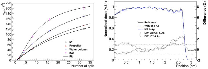
The computational efficiency values versus the number of splits (left) for the UCSFETF setup. The first plane was located either at the first ionization chamber (IC1), the propeller, the water column, or the second ionization chamber (IC2). In all cases the second split plane was located upstream of the aperture. The right panel shows the effects on dose profiles for N_s equal to 16 and two locations of the first split plane, i.e. at the water column and at the IC2. The differences in percent are shown on the right axis.

3.2. Effect of the radius of the region of interest in Russian roulette

The normalized energy fluence at radial position for several selected values of the diameter of the user-defined region for Russian roulette (RRR) is shown in Figure 4 and Figure 5 for the FHBPTC (two options) and UCSFETF setups, respectively. The results are presented relative to the reference simulation (without Russian roulette) and for different values for the fraction of the aperture radius. For the FHBTPC setups, we define the radius of the aperture as the distance from the center to a corner of the squared aperture. For FHBPTC-A1 and FHBPTC-A8, RRR equals to 2.0 and 1.25 times the radius of the aperture respectively, there are systematic errors introduced by the Russian roulette. The low energy protons, which contribute to the penumbra of the beam, will be scattered along the treatment head at higher angles in comparison with the source protons. When the diameter of the RRR is small, these low energy protons are discarded causing a lack of fluence near the boundary of the aperture region as depicted in Figure 4. The initial energy of the proton beam for the FHBPTC setups (~173 MeV and ~214 MeV) is larger than for the UCSFETF setup (~67 MeV). Thus, the ratio between the radius of RRR and the radius of the aperture for the FHBPTC setups have to be defined smaller than for the UCSFETF setup. If a constraint of 1% in the difference for the planar fluence is required, then for the FHBPTC-A1 and FHBPTC- A8 setups, diameters of RRR of 2.5 and 1.5 times the radius of the aperture are adequate with an efficiency gain of 1.29±0.03 and 1.45±0.06, which represents a time reduction of about 21.2%±0.2% and 40%±0.1%, respectively. Since the initial beam energy (and thus beam scattering) at the FHBPTC is treatment field dependent, this RRR diameter is field dependent. On the other hand, for the UCSFETF setup an efficiency of 1.25±0.02 (20%±0.3% of time saving) is achieved for the adequate diameter of RRR equal to 4 times the radius of the corresponding aperture. It is important to note that the gain in efficiency is with respect to the geometrical particle split with the option of eliminating all particles other than protons.

Figure 4.

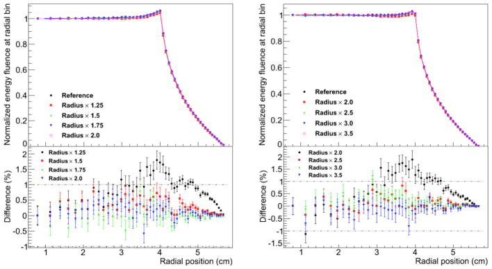
Normalized energy fluence at radial position for FHBPTC-A1 (left) and FHBPTC-A8 (right). Several values for the diameter of the region of the Russian roulette are compared. Differences in percent are shown at the bottom.

Figure 5.

Normalized energy fluence at radial position for UCSFETF. Several values for the diameter of the region of the Russian roulette are compared. Differences in percent are shown at the bottom.

3.3. Production cuts and multiple-use of PHSP

Figure 6 illustrates the effect on the computational efficiency by varying the production cut for the FHBPTC setups. As depicted there exists a maximum in the computational efficiency at 500 mm (albeit with significant error bars). On the other hand, if the simulation time is considered, a saturation point at 50 mm is achieved. This value was thus chosen for the FHBPTC setups. The effect on the precision of the simulation is the introduction of systematic errors if the production cut is too high. For the FHBPTC setups there is no effect on the precision when increasing the production cut, as will be shown in section 3.5. On the other hand, for the UCSFETF setup, an increase in the production cut leads to increasing differences in the energy fluence at radial position profiles, as depicted in Figure 7. Thus, the contribution of the secondary electrons, positrons and gammas are more important at this beam energy (~67 MeV). For a production cut value of 2.0 mm the differences with respect to the reference simulation would be acceptable (in energy fluence profiles at PHSP we consider that the condition is satisfied for values lower than 1%), however the reduction in computation time is only about 6%. A significant reduction in the CPU time is achieved for a 2.8 mm of production cut, however the differences are higher than 1.5%. Therefore, the production cut for UCSFETF setup was fixed to the default value: 0.05 mm. The scattering system plays an important role in the difference between production cuts of the two facilities. For FHBPTC setups a double scattering system is present, whereas for the UCSFETF setup a scattering system was not present.

Figure 6.

Normalized computational efficiency (solid lines and left axis) and CPU time in minutes (dotted lines and right axis) for the FHBPTC setups. The statistical uncertainty of energy fluence was used to calculate the efficiency.

Figure 7.

Average relative difference of the energy fluence at radial position (squares) and relative simulation time to the reference simulation time (circles) for the UCSFETF

Figure 8 shows the statistical uncertainty versus the multiple-use number for the PHSP. For both the FHBPTC (two options) and UCSFETF setups, the uncertainty is reduced as the multiple-use number increases by following a power la fit (power of −1.35, −0.9 and −1.08 for FHBPTC-A1, FHBPTC-A8 and UCSFETF respectively). For the FHBPTC setups, a reduction of 27% (FHBPTC-A1) and 42% (FHBPTC-A8) in the statistical uncertainty is achieved for a multiple-use of 4 (with a simulation time increase by a factor of 4). For the UCSFETF setup, a reduction of 18% in statistical uncertainty is achieved for a multiple-use of 2. After a multiple use of 2, the reduction is reaching a plateau. Thus, the number of multiple-use of PHSPs for dose calculations was set to 4 for FHBPTC and 2 for UCSFETF setups respectively.

Figure 8.

Fractional uncertainty in energy fluence for the inner ring versus number of multiple-use of the phase space.

3.4. Calculation of 3D-Dose distributions

The accuracy of the PHSP data obtained with the configurations considered in the previous sections was evaluated by calculating dose distributions in water and in a patient. The EIT configurations for the FHBPTC and UCSFETF setups are shown in Table 1. These parameters are used for the generation of the PHSPs only.

Table 1.

Optimal parameters for efficiency improvement for the FHBPTC and UCSFETF setups.

	Split planes at upstream of	Ns	Russian roulette Aperture radius factor	Production cut (mm)	Multiple-use
FHBPTC-A1	Sc2, Aperture	8	2.5	50.0	4
FHBPTC-A8	Sc2, Aperture	8	1.5	50.0	4
Patient	Sc2, Aperture	8	1.5	50.0	4
UCSFETF	Water column, Aperture	16	4.0	0.05	2

In Figures 9, 10 and 11 the dose profiles from the 3D distributions for the FHBPTC setups and the UCSFETF setup are shown respectively. For the FHBPTC setups, the differences with respect to the reference simulations are below 2% for the lateral profiles and below 1.5% for depth profiles. For the UCSFETF setup, the differences are below 2% for the lateral profiles and below 1% for depth profiles. In both setups, the profiles were normalized to the maximum value in the SOBP region.

Figure 9.

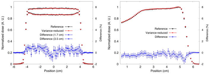
Dose profiles for FHBPTC-A1. Lateral dose profile (left) at 1.7 cm and 3.5 cm from the entrance of the water phantom. The depth-dose profiles are shown the right. Percentage differences are also shown.

Figure 10.

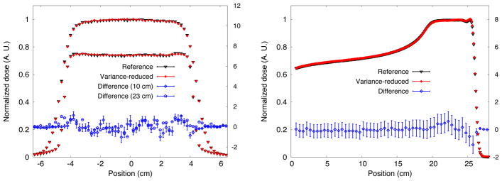
Dose profiles for FHBPTC-A8. Lateral dose profile (left) at 10 cm and 23 cm from the entrance of the water phantom. The depth-dose profiles are shown the right. Percentage differences are also shown.

Figure 11.

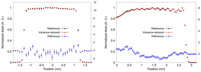
Lateral dose profile (left) at maximum depth-dose (right) for UCSFETF. Percentage differences on the right axis are also shown.

The iso-dose line representation of the dose distribution at the transverse plane of the head and neck example is shown in Figure 12. For the full dose distributions and only for those voxels with dose larger than 20% of the maximum, 98.4% of voxels had a gamma value lower than unity (2% and 2 mm criteria), 99.9% if the criteria is 3% and 3mm.

Figure 12.

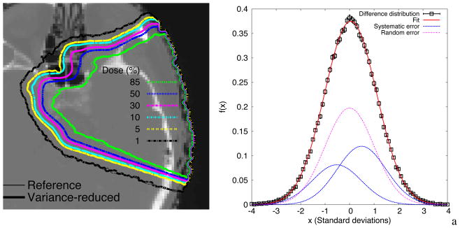
Transverse view of the dose distribution in a patient head. The left shows the fit to equation 5. fraction α₁=0.29 of the voxels show a systematic difference δ₁=0.49 standard deviations. A fraction of α₂=0.2 of voxels show a systematic difference δ₂=−0.52 standard deviations. The rest of the voxels show no systematic differences.

The procedure described in Section 2.4 was used to compare the patient dose distributions. Figure 13 shows a fit of Equation 5 to the difference distribution, i.e. Equation 4. Only voxels with dose greater than 20% were included. A fraction α₁ = 0.29±0.06 of the voxels from the efficiency-improved simulation systematically predicted a lower dose by δ₁ = 0.49±0.06 standard deviations compared to the reference simulations. Another fraction α₂ = 0.2±0.07 shows efficiency-improved simulations systematically predicting a dose lower by δ₂ = −0.52±0.03 standard deviations compared to the reference simulations. The remaining proportion of voxels showed no systematic differences between the distributions. If the combined statistical uncertainty was about 1.7%, then a fraction α₁ of the voxels showed a systematic difference of 0.83% of the maximum dose, while a fraction α₂ of the voxels showed a systematic difference of 0.88% of the maximum dose.

As a final result, in Table 2 the average CPU time in minutes and the normalized computational efficiency are shown.

Table 2.

Average CPU time and normalized computational efficiency. The planar fluence was considered to calculate the average statistical uncertainty for voxels with 50% of the maximum value.

Option	Average CPU Time (min)		Efficiency normalized to the reference simulation
	Reference	With EIT
FHBPTC-A1	512.8 (2.2)	10.21 (0.03)	51.25 (0.04)
FHBPTC-A8	543.2 (5.7)	28.3 (0.1)	19.9 (0.1)
Patient	569.8 (1.9)	6.82 (0.01)	78.6 (7.5)
UCSFETF	559.8 (5.5)	10.2 (0.1)	57.3 (0.5)

4 Discussion

In this work, the optimal parameter settings for EITs when generating phase spaces in proton therapy simulations were studied for two very different treatment heads. The computational efficiency and direct comparison of dose profiles were made for water phantom and patient cases. From our previous work [4], geometrical based particle splitting for the FHBPTC setup resulted in normalized computational efficiency improvements of a factor of 10 to 20.3. In this work we have expanded on this study to include a study of the Russian roulette technique and production cuts and the application of these techniques to another treatment head. First, the studies performed in this work, allow quantification of the contribution to the gain in efficiency for Russian roulette: A factor of 1.45±0.06 and 1.25±0.02 for the FHBPTC and UCSFETF setups, respectively. Note that, strictly speaking, Russian roulette is not a VRT [8] because of the introduction of bias in the fluence profiles. However, with judicious choice of the size of the Russion roulette region, it is possible to reduce the computation time without compromising accuracy. Second, for the FHBPTC facility, with proton ranges from 4.79 cm up to 27.88 cm, high production cuts (higher than 50 mm) can be applied within the treatment head, allowing a reduction of the simulation time up to 40% (efficiency gain of 1.6±0.2). For patient dose calculations the production cut should be set to 0.05 mm. On the other hand, for simulations of treatment heads using lower proton energies (e.g. to treat ocular melanoma as in the case of the UCSFETF setup), an increase of the production cut which leads to significant simulation time reduction (>2.0 mm), causes a significant bias in the energy fluence profiles (>1.5%). With lesser restrictions in the maximum difference allowable, further efficiency gains from a higher production cut could be achieved. For example, with a restriction of 2% in energy fluence, a reduction up to 20% in CPU time could be achieved. In any case, the gain in efficiency due to geometrical particle split and Russian roulette configuration is still significant (57.3 for the proposed configuration).

For the particle splitting settings described in [4], a minimum gain in efficiency (a factor of ~10) was achieved. In this work a minimum gain in efficiency was a factor of 20 for the setups of the FHBPTC, i.e. the efficiency was doubled. For a head patient dose calculation, the gain in efficiency was about a factor of 80. The maximum systematic difference of 0.88% was found for voxels with 20% of the maximum dose or more. The use of equation 5 [29] allowed to quantify the degree of bias introduced, primarily by the production cut. The gamma index test (98.4% for 2% and 2 mm criteria in this study) does not allow to separate such systematical differences from statistical differences.

The simulation time depends on the voxel size (the voxel size in our patient example was 0.78×0.78×2.5 mm³). Further reduction in computation time can be achieved to achieve the same statistical precision if larger voxels are used. Also, post-processing of dose distributions using denoising techniques can allow further reduction of the number of source protons needed to reach the desired precision as in the case of conventional radiotherapy simulations [31].

5 Conclusions

Optimal parameters for several variance reduction techniques and approximations have been obtained for different geometries in passive scattering mode, which cover the range of application for proton therapy, one for eye treatment (UCSFETF) and one for high energy beam delivery (FHBPTC). For PHSP simulations in the case of the FHBPTC setup the inclusion of two split planes (split number of 8) with a radius of 1.5–2.5 times the radius of the aperture, and a production cut of 50 mm for secondary particles (electrons mainly) resulted in an enhancement of efficiency of factors between 20 and 78 without a clinically meaningful loss of accuracy. For the UCSFETF setup, two split planes (split number of 16) with a radius of 4 times the radius of the corresponding aperture, and eliminating the secondary particles other than protons, efficiency gains up 57.3 were achieved. By using these techniques with the optimal parameters obtained in this work, dose distributions in homogeneous and heterogeneous volumes agreed within acceptable clinical tolerance when comparing with reference simulations produced with the TOPAS code.

References

- 1.Cygler JE, Lochrin C, Daskalov GM, Howard M, Zohr R, Esche B, Eapen L, Grimard L, Caudrelier JM. Clincal use of a commercial Monte Carlo treatment planning system for electron beams. Phys Med Biol. 2005;50(5):1029–1034. doi: 10.1088/0031-9155/50/5/025. [DOI] [PubMed] [Google Scholar]
- 2.Ma CM, Mok E, Kapur A, Pawlicki T, Findley D, Brian S, Foster K, Boyer AL. Clinical implementation of a Monte Carlo treatment planning system. Med Phys. 2009;26(10):2133–2143. doi: 10.1118/1.598729. [DOI] [PubMed] [Google Scholar]
- 3.Fan J, Luo W, Fourkal E, Lin T, Li J, Veltchev I, Ma CM. Shielding design for a laser- accelerated proton therapy system. Phys Med Biol. 2007;52(13):3913–3930. doi: 10.1088/0031-9155/52/13/017. [DOI] [PubMed] [Google Scholar]
- 4.Ramos-Méndez J, Perl J, Faddegon B, Schuemann J, Paganetti H. Geometrical splitting technique to improve the computational efficiency in Monte Carlo calculations for proton therapy. Med Phys. 2013;40(4):041718. doi: 10.1118/1.4795343. [DOI] [PMC free article] [PubMed] [Google Scholar]
- 5.Sawakuchi GO, Mirkovic D, Perles LA, Sahoo N, Zhu XR, Ciangaru G, Suzuki K, Gillin MT, Mohan R, Titt U. An MCNPX Monte Carlo model of a discrete spot scanning proton beam therapy nozzle. Med Phys. 2010;37(9):4960–4970. doi: 10.1118/1.3476458. [DOI] [PMC free article] [PubMed] [Google Scholar]
- 6.Sawakuchi GO, Titt U, Mirkovic D, Ciangaru G, Zhu XR, Sahoo N, Gillin MT, Mohan R. Monte Carlo investigation of the low-dose envelope from scanned proton pencil beams. Phys Med Biol. 2010;55(3):711–721. doi: 10.1088/0031-9155/55/3/011. [DOI] [PubMed] [Google Scholar]
- 7.Ali ESM, Rogers DWO. Efficiency improvements of X-Ray simulations in EGSnrc user-codes using bremsstrahlung cross-section enhancement (BCSE) Med Phys. 2007;34:2143–2154. doi: 10.1118/1.2736778. [DOI] [PubMed] [Google Scholar]
- 8.Bielajew A, Rogers DWO. Variance-Reduction Techniques in Monte Carlo Transport of Electrons and Photons. Plenum; New York: 1998. pp. 407–419. [Google Scholar]
- 9.Wulff I, Zink K, Kawrakow I. Efficiency improvements for ion chamber calculations in high energy photon beams. Med Phys. 2008;35(3):1328–1336. doi: 10.1118/1.2874554. [DOI] [PubMed] [Google Scholar]
- 10.Perl J, Shin J, Schuemann J, Faddegon B, Paganetti H. TOPAS an innovative proton Monte Carlo platform for treatment head and patient simulations in research and clinical applications. Med Phys. 2012;39(11):6818–6837. doi: 10.1118/1.4758060. [DOI] [PMC free article] [PubMed] [Google Scholar]
- 11.Schuemann J, Paganetti H, Shin J, Faddegon B, Paganetti H. Efficient voxel navigation for proton therapy dose calculation in TOPAS and Geant4. Phys Med Biol. 2012;57:3281–3293. doi: 10.1088/0031-9155/57/11/3281. [DOI] [PMC free article] [PubMed] [Google Scholar]
- 12.Shin J, Perl J, Schuemann J, Paganetti H, Faddegon B. A modular method to handle multiple time-dependent quantities in Monte Carlo simulations. Phys Med Biol. 2012;57:3295–3308. doi: 10.1088/0031-9155/57/11/3295. [DOI] [PMC free article] [PubMed] [Google Scholar]
- 13.Agostinelli S, et al. Geant4: a simulation toolkit. Nucl Instrum Methods Phys Res A. 2003;506:250– 303. [Google Scholar]
- 14.Paganetti H, Jiang H, Parodi K, Slopsema R, Engelsman M. Clinical implementation of full Monte Carlo dose calculation in proton beam therapy. Phys Med Biol. 2008;53:4825–4853. doi: 10.1088/0031-9155/53/17/023. [DOI] [PubMed] [Google Scholar]
- 15.Paganetti H, Jiang HH, Lee SY, Kooy HM. Accurate Monte Carlo simulations for nozzle design, commissioning and quality assurance for a proton radiation therapy facility. Med Phys. 2004;31(7):2107–2118. doi: 10.1118/1.1762792. [DOI] [PubMed] [Google Scholar]
- 16.Daftary IK, Renner TR, Verhey LJ, Singh RP, Nyman M, Petti PL, Castro JR. New UCSF proton ocular beam facility at the Crocker Nuclear Laboratory Cyclotron (UC Davis) Nucl Instrum Methods Phys Res A. 1996;380:597–612. [Google Scholar]
- 17.Jarlskog CZ, Paganetti H. Physics settings for using the Geant4 toolkit in proton therapy. IEEE Trans Nucl Sci. 2008;55(3):1018–1025. [Google Scholar]
- 18.Kawrakow I, Rogers DWO, Walters BRB. Large efficiency improvements in BEAMnrc using directional splitting. Med Phys. 2004;31(10):2883–2898. doi: 10.1118/1.1788912. [DOI] [PubMed] [Google Scholar]
- 19.Sempau J, Sánchez-Reyes A, Salvat F, Oulad ben Tabar H, Jiang SB, Fernández-Varea JM. Monte Carlo simulation of electron beams from an accelerator head using PENELOPE. Phys Med Biol. 2001;46:1163–1186. doi: 10.1088/0031-9155/46/4/318. [DOI] [PubMed] [Google Scholar]
- 20.Ma CM, Li JS, Pawlicki T, Jiang SB, Deng J, Lee MC, Koumrian T, Luxton M, Brain S. A Monte Carlo dose calculation tool for radiotherapy treatment planning. Phys Med Biol. 2002;47(10):1671–1690. doi: 10.1088/0031-9155/47/10/305. [DOI] [PubMed] [Google Scholar]
- 21.Kawrakow I. Accurate condensed history Monte Carlo simulation of electron transport. I. EGSnrc, the new EGS4 version. Med Phys. 2000;27(3):485–498. doi: 10.1118/1.598917. [DOI] [PubMed] [Google Scholar]
- 22.Paganetti H. Nuclear interactions in proton therapy: dose and relative biological effect distributions originating from primary and secondary particles. Phys Med Biol. 2002;47:747–764. doi: 10.1088/0031-9155/47/5/305. [DOI] [PubMed] [Google Scholar]
- 23.Kawrakov I, Walters BRB, Rogers DWO. The history by history statistical estimators in the BEAM code system. Med Phys. 2002;29:2745–2752. doi: 10.1118/1.1517611. [DOI] [PubMed] [Google Scholar]
- 24.Bush K, Zavgorodni S, Beckham W. Azimuthal particle redistribution for the reduction of latent phase-space variance in Monte Carlo simulation. Phys Med Biol. 2007;52:4345–4360. doi: 10.1088/0031-9155/52/14/021. [DOI] [PubMed] [Google Scholar]
- 25.Rogers DWO, Mohan R. Questions for comparison of clinical Monte Carlo codes. In: Bortfeld T, Schlegel W, editors. Proceedings of the 13th ICCR. Springer-Verlag; 2000. pp. 120–122. [Google Scholar]
- 26.Fragoso M, Kawrakow I, Faddegon B, Solberg T, Chetty I. Fast, accurate photon beam accelerator modeling using BEAMnrc: a systematic investigation of efficiency enhancing methods and cross-section data. Med Phys. 2009;36(12):5451–5466. doi: 10.1118/1.3253300. [DOI] [PMC free article] [PubMed] [Google Scholar]
- 27.Low D, Harms W, Mutic S, Purdy J. A technique for the qualitative evaluation of dose distributions. Med Phys. 1998;25(5):656–661. doi: 10.1118/1.598248. [DOI] [PubMed] [Google Scholar]
- 28.Titt U, Bednarz B, Paganetti H. Comparison of MCNPX and Geant4 proton energy deposition predictions for clinical use. Phys Med Biol. 2012;57:6381–6393. doi: 10.1088/0031-9155/57/20/6381. [DOI] [PMC free article] [PubMed] [Google Scholar]
- 29.Kawrakow I, Fippel M. Investigation of variance reduction techniques for Monte Carlo photon dose calculation using XVMC. Phys Med Biol. 2000;45:2163–3184. doi: 10.1088/0031-9155/45/8/308. [DOI] [PubMed] [Google Scholar]
- 30.Gardner J, Siebers J, Kawrakow I. Dose calculation validation of VMC++ for photon beams. Med Phys. 2007;34(5):1809–1818. doi: 10.1118/1.2714473. [DOI] [PubMed] [Google Scholar]
- 31.El Naqa I, Kawrakow I, Fippel M, Siebers JV, Lindsay PE, Wickenhauser MV, Vicic M, Zakarian K, Kauffmann N, Deasy JO. A comparison of Monte Carlo dose calculation denoising techniques. Phys Med Biol. 2005;50:909–922. doi: 10.1088/0031-9155/50/5/014. [DOI] [PubMed] [Google Scholar]