In Vivo Axial Loading of the Mouse Tibia

Summary

Non-invasive methods to apply controlled, cyclic loads to the living skeleton are used as an anabolic agent to stimulate new bone formation in adults and enhance bone mass accrual in growing animals. These methods are also invaluable for understanding bone signaling pathways. Our focus here is on a particular loading model: in vivo axial compression of the mouse tibia. An advantage of loading the tibia is that changes are present in both the cancellous envelope of the proximal tibia and the cortical bone of the tibial diaphysis. To load the tibia of the mouse axially in vivo, a cyclic compressive load is applied up to five times a week to a single tibia per mouse for a duration lasting from 1 day to 6 weeks. With the contralateral limb as an internal control, the anabolic response of the skeleton to mechanical stimuli can be studied in a pairwise experimental design. Here, we describe the key parameters that must be considered before beginning an in vivo mouse tibial loading experiment, including methods for in vivo strain gauging of the tibial midshaft, and then we describe general methods for loading the mouse tibia for an experiment lasting multiple days.

1. Introduction

In the field of bone metabolism, considerable interest exists in elucidating new anabolic pathways that can be targeted therapeutically to improve bone mass and strength. The dysregulation of certain bone-active signaling pathways, manifest in numerous human diseases of bone metabolism as altered bone mass, size and strength, have shed light on the mechanisms of normal skeletal homeostasis. More importantly, these observations provide insight into viable molecular targets that can be manipulated in otherwise healthy patients to achieve a therapeutic outcome. Recent efforts in skeletal biology have been focused on uncovering new anabolic, rather than anti-catabolic, pathways that can be manipulated to improve bone mass in skeletally fragile individuals. In addition, certain skeletal diseases have yielded targets for anabolic action in bone (e.g. hyperostosis corticalis, sclerosteosis). However, a much more ubiquitous mechanism of bone formation and accrual, that is not based on disease yet is incredibly anabolic, is available for therapeutic discovery. That mechanism is mechanotransduction, the process by which bone responds and adapts to its mechanical environment by adjusting tissue mass, architecture and material properties.

Repeated increased loading, such as occurs with exercise, has the propensity to induce new bone formation. Conversely, when loads are reduced during conditions such as bed rest, neuromuscular paralysis, and spaceflight, bone mass is lost in the weight-bearing bones. Despite its anabolic potential, our understanding of the cellular and molecular mechanisms that govern this adaptive process is far from complete. To systematically study this process, and eventually identify and clearly define the anabolic mechanisms involved, reliable, meaningful, well-characterized, and reproducible physiologic models of mechanical loading are crucial, preferably in intact animals. Towards this end, a number of animal loading models have been developed, including rodent exercise studies, rodent whole body vibration, and in vivo loading models such as tibial four-point bending, rodent ulnar axial loading, and mouse tibial axial loading (1–6). An advantage of in vivo mechanical loading models is that controlled, repeated mechanical forces are applied to the skeletal site of interest. In contrast, exercise studies are associated with a mechanical environment that is much more difficult to quantify and is less well-controlled.

One in vivo loading model that has been met with broad appeal is the mouse tibial axial loading model. This model applies cyclic, physiologically relevant loads to one tibia while using the contralateral tibia as an internal control (3, 7). This model has several advantages, including the use of the mouse, and the presence of substantial volumes of cortical and cancellous bone. The mouse is a valuable animal model because of the opportunity to study genetic manipulations, including congenic, transgenic, knockout, and knock-in mice. These genetic models can provide critical insights into the underlying mechanisms involved in mechanotransduction. The mouse tibia can provide information about the skeletal response to applied loads across several bone envelopes: cancellous, periosteal, and endocortical.

This chapter describes general methods for cyclic loading of the mouse tibia. The loading can be performed using a load-controlled mechanical testing system or a custom loading device with Labview software. The basic protocol in our laboratories involves loading groups of mice under isoflurane anesthesia for multiple days, and the procedures described are generally applicable and can be modified to suit an investigator’s particular goals. Before beginning a loading experiment, a number of items must be considered. Loading protocols reported in the literature use a variety of different parameters including number of loading sessions per week, number of loading cycles per day, and characteristics of the load waveform including the loading frequency, loading rate, and inclusion of rest periods (8, 9). Maximum or peak compressive load must also be determined prior to loading by using in vivo strain gauging techniques to measure bone stiffness at the tibial midshaft. Furthermore, before loading experiments are underway, a sham loading experiment must be performed to confirm the lack of systemic effects in any particular laboratory set-up. These considerations are first described, followed by a general outline of the strain gauging procedures and in vivo axial tibial loading methods.

Although not the focus of this chapter, before beginning an experiment, relevant outcome measures must be chosen. This choice will affect experimental design, number of animals, and experiment duration. Common outcomes measures include gene expression via qPCR, bone geometry and morphology via micro-computed tomography, dynamic histomorphometry via injection of bone-seeking fluorescent labels prior to sacrifice, protein and/or RNA localization via immunohistochemistry or in situ hybridization, mechanical testing, serum measurements via ELISA or RIA, body and organ masses, and many others.

2. Materials

2.1 Animal Model Selection

1. Select mouse strain. The choice of background strain for mouse axial tibial loading will depend on a number of factors. The amount of cancellous bone in the tibial metaphysis varies with mouse strain, as do cortical bone mass, bone mineral density, bone shape, and bone strength (10–14). Tibia length and mouse size are also items to consider. Furthermore, some mouse strains are more mechanoresponsive than others (15, 16).

2. Select wild type or genetically modified mice. Depending on the research question, genetically modified mice may help identify whether the response to loading depends on the absence, presence, overexpression or modification of a particular gene or set of genes.

3. Select appropriate sex. The research question being asked will guide the decision regarding the use of male or female mice (or both). For example, models of post-menopausal osteoporosis are usually performed in female mice, particularly if ovariectomy will be used. Models of osteoarthritis usually use male mice because of the chondroprotective effect of estrogen (17). Many individual genes or larger quantitative trait loci (QTL) are associated with sex-specific effects, so when dealing with a novel gene or pathway with no a priori knowledge of sex interaction, males and females should both be studied.

4. Select mouse age. Again, this choice depends on the research question. Growing animals are still accruing bone mass, until around 16–24 weeks of age, when peak bone mass is reached although the specific age varies with bone site and mouse strain (11, 14). Aged mice are usually in a state of bone loss (18). Mice that have just reached skeletal maturity (e.g., 16 wks of age) are often used for tibia loading because the skeleton is still young enough to elicit a robust anabolic response to mechanical stimulation, and at the same time, the appositional growth on the periosteal surfaces has dropped to very low levels. This latter attribute allows for a less complicated interpretation of the load-induced bone formation effects observed in the loaded limb. At this age at this age the anabolic response is almost exclusively a result of loading, rather than a combined function of growth and enhanced mechanical input (as occurs in loaded growing bone).

2.2 Select appropriate controls

1. Sham controls. A separate experiment must be performed to ensure that tibial loading does not cause systemic effects, which have been both confirmed and refuted in the literature (19, 20). Confirm that paired contralateral control limbs from loaded mice are not different from control limbs obtained from separate nonloaded animals. This experiment should contain two groups of mice for an experimental duration corresponding to that of the planned in vivo tibial loading experiments. The first group of mice should have one tibia loaded while the contralateral limb is used as an internal control. The second group should be put under anesthesia and have one tibia placed in the loading device for the duration of loading just as the first group, but the tibia should not actually be loaded during the experiment (sham loading). If the results from the two sets of control limbs are similar, then paired contralateral limbs are appropriate controls.

2. Paired controls. If no systemic effects are presents, the contralateral, unloaded limb is often used as the control tibia, to which all measurable outcomes will be compared in determining bone’s anabolic response to mechanical loading.

2.3 Strain Gauging Materials (When not specified, materials can be ordered from Fisher Scientific or similar supplier)

1. 60/40 tin/lead solder, 0.022 inch diameter (Multicore Solders, Westbury, NY)

2. Three-conductor cable (Vishay Micro-Measurements, Wendell, NC, Cat# 336-FTE)

3. Soldering iron (GC Electronics, Rockford, IL, Model# 12-070)

4. Dissecting microscope with light source

5. Dissecting curved jewelers microforceps (Fisher Scientific, Cat# 08-953F)

6. Standard capacity wire stripping system (American Beauty, Clawson, MI, Model# 10503)

7. Tip tinner (MG Chemicals, Burlington, Ontario, Cat# 4910-28G)

8. Rosin Soldering Flux (Radio Shack)

9. Single element strain gauges (Vishay Micro-Measurements, Cat# EA-06-015LA-120)

10. Scalpel holder and #15 scalpel blades

11. Isopropyl alcohol

12. Clear tape

13. Index cards for gauge preparation

14. 1st coat: M Bond Adhesive Resin Type AE (Vishay Micro-Measurements)

15. Catalyst for 1st coat: M Bond Type 10 Curing Agent (Vishay Micro-Measurements)

16. 2nd coat: M Coat D (Vishay Micro-Measurements) (store in refrigerator)

17. 3rd coat: M Coat A (Vishay Micro-Measurements) (store in refrigerator)

18. Weigh boats in which to mix the first coat with the catalyst

19. Cotton swabs to apply isopropyl alcohol

20. Wooden applicator sticks to apply coat coverings

21. Eye dropper or transfer pipettes

22. Xylene, to thin 3rd coat if needed

23. Toluene, to thin 2nd coat if needed

24. Plugs for wires to connect gauge to computer or data acquisition device (Digi-Key, Thief River Falls, MN, Part# A26528-40-ND)

25. 1-min, 3-min, or 5-min curing epoxy

26. Digital multimeter

27. Strain conditioning hardware including bridge excitation, Wheatstone bridge circuit, and signal amplification and filtering. Integrated systems are produced by Vishay Micro-measurements and National Instruments LabView board (Part #’s 781156-01, 779521-01, 194738-01, 779012-01).

2.4 Surgical Supplies

1. Surgical tools including scissors, small scalpels and blades, jeweler’s forceps, periosteal elevator and small-tooth forceps

2. Small gauze

3. Small animal razor

4. Calipers

5. Cotton swabs

6. Methyl ethyl ketone

7. Cyanoacrylate tissue adhesive

2.5 Loading Materials

1. Loading device with actuator, calibrated load cell (or similar)

2. Computer with connections for loading hardware and electronics

3. If using custom loading device, signal conditioning hardware for data acquisition from load cell with Labview software for tibial loading (or similar) (see ^{Note 1})

4. Loading configuration files to input loading parameters

5. Wooden cylindrical rod (~17mm length) from long cotton swab handle (Fisher Scientific, #23-400-118) for loading program test (see ^{Note 2})

2.6 Mouse Care Materials

1. Rodent cages with food, enrichment (such as a shelter, PVC pipe, running wheel, or hard wood block), nesting material, and water.

2. Rodent anesthesia induction chamber

3. Mouse anesthesia nose cone

4. Isoflurane anesthesia machine with tubing attached to anesthesia chamber and mouse nose cone simultaneously

5. Oxygen tank connected to isoflurane machine

6. Isoflurane

7. Carbon cartridge halogen filters connected to tubing to scavenge isoflurane

8. Sterile petroleum jelly eye ointment (Fisher Scientific, Cat# NC0138063)

9. Extra mouse cage for anesthesia recovery

10. Balance with 0.01g accuracy and maximum capacity of at least 200g

3. Methods

All animal procedures should be reviewed and approved by your Institutional Animal Care and Use Committee.

Prior to Loading Experiment

3.1 Loading Parameter Selection

1. Select peak or maximum compressive load. Peak or maximum load is the load level that will be reached repeatedly during the cyclic loading. This load can vary depending on age, sex, strain, and genotype. To determine this load level, in vivo strain gaging at the tibial midshaft should be performed. (See 3.2 “Determining in vivo stiffness using strain gauges” below.) By determining tibial bone stiffness at the midshaft, the load to produce a desired strain at the tibial midshaft can be chosen.

2. Select pre-load value. The magnitude of the compressive pre-load should be a small percentage of the maximum or peak load. For example, −0.5N is an appropriate pre-load for a −9.0N compressive peak load (see ^{Note 3}).

3. Select frequency, loading rate, dwell time, and number of cycles for the loading waveform. Triangle waves are generally used because the load is applied at a constant strain rate. For a sinusoidal wave, the loading rate varies throughout the cycle. One commonly used in vivo compressive loading protocol for the mouse consists of 1200 cycles per day at 4 Hz, with a load-unload ramp of 0.15 seconds and 0.1s dwell time (Figure 1) (8). Another common protocol applies 60 cycles per day at 2Hz, with a load-unload ramp of 0.15 seconds and 10s second dwell time (9). (see ^{Note 4})

4. Select pause insertion duration. Bone formation is stimulated by inserting pauses in between load cycles, rather than continuous cyclic loading (21). In axial tibial loading of mice, rest insertions have been short (0.1s) or long (10.0s) (8, 9). As described in Step (3) pauses also can be used to achieve the desired loading rate and frequency.

5. Select loading duration. A range of loading durations have been used. Loading 3 or 5 times per week is most common (8, 9). The duration of loading experiments can last from 1 day to 6 weeks and will depend on the research question and outcome measurements. Shorter time frames are often used when the primary outcome measures are skeletal gene expression changes after mechanical loading. Longer time frames are often used to detect changes in bone morphology, geometry, and cellular activity.

Figure 1.

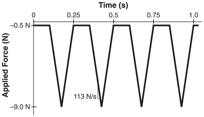
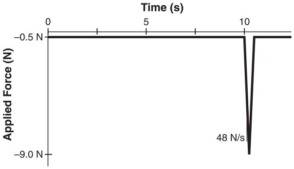
Common in vivo axial tibial loading triangular waveforms for mice with 9.0N peak compressive load. (A) This waveform is usually run 5 times per week, 1200 cycles per day at a rate of 4Hz, with a 0.1s dwell period, and 113 N/s loading rate (8). (B) This waveform is run 3 times per week, 60 cycles per day at a rate of 0.1Hz, with a 10.0s dwell period and a 48 N/s loading rate (9).

3.2 Determining in vivo stiffness using strain gauges

Strain gauges are electrical conductors that change resistance when deformed. By rigidly attaching a gauge to the surface of the tibia, the deformation caused by loading can be measured. Stiffness is then calculated as the applied load per deformation. In practice, the goal is to determine the load required to achieve a desired strain level on the bone surface. For a stiff bone, this load is higher than for a more compliant bone.

3.2.1 Strain gauge preparation (Figure 2)

Figure 2.

Trimmed strain gauge assembly. (A) Top view of strain gauge preparation. (B) Side-view schematic of strain gauge preparation. The 1^st coat is applied only to the soldering joint and should not touch the gauge grid. The 2^nd and 3^rd coats are applied to the entire gauge top surface. Stripped wire should not be exposed and can be covered by the coats.

1. Trim the gauge of unnecessary material. Place gauge on an index card and view using a dissecting microscope. Using a scalpel, remove excess material by cutting just within alignment markings; be careful not to disturb strain-sensitive grid. Use rocking motions, not shearing motions, to trim. Once trimmed, secure and protect grid with scotch tape while leaving terminals exposed.

2. Prepare lead wires. Trim two wires to 17cm in length and strip approximately 0.5cm of insulation from one end of each wire. Dip these ends in solder flux and touch the soldering iron to each wire.

3. Prepare gauge terminals. Apply a minimal amount of solder primer to the end of each wire, then use soldering iron to add tin. Use the dissecting microscope, and be careful to ensure that the added tin is contained within each terminal to prevent a short circuit.

4. Solder lead wires onto gauge terminals using the stripped and tinned ends.

5. Remove tape, and clean gauge with isopropyl alcohol.

6. Bend the gauge wires into an S-shape so that the gauge is slanted with the grid section at the highest point.

7. Apply insulating coats (see ^{Note 5}).

   1. Mix up M-coat AE in a weigh boat 30 minutes before application to gauge leads. Mix a dime-sized amount of resin and two medicine drops of catalyst. After 30 minutes, apply only to the gauge terminals by dabbing small amounts of resin to the leads by touching with a wooden applicator stick. Make sure the resin does not touch the grid. Let the resin catalyze overnight at room temperature.

   2. The following day, apply M-coat D (white, store in refrigerator) with the supplied brush to the entire upper surface of the gauge. Cure overnight at room temperature, or at room temperature for 15minutes and then in an oven for 1hr at 65°C (see ^{Note 6}).

8. The following day, apply M-coat A (clear, stored in refrigerator) to the entire top surface of the gauge using a wooden applicator stick by dab touching. Cure for 4–5 days at room temperature before applying the strain gauges to the bone (see ^{Note 7}).

9. Attach a plug to the wire ends. First apply flux to both the wire tips and the plug leads. Then, apply solder to the plug leads. Last, place the wires on top of the solder-covered plugs and heat with the soldering iron until bonded.

10. Coat plug/wire connections with epoxy.

11. Check the resistance of the gauge. Using a digital multimeter, touch the leads of the device to the ends of the plug. The strain gauge should read 120.0 Ω, but an acceptable range is 118.5–121.5 Ω.

3.2.2 In Vivo Load-Strain Calibration

1. Prepare a working area in a fume hood or biosafety cabinet.

2. Anesthetize the mouse using isoflurane (2.5% in 1 L/min O₂). This procedure applies strain gauges as a non-survival surgery, and so the mouse is anesthetized throughout the surgery and data collection and then euthananized.

3. Shave the mouse limb. Fur must be removed at the site of strain gauge application, which is the medial aspect of the hindlimb of interest.

4. Measure the length of the tibia from ankle to knee using calipers. Use the result to approximate the tibial midshaft and mark this location on the skin using a felt-tipped pen.

5. Incise the hindlimb to expose tibia. This exposure is most easily accomplished using scissors. First, make an opening where the midshaft was approximated. Then, using blunt dissection techniques separate skin from underlying muscle working proximally toward the knee and distally toward the ankle. The incision should be as small as possible, but will usually span from just proximal to the ankle joint to just distal to the knee joint. Keep in mind that the knee and ankle will be contact points when load is applied, therefore skin in these areas should remain intact.

6. Retract muscle and skin from implantation site. Use blunt dissection techniques to expose the periosteal surface of the tibia.

7. Prepare the tibial surface for adhesion. Gently scrape the bone with a periosteal elevator to remove the periosteum and debris. Degrease the bone using a cotton swab saturated with methyl ethyl ketone or chloroform.

8. Prepare strain gauge for adhesion. Using a cotton swab saturated with methyl ethyl ketone, degrease the gauge carefully using minimal pressure. Then, grasp the wires with jeweler’s forceps just above the gauge.

9. Apply a very small drop of cyanoacrylate adhesive to the back of the gauge and immediately adhere the gauge to the midshaft of the tibia, being sure to align it with the long axis of the diaphysis (Figure 3). Adhering the gauge works best when another laboratory member is firmly holding the tibia in place. Apply gentle pressure for one minute to ensure secure attachment (see ^{Note 8}).

10. Examine the gauge attachment. The grid should be located at the midshaft of the tibia, aligned with the longitudinal axis of the tibia, and not be medial or lateral or rotated.

11. Calibrate the strain gauge. Open Labview or similar data acquisition software. Insert the gauge lead wires into strain conditioner or similar to complete the Wheatstone bridge quarter-bridge. Calibrate the gauge to zero while the mouse lies in a dorsal recumbent position. If calibration fails, a new gauge must be prepared and attached. To do so, the bone must be re-cleaned and the Steps 7–11 repeated.

12. Apply compressive load. Place animal in the loading device actuator and apply a voltage corresponding to approximately a 2N load (see ^{Note 9}). Ascertain the viability of the attached gauge by determining if the results resemble accurate strain patterns. Apply mechanical loads for varying voltages to produce peak compressive loads from approximately 2.0N to 10.0N (see ^{Note 10}).

13. Once all data have been collected, cut off the wires very close to the gauge, but keep the gauge attached to the bone. The tibia should be imaged using micro-computed tomography to determine if gauge placement was accurate. Gauge positioning is very important to ensure that results are comparable across different animals and ages.

14. Properly euthanize mouse once strain gauge data have been obtained for both limbs.

15. From stiffness data of all animals in a group, calculate the load needed to apply a specific strain to the tibial midshaft. The physiologic range of bone strain across multiple vertebrate species during normal activity is 1000–1500 μe in compression (22).

16. If desired, the strain data measured at the gauge location can be combined with a finite element analysis to determine the peak strain within the cortical cross section (9, 23). The strains at the gauge location are generally not the maximum strains for the cortex. This analysis requires solving for the tibial strains using a computational model of the mouse tibia at the section of gauge attachment.

Figure 3.

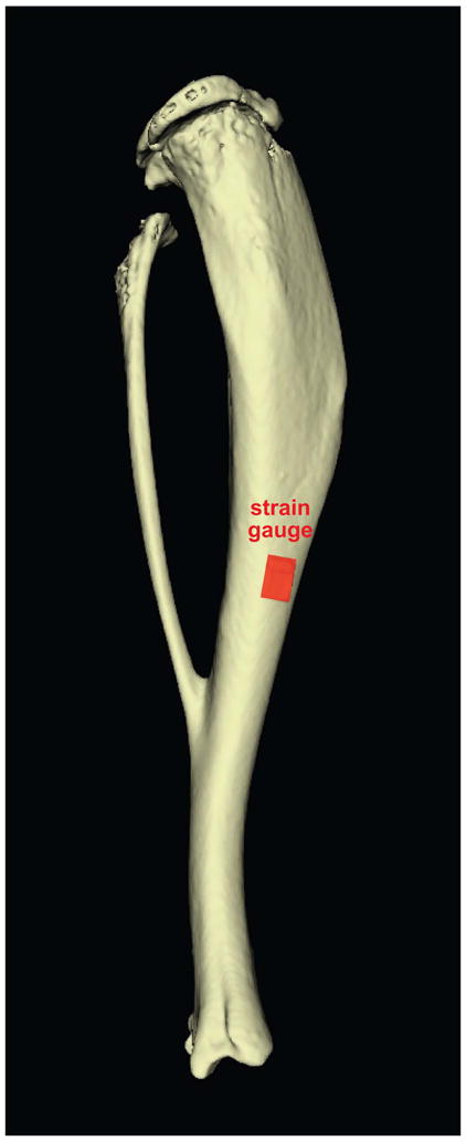
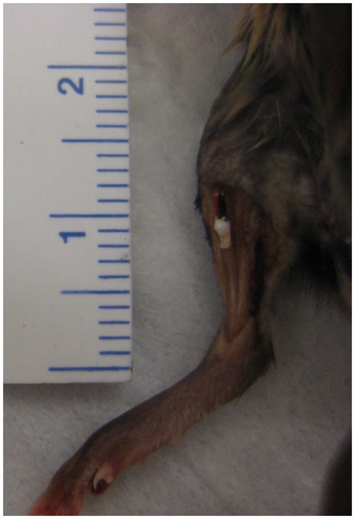
Proper strain gauge placement at the tibial midshaft. (A) Schematic showing strain gauge positioned at the middiaphysis of tibia. (B) Photograph of surgically-implanted gauge attached to surface of mouse tibia.

3.3 In Vivo Axial Tibial Loading Experimental Methods

3.3.1 Set Up and Preparation for In Vivo Axial Tibial Loading

1. Connect and power on all electronic signal conditioning components, including the loading device.

2. Open LabView loading program and insert proper loading parameters.

3. Zero the load cell. Check load offset by reading load when load cell is resting without any item positioned in the loading fixtures. Depending on your loading system, either enter the load offset in Newtons if an offset is entered directly or select the option to zero the load cell. The load from load cell should now read 0.0N (see ^{Note 11}).

4. Position a wooden rod in the loading device. Adjust and lock the horizontal position such that the rod is snug between the actuator and the load cell, but not so tight that the load cell is loaded beyond −1.0N.

5. Open and appropriately name the data file.

6. Run practice loading session with rod to warm up components and confirm the loading setup is working correctly and has no unforeseen issues.

3.3.2 Application of In Vivo Axial Tibial Loading

1. While rod is being loaded, turn on oxygen tank and isoflurane machine. Set oxygen flow to 1L/min and isoflurane flow to 2%, or whatever levels have been established in your protocol and approved by your Institutional Animal Care and Use Committee.

2. Place first mouse to be loaded into anesthesia chamber (Mouse A).

3. When Mouse A is asleep, remove Mouse A from chamber and apply eye ointment to each eye to maintain hydration during anesthesia, loading and recovery.

4. When test of wooden rod completes, promptly loosen fixtures and remove the rod.

5. Immediately check the load cell offset and adjust offset value if necessary so that the resting load cell reads 0.0N.

6. Remove Mouse A from the anesthesia chamber and place nose cone over nose.

7. Position Mouse A in the loading device, and lock the device so that the left tibia is snug. The left knee should be snug at the load cell cup and foot snug at the actuator (Figure 4). Once tibia is positioned and the device adjusted and locked, load cell should not read below −1.0N before loading begins or too much compressive preload is applied to the tibia (see ^{Note 12}).

8. Open a new data file and name the file appropriately to identify experiment, mouse, and date.

9. Begin the loading program when Mouse A’s breathing is slowed.

10. Monitor Mouse A during loading to check for continued slow breathing and unconsciousness (see ^{Note 13}).

11. Monitor the load cell and voltage outputs during the loading program (see ^{Note 14}).

12. When 2 to 3 minutes remain in the loading program, place the next mouse (Mouse B) into the isoflurane chamber (see ^{Note 15}).

13. When Mouse B is asleep, remove Mouse B from chamber and apply eye ointment to each eye to maintain hydration during anesthesia, loading and recovery.

14. Once loading program finishes, promptly unlock the loading device, remove Mouse A, and place on balance.

15. Check the load cell offset and adjust offset value if necessary so that the resting load cell reads 0.0N.

16. Record Mouse A body mass and place the animal into anesthesia recovery cage. Use one recovery cage per cage of mice. Once all mice from a single cage have been loaded, make sure all mice are awake and moving around before returning the animals to their original cage.

17. Position Mouse B into loading device, and adjust and lock the device so that left tibia is snug.

18. Repeat steps 7–17 for each subsequent mouse until all mice are loaded (Mouse B becomes Mouse A, and next mouse becomes Mouse B, etc.).

19. If a mouse loses >10% body mass over the course of an experiment, then wet food should be placed in the cage containing that mouse. If a mouse loses 20% body mass, that mouse should no longer be used for the experiment and should be appropriately euthanized.

20. Repeat procedure for each day that mice are to be loaded. Always load the same tibia for each mouse.

Figure 4.

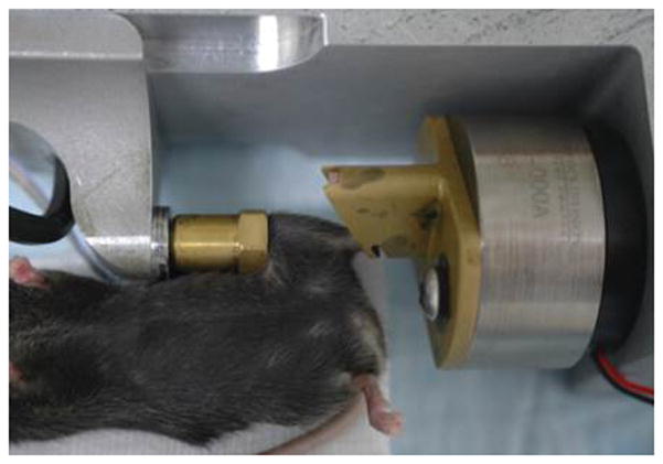
Mouse situated in loading device, ready for in vivo axial loading to be applied to the left tibia.

3.3.3 Clean up

1. Once final mouse is in recovery cage, turn off isoflurane and oxygen.

2. Close loading program software.

3. Turn off all electronic components.

3.4 Potential Outcome Measures

1. Cortical and cancellous morphology by microcomputed tomography

2. Gene expression by qRT-PCR

3. Dynamic histomorphometry using fluorochrome labeling

4. Protein localization by immunohistochemistry

5. Serum hormone assays by ELISA

6. Many others

Figure 5.

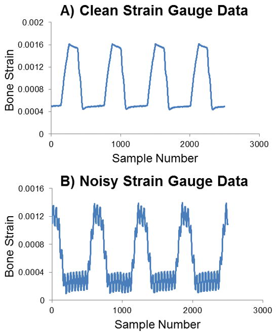
Sample strain gauge data. (A) Clean data with clear values, indicating proper gauge attachment. (B) Data with high frequency noise evident likely because the gauge is poorly attached or may be aligned off-axis. A new gauge should be used.

References

- 1.Turner CH, Akhter MP, Raab DM, Kimmel DB, Recker RR. A noninvasive, in vivo model for studying strain adaptive bone modeling. Bone. 1991;12(2):73–9. doi: 10.1016/8756-3282(91)90003-2. [DOI] [PubMed] [Google Scholar]
- 2.Lee KC, Maxwell A, Lanyon LE. Validation of a technique for studying functional adaptation of the mouse ulna in response to mechanical loading. Bone. 2002;31(3):407–12. doi: 10.1016/s8756-3282(02)00842-6. [DOI] [PubMed] [Google Scholar]
- 3.Fritton JC, Myers ER, Wright TM, van der Meulen MC. Loading induces site-specific increases in mineral content assessed by microcomputed tomography of the mouse tibia. Bone. 2005;36(6):1030–8. doi: 10.1016/j.bone.2005.02.013. [DOI] [PubMed] [Google Scholar]
- 4.Wallace JM, Rajachar RM, Allen MR, Bloomfield SA, Robey PG, Young MF, et al. Exercise-induced changes in the cortical bone of growing mice are bone- and gender-specific. Bone. 2007;40(4):1120–7. doi: 10.1016/j.bone.2006.12.002. [DOI] [PMC free article] [PubMed] [Google Scholar]
- 5.Prisby RD, Lafage-Proust MH, Malaval L, Belli A, Vico L. Effects of whole body vibration on the skeleton and other organ systems in man and animal models: What we know and what we need to know. Ageing Res Rev. 2008;7(4):319–29. doi: 10.1016/j.arr.2008.07.004. [DOI] [PubMed] [Google Scholar]
- 6.Iwamoto J, Takeda T, Sato Y. Effect of treadmill exercise on bone mass in female rats. Experimental animals/Japanese Association for Laboratory Animal Science. 2005;54(1):1–6. doi: 10.1538/expanim.54.1. [DOI] [PubMed] [Google Scholar]
- 7.De Souza RL, Matsuura M, Eckstein F, Rawlinson SC, Lanyon LE, Pitsillides AA. Non-invasive axial loading of mouse tibiae increases cortical bone formation and modifies trabecular organization: a new model to study cortical and cancellous compartments in a single loaded element. Bone. 2005;37(6):810–8. doi: 10.1016/j.bone.2005.07.022. [DOI] [PubMed] [Google Scholar]
- 8.Lynch ME, Main RP, Xu Q, Walsh DJ, Schaffler MB, Wright TM, et al. Cancellous bone adaptation to tibial compression is not sex dependent in growing mice. Journal of applied physiology. 2010;109(3):685–91. doi: 10.1152/japplphysiol.00210.2010. [DOI] [PMC free article] [PubMed] [Google Scholar]
- 9.Brodt MD, Silva MJ. Aged mice have enhanced endocortical response and normal periosteal response compared with young-adult mice following 1 week of axial tibial compression. Journal of bone and mineral research: the official journal of the American Society for Bone and Mineral Research. 2010;25(9):2006–15. doi: 10.1002/jbmr.96. [DOI] [PMC free article] [PubMed] [Google Scholar]
- 10.Sheng MH, Baylink DJ, Beamer WG, Donahue LR, Rosen CJ, Lau KH, et al. Histomorphometric studies show that bone formation and bone mineral apposition rates are greater in C3H/HeJ (high-density) than C57BL/6J (low-density) mice during growth. Bone. 1999;25(4):421–9. doi: 10.1016/s8756-3282(99)00184-2. [DOI] [PubMed] [Google Scholar]
- 11.Klein RF, Shea M, Gunness ME, Pelz GB, Belknap JK, Orwoll ES. Phenotypic characterization of mice bred for high and low peak bone mass. Journal of bone and mineral research: the official journal of the American Society for Bone and Mineral Research. 2001;16(1):63–71. doi: 10.1359/jbmr.2001.16.1.63. [DOI] [PubMed] [Google Scholar]
- 12.Wergedal JE, Sheng MH, Ackert-Bicknell CL, Beamer WG, Baylink DJ. Genetic variation in femur extrinsic strength in 29 different inbred strains of mice is dependent on variations in femur cross-sectional geometry and bone density. Bone. 2005;36(1):111–22. doi: 10.1016/j.bone.2004.09.012. [DOI] [PubMed] [Google Scholar]
- 13.Sabsovich I, Clark JD, Liao G, Peltz G, Lindsey DP, Jacobs CR, et al. Bone microstructure and its associated genetic variability in 12 inbred mouse strains: microCT study and in silico genome scan. Bone. 2008;42(2):439–51. doi: 10.1016/j.bone.2007.09.041. [DOI] [PMC free article] [PubMed] [Google Scholar]
- 14.Beamer WG, Donahue LR, Rosen CJ, Baylink DJ. Genetic variability in adult bone density among inbred strains of mice. Bone. 1996;18(5):397–403. doi: 10.1016/8756-3282(96)00047-6. [DOI] [PubMed] [Google Scholar]
- 15.Robling AG, Turner CH. Mechanotransduction in bone: genetic effects on mechanosensitivity in mice. Bone. 2002;31(5):562–9. doi: 10.1016/s8756-3282(02)00871-2. [DOI] [PubMed] [Google Scholar]
- 16.Saxon LK, Robling AG, Castillo AB, Mohan S, Turner CH. The skeletal responsiveness to mechanical loading is enhanced in mice with a null mutation in estrogen receptor-beta. Am J Physiol Endocrinol Metab. 2007;293(2):E484–91. doi: 10.1152/ajpendo.00189.2007. [DOI] [PubMed] [Google Scholar]
- 17.Nielsen RH, Christiansen C, Stolina M, Karsdal MA. Oestrogen exhibits type II collagen protective effects and attenuates collagen-induced arthritis in rats. Clin Exp Immunol. 2008;152(1):21–7. doi: 10.1111/j.1365-2249.2008.03594.x. [DOI] [PMC free article] [PubMed] [Google Scholar]
- 18.Glatt V, Canalis E, Stadmeyer L, Bouxsein ML. Age-related changes in trabecular architecture differ in female and male C57BL/6J mice. Journal of bone and mineral research: the official journal of the American Society for Bone and Mineral Research. 2007;22(8):1197–207. doi: 10.1359/jbmr.070507. [DOI] [PubMed] [Google Scholar]
- 19.Sample SJ, Collins RJ, Wilson AP, Racette MA, Behan M, Markel MD, et al. Systemic effects of ulna loading in male rats during functional adaptation. Journal of bone and mineral research: the official journal of the American Society for Bone and Mineral Research. 2010;25(9):2016–28. doi: 10.1002/jbmr.101. [DOI] [PMC free article] [PubMed] [Google Scholar]
- 20.Sugiyama T, Price JS, Lanyon LE. Functional adaptation to mechanical loading in both cortical and cancellous bone is controlled locally and is confined to the loaded bones. Bone. 2010;46(2):314–21. doi: 10.1016/j.bone.2009.08.054. [DOI] [PMC free article] [PubMed] [Google Scholar]
- 21.Srinivasan S, Ausk BJ, Poliachik SL, Warner SE, Richardson TS, Gross TS. Rest-inserted loading rapidly amplifies the response of bone to small increases in strain and load cycles. Journal of applied physiology. 2007;102(5):1945–52. doi: 10.1152/japplphysiol.00507.2006. [DOI] [PubMed] [Google Scholar]
- 22.Rubin CT, Lanyon LE. Dynamic strain similarity in vertebrates; an alternative to allometric limb bone scaling. Journal of theoretical biology. 1984;107(2):321–7. doi: 10.1016/s0022-5193(84)80031-4. [DOI] [PubMed] [Google Scholar]
- 23.Christiansen BA, Bayly PV, Silva MJ. Constrained tibial vibration in mice: a method for studying the effects of vibrational loading of bone. Journal of biomechanical engineering. 2008;130(4):044502. doi: 10.1115/1.2917435. [DOI] [PMC free article] [PubMed] [Google Scholar]