Benchmarking the Bethe–Salpeter Formalism on a Standard Organic Molecular Set

Abstract

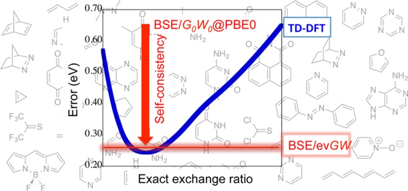
We perform benchmark calculations of the Bethe–Salpeter vertical excitation energies for the set of 28 molecules constituting the well-known Thiel’s set, complemented by a series of small molecules representative of the dye chemistry field. We show that Bethe–Salpeter calculations based on a molecular orbital energy spectrum obtained with non-self-consistent G₀W₀ calculations starting from semilocal DFT functionals dramatically underestimate the transition energies. Starting from the popular PBE0 hybrid functional significantly improves the results even though this leads to an average −0.59 eV redshift compared to reference calculations for Thiel’s set. It is shown, however, that a simple self-consistent scheme at the GW level, with an update of the quasiparticle energies, not only leads to a much better agreement with reference values, but also significantly reduces the impact of the starting DFT functional. On average, the Bethe–Salpeter scheme based on self-consistent GW calculations comes close to the best time-dependent DFT calculations with the PBE0 functional with a 0.98 correlation coefficient and a 0.18 (0.25) eV mean absolute deviation compared to TD-PBE0 (theoretical best estimates) with a tendency to be red-shifted. We also observe that TD-DFT and the standard adiabatic Bethe–Salpeter implementation may differ significantly for states implying a large multiple excitation character.

1. Introduction

The accurate calculation of excited-state properties remains one of the major challenges in theoretical chemistry. Among the popular approaches in the field, one finds several single-reference ab initio theories (e.g., time-dependent density functional theory (TD-DFT),^1,2 algebraic diagrammatic construction (ADC),³⁻⁵ equation-of-motion coupled cluster (EOM-CC),⁶⁻⁸ and symmetry adapted cluster configuration interaction (SAC–CI))^9,10 as well as multireference schemes (e.g., complete active space second-order perturbation theory (CAS-PT2)¹¹ and multi-reference configuration interaction (MR-CI)¹²). For a given problem, selecting the most efficient theory in terms of accuracy/effort ratio is not straightforward. This explains why, in recent years, there have been a wide variety of benchmark studies designed to evaluate the pros and cons of theoretical models in the framework of the determination of transition energies between electronic states. Among the sets of molecules used to perform these benchmarks, the set defined in 2008 by Thiel and his co-workers¹³⁻¹⁸ certainly remains the most widely investigated. It is constituted of 28 small representative molecules for which a large number of both singlet and triplet excited states have been computed on a frozen ground-state geometry obtained at the MP2/6-31G(d) level. In the original work, Schreiber et al. defined theoretical best estimates (TBE) for 104 singlet-singlet transitions as well as 63 singlet-triplet transitions.¹³ These TBE values were obtained either from reference literature values or from calculations performed with CAS-PT2, CC2, EOM-CCSD, and CC3 theories using the TZVP basis set.¹³ In 2010, Thiel and co-workers refined their own TBE using the aug-cc-pVTZ atomic basis set for both CAS-PT2¹⁸ and CC¹⁷ calculations. This led to the so-called TBE-2 estimates that are used as reference values here. These TBE and/or TBE-2 references were applied previously to benchmark semiempricial methods,^16,19,20 to compare the merits of iterative and non-iterative triples in third-order coupled-cluster estimations,¹⁵ to test several wave function schemes based on CC or ADC^21,22 as well as to appraise the performances of a large panel of TD-DFT approaches.^{14,19,23−35}

The present study is devoted to the evaluation of the merits of a family of techniques, namely, the many-body GW(36) and Bethe–Salpeter³⁷⁻³⁹ formalisms, for the study of the vertical transition energies in isolated organic molecules. These methodologies pertain to a specific group of many-body perturbation techniques that were not initially developed to tackle gas phase small- or medium-sized organic molecules. Indeed, the GW formalism was first used and tested to determine the electronic properties of the electronic jellium model³⁶ with first ab initio implementation performed for the accurate calculations of the band structure of simple semiconductors or insulators.^40,41 Concerning the Bethe–Salpeter Equation (BSE) formalism, it was initially derived in nuclear physics⁴² before being imported to the field of semiconductor physics at the semiempirical³⁷⁻³⁹ and later ab initio⁴³⁻⁴⁵ levels of theory to determine the optical properties of extended semiconductors, even though one of the first systems to be tested was the silane molecule.

Recently, the use of the GW and BSE formalisms for the calculation of the vertical excitation energies of gas phase organic molecules has become more widespread⁴⁶⁻⁶⁷ with the study of fullerenes, porphyrins, organic dyes, chromophores, and so forth. In particular, it was shown that one of the specific problems that the conventional TD-DFT formalism faces,^68,69 namely, difficulties in describing charge-transfer excitations, could be very efficiently and accurately cured by the BSE formalism. This has indeed been demonstrated in an increasing number of studies for both intramolecular^52,57,59 and intermolecular^54−56,62 charge-transfer excitations going from paradigmatic systems, such as dipeptides,^52,59 up to “real-life” donor–acceptor complexes, including fullerene/polymer aggregates of interest for photovoltaic applications.^55,56,62,66 In addition, the BSE approach was also found to be accurate for cyanine derivatives,^63,64 another family of compounds particularly challenging for TD-DFT.⁷⁰

We underline that to date, the results of GW and BSE calculations were generally validated through comparisons with experimental data with the limit that theoretical vertical excitation energies have often no experimental counterpart. Indeed, only in a few specific studies were comparisons of BSE with high-level quantum-chemistry techniques, such as CASPT2 or EOM-CC, performed.^52,59,63 The present paper thus aims to provide further assessment of the pros and cons of GW and BSE formalisms in the framework of molecular excitations using both Thiel’s reference values as well as an additional group of molecules relevant for dye chemistry.

2. Formalisms

The calculation of the optical excitations within the present GW/BSE scheme proceeds in two steps. One first performs a GW calculation that aims at providing accurate occupied/virtual electronic energy levels, labeled here below quasiparticle energies, including the ionization potential and electronic affinity in particular. In a second step, such output quasiparticle energies and the calculated screened-Coulomb potential W serve as an input to the Bethe–Salpeter equation that aims at providing neutral excitations by calculating the electron–hole interaction in particular. Our methodology section reflects this two-step scheme, presenting first the GW formalism and subsequently the Bethe–Salpeter equation.

2.1. Quasiparticle GW Formalism

The quasiparticle (QP) formalism, namely the mapping of the true many-body problem onto a single (quasi)particle framework, provides a formal background for obtaining QP energies, that is the electronic energy levels associated with occupied or virtual states as measured by direct and inverse photoemission. The associated eigenvalue equation reads

1

where we introduce a general Σ(r, r′; E) self-energy operator for the exchange and correlation contribution. The self-energy operator can be shown to be in general nonlocal, energy-dependent, and non-Hermitian, such that the corresponding eigenstates present an imaginary part interpreted as the lifetime of the quasiparticles with respect to electron–electron scattering.

Adopting Schwinger’s functional derivative approach to the many-electron problem,⁷¹ Hedin³⁶ showed that the self-energy can be given by a set of coupled equations relating self-consistently the one-body Green’s function, G, the screened-Coulomb potential, W, and the irreducible polarizability, P

2

3

4

5

6

where v(12) = v(r₁,r₂)δ(t₁ – t₂) is the bare Coulomb potential, ΔΓ(34; 2) = Γ(12; 3) – δ(12)δ(13), and Γ is the 3-body vertex correction. Such a set of equations can in principle be solved iteratively, starting from a zeroth-order system where the self-energy is zero, namely, the Hartree mean-field solution, yielding to first order: Γ(12; 3) = δ(12)δ(13). This simple approximation for the vertex correction yields the famous GW approximation for the self-energy,³⁶ which can be written in the energy representation as

7

8

9

10

where sgn is the sign function, and 0⁺ is a small positive infinitesimal. We have also introduced the zeroth-order one-body (ε_n,ϕ_n) mean-field eigenstates. P₀(r,r′; ω) is the irreducible polarizability (the f_i/j are the occupation factors) whereas W̃ = (W – v). The summations over occupied and empty states lead to an O(N⁴) scaling for GW calculations with respect to system size.

In practice, the mean-field starting point is never the Hartree solution but more traditionally DFT Kohn–Sham eigenstates, which in general represent the “best available” mean-field starting point. This leads to the standard “single-shot perturbative” G₀W₀ treatment, where the exchange-correlation contribution to the DFT Kohn–Sham eigenvalues is replaced by the GW self-energy operator expectation value onto the “frozen” Kohn–Sham DFT eigenstates

11

Such a formulation for the search of the quasiparticle energies is consistent with first-order perturbation theory, assuming in particular, as discussed here below, that the self-energy operator is diagonal in the Kohn–Sham basis.⁴⁰ Taking the local density approximation (LDA) to the exchange-correlation potential v^XC,DFT, for example, leads to the so-called G₀W₀@LDA scheme, the most common approach for GW calculations in solids.^40,41 Next, we explore the merits of the non-self-consistent G₀W₀@PBE and G₀W₀@PBE0 schemes, namely, single-shot G₀W₀ calculations aimed at correcting the Kohn–Sham PBE⁷² and PBE0^73,74 electronic energy levels.

As shown below and demonstrated in several recent studies,^58,75−85 the standard non-self-consistent G₀W₀@LDA or G₀W₀@PBE do not offer sufficient accuracy for isolated molecules, leading to underestimated ionization potential (IP) and HOMO–LUMO gaps. This can be ascribed to the fact that the starting point (zeroth-order) Kohn–Sham spectrum used to build the one-body Green’s function and screening potential W is too inaccurate when using the LDA or PBE exchange-correlation (XC) functionals, such that a simple “single-shot” perturbative treatment is not enough. Solutions to this problem may consist of finding the “best” (optimized) DFT starting point (e.g., using hybrid functionals with an “optimal” amount of exact exchange)^79,81 or starting with generalized Kohn–Sham formulations designed to provide accurate frontier orbital energies.^86,87

Another approach to improve the calculated quasiparticle energies is to use self-consistent GW calculations that offer the extra advantage of removing the starting point dependency and the need to optimize the Kohn–Sham functional for a given family of systems. By self-consistency, we mean that the corrected eigenvalues, and potentially eigenfunctions as well, are reinjected into the calculation of G, W, and Σ. Such an approach, in its various formulations, has been shown to significantly improve the accuracy of the GW formalism in many extended solids where single-shot G₀W₀ calculations are unsatisfying.^76,88−91 For molecular systems, much less data are available, but self-consistency has been demonstrated to improve on the standard non-self-consistent G₀W₀@PBE approach, though it remains unclear whether such success is systematic compared to single-shot G₀W₀ calculations starting from a hybrid functional including an “optimal” amount of exact exchange.^65,76,84,85 We note that such a “best starting point” for the single-shot G₀W₀ calculation was shown to be system dependent, because Hartree–Fock appears to be an excellent starting point for very small molecules,⁷⁵⁻⁷⁷ whereas PBE0 with ∼25% exact exchange would be much more accurate for medium-sized compounds.^80,82,92

We explore here a simple and computationally efficient self-consistent strategy that allows for the treatment of large systems. Namely, we explore a “partially” self-consistent scheme, where only the corrected eigenvalues are reinjected in the construction of the polarizability P and the Green’s function G. Once the updated self-energy is obtained, the quasiparticle eq 11 is solved again, yielding updated quasiparticle energies. Such a scheme was shown by several groups to provide vastly improved ionization potentials and HOMO–LUMO gaps^58,77,93 compared to G₀W₀@LDA or G₀W₀@PBE and subsequently to improve Bethe–Salpeter excitation energies.^56,58,77 The partial nature of the self-consistency is justified below by showing that “freezing” (not updating) the starting-point Kohn–Sham wave functions has a very limited impact on the final result. Such a simple partially self-consistent scheme is labeled evGW@PBE or evGW@PBE0 in the following when starting from PBE or PBE0 Kohn–Sham eigenstates, respectively.

2.2. The Bethe–Salpeter equation

We introduce here the BSE formalism in the language of linear response, which allows a direct connection with TD-DFT. We also highlight the basic approximations used in standard BSE calculations, approximations that one may have to question in light of the following results. We introduce the standard polarizability χ and its four-point generalization L, such that

12

where, for example, 1 = (r₁, t₁) is a space-time coordinate, n and V^ext are the standard charge density and external potential common with the language of TD-DFT, respectively, G is the one-body time-ordered Green’s function, and U^ext is a nonlocal external potential. Because the diagonal of G reduces to the charge density, it stems that χ(1, 2) = L(11, 22). This simple relation offers a fruitful direction to bridge linear response TD-DFT with Green’s function many-body perturbation theory.

For this to proceed further, taking the derivative of the relation relating G, G₀, and Σ (see above) with respect to the external potential U^ext leads to a Dyson-like self-consistent equation for L, such that

13

14

where v is the bare Coulomb potential. Such an equation resembles formally the fundamental TD-DFT equation for χ, replacing the charge density derivative of the XC potential by the (∂Σ/∂G) four-point generalized “kernel”. Although this equation is exact, one now proceeds with approximations for the self-energy operator. The spirit of the BSE formalism in condensed matter physics is to use the GW approximation for the self-energy Σ with the obvious derivation

This is consistent with the use of the GW approximation for calculating the occupied and virtual energy levels that will be used to build the optical excitations. It is assumed that in the derivative of Σ^GW, one may neglect the (∂W/∂G) variations. Such an approximation has been used since the very early days of the Bethe–Salpeter formalism applied to condensed-matter physics with a justification that can be traced back to the original paper by Sham and Rice.³⁷ The proposed argument is that (δW/δG) is a vertex correction that can be neglected consistently with the approximation leading to the GW formalism, even though no explicit numerical evaluation of such a term can be found in the literature for real systems. As a result, the four-point kernel K reduces to

15

Finally, due to computational cost, the standard implementation of the BSE formalism assumes a static (frequency-independent) approximation for the screened Coulomb potential, namely, W(56) = W(r₅,r₆)δ(t₅-t₆). Such an approximation is equivalent to assuming an adiabatic kernel within the TD-DFT framework. It is known to significantly affect the calculations of transitions with multiple-excitation character because a static kernel is expected to shift the energy of the single-electron transitions contained in the independent-electron susceptibility without creating new poles associated with multiple excitations.^94,95 It is worth emphasizing at this stage however that the “full” (dynamical) BSE formalism exists on paper and has been explored under various approximations,^96,97 but the cost associated with such an extension impedes its systematic application to large molecules.

As a final step, we express the L operator in transition space between occupied and virtual orbitals

16

17

where we have used the fact that a static screened-exchange W leads to a “four-point one-time” only L(t–t′) operator, that is a one-frequency L(ω) functional in the energy domain. Such a treatment leads to a formulation that resembles the so-called Casida’s equation to TD-DFT,² and the optical excitations can be obtained as the eigenvalues of the Bethe–Salpeter eigenvalue problem that reads in transition space

18

where the indexes (i,j) and (a,b) indicate the occupied and virtual orbitals, and (r_e,r_h) indicate the electron and hole positions, respectively. In this block notation, the vector [ϕ_a(r_e) ϕ_i(r_h)] represents all excitations (e.g., note that ϕ_a(r_e) means that an electron is put into a virtual orbital), whereas the vector [ϕ_i(r_e) ϕ_a(r_h)] represents all de-excitations. As such, R (R*) describes the resonant coupling between electron–hole excitations (de-excitations), and the off-diagonal block C and C* account for nonresonant coupling between excitations and de-excitations. The TD-DFT and BSE resonant parts can be directly compared, and we write here the Bethe–Salpeter formulation in the approximation listed above

19

We use the notation ⟨...⟩ for the ∫∫ drdr′ double integral. The middle (last) line gathers terms with occupied and virtual orbitals taken at different (identical) integration variables with the important consequence that the W matrix elements do not vanish for spatially separated electrons and holes, leading in particular to the correct Mulliken limit for charge-transfer excitations. For isolated systems, the wave functions can be taken to be real. The resonant terms have been written above for singlet excitations that will be the focus of the present study. Obtaining the Bethe–Salpeter vertical excitation energies comes thus at the same price as the standard TD-DFT within Casida’s formulation, and we use recursive techniques to obtain the lowest desired excitation energies. The eigenvectors solution of the Bethe–Salpeter equation yields the electron–hole two-body wave functions ψ^eh(r_e, r_h) with the standard interpretation that it represents the amplitude of probability of finding an electron and a hole in (r_e, r_h).

2.3. Computational Details

For the molecules of Thiel’s set, we have used the MP2/6-31G(d) geometries supplied in ref (13) and selected the most refined best estimates, the so-called TBE-2 (see Introduction), as reference values. Our GW calculations are performed at the all-electron level with the aug-cc-pVTZ correlation consistent atomic basis set^98,99 using the Fiesta code,^54,77 implementing resolution-of-the-identity (RI) techniques. The input Kohn–Sham eigenstates are generated with the NWChem package.¹⁰⁰ The implemented RI or Coulomb fitting technique expresses four-center integrals in terms of three-center integrals combined with the aug-cc-pVTZ-RI basis by Weigend and co-workers.¹⁰¹ We provide in the Supporting Information (SI) a comparison with aug-cc-pVQZ calculations for butadiene, benzene, benzoquinone, and adenine, namely, one representative of each chemical family in Thiel’s set.

All virtual states are included in the construction of both the polarizability P and the self-energy Σ. The energy integration required to calculate the correlation self-energy is achieved by contour deformation techniques and does not involve any plasmon-pole approximation. Because the correlation contribution to the self-energy Σ(E^QP) must be calculated at the targeted (unknown) E^QP quasiparticle energy, we calculate Σ(E) on a fine energy grid to solve eq 11. We do not advocate the standard linear extrapolation from the value of the self-energy at the input Kohn–Sham DFT energy, which may lead to sizable errors. We typically correct at the GW level all occupied valence states and the same number of virtual states above the gap, even though convergency tests show that for medium size molecules, such as naphthalene or nucleobase, correcting only 10 to 20 occupied and virtual states is enough. For the BSE calculations, performed with the Fiesta code, all valence and virtual states are included in the electron–hole product space within which the electronic excitations are built. We go beyond the Tamm–Dancoff approximation in the present study, namely, we mix resonant and nonresonant contributions.

To identify the transitions, we ran TD-PBE0 calculations with Gaussian09¹⁰² and CC2 calculations with Turbomole,¹⁰³ both using the aug-cc-pVTZ atomic basis set. Results (orbital compositions, oscillator strengths, symmetry, etc.) were compared to previous calculations of Thiel’s group^17,18 to establish the correct nature of the excited states. As noted in the study by Thiel and co-workers devoted to basis size effects,¹⁷ the identification of transitions generated by two different approaches is more complicated with the aug-cc-pVTZ atomic basis set, as compared with the diffuse-less TZVP atomic basis set, which yields less excited states. We therefore followed ref (17) and discarded the few states located at high energy for which the correspondence between TD-PBE0/CC2 and BSE data were not convincing. As a result, we keep 90 transitions for which the identification between the various single-shot and self-consistent GW/BSE could be safely performed with respect to both TD-PBE0 and TBE-2. This represents 86% of the 104 transitions for which TBE-2 data are available. Concerning comparisons between BSE and TD-PBE0, our statistics are based on 157 transitions because with the aug-cc-pVTZ basis, several transitions intercalate between the excitations listed in the original TZVP study.¹³ We underline that PBE0, which contains 25% of exact exchange,^73,74 was selected because it was shown to be particularly accurate for Thiel’s set of compounds.²⁴ The selection of another exchange-correlation functional for the TD-DFT calculations could lead to strongly different estimates, a topic discussed in detail previously and summarized below in section 3.2.5.

For the set of molecules treated in section 3.3, we have first optimized the ground-state geometries at the MP2/aug-cc-pVTZ level using Gaussian 09,¹⁰² applying a tight convergence threshold (residual rms force <1.0 × 10^–5 au). Next, theoretical best estimates were obtained from CC2, CCSD, CCSDR(3), and CC3 calculations using both aug-cc-pVDZ and aug-cc-pVTZ (see section 3.3 for details). These EOM-CC calculations were obtained with the Dalton code.¹⁰⁴ The TD-PBE0 and BSE energies have been obtained with the aug-cc-pVTZ atomic basis set as explained above.

3. Results

3.1. Importance of Self-Consistency: The Case of the Nucleobase

To introduce our methodology and the calculations that are carried out below, we first address the specific case of the nucleobase, commenting on both the electronic and optical properties. As emphasized in the Introduction, the Bethe–Salpeter calculation of the optical properties starts from a GW description of the occupied and virtual electronic energy levels. Even though the present paper focuses on optical excitations, the availability of CAS-PT2 and EOM-CCSD(T) vertical ionization potential (IP)¹⁰⁵ of the nucleobase offers an excellent position to start illustrating the importance of self-consistency at the GW level.

We compare in Table 1 the IP of the nucleobases calculated non-self-consistently starting from PBE and PBE0 Kohn–Sham eigenstates, using the G₀W₀@PBE and G₀W₀@PBE0 approaches, to the IP obtained through updated quasiparticle energies labeled evGW@PBE and evGW@PBE0. For the “standard” G₀W₀@PBE technique, it clearly appears that the IP are dramatically too small, leading to a mean absolute error (MAE) of 0.51 eV compared to the CCSD(T) benchmarks. Such a large underestimation of the G₀W₀ IP when starting from (semi)local functional Kohn–Sham eigenstates was previously reported for various sets of compounds.^76,77,82 This originates in the too inaccurate initial Kohn–Sham spectrum. Subsequently, several solutions have been explored.

Table 1. Theoretical GW Ionization Potentials (IP) and BSE Lowest Singlet Excitation Energies (S₁) for the Nucleobase Obtained with the aug-cc-pVTZ Atomic Basis Set^a.

	G0W0@		ev(G)W0	evGW@
	PBE	PBE0	@PBE	PBE	PBE0	ref values	ref
Ionization Potential (IP)
Cyt	8.16 (8.18)	8.56	8.59	8.90	8.90	8.73/8.76	(105)
Thy	8.60 (8.63)	8.95	8.88	9.18	9.23	9.07/9.04	(105)
Ura	8.98 (8.99)	9.35	9.32	9.60	9.65	9.42/9.43	(105)
Ade	7.84 (7.99)	8.11	8.11	8.30	8.33	8.37/8.40	(105)
MAE	0.51	0.16	0.18	0.14	0.15
Lowest Singlet Excitation S1
Cyt	3.54	4.12	4.11	4.53	4.57	4.66	(18)
Thy	3.47	4.20	4.42	4.79	4.72	4.82	(18)
Ura	3.44	4.16	4.40	4.75	4.70	5.00	(18)
Ade	4.08	4.59	4.54	4.83	4.93	5.12	(18)
MAE	1.27	0.63	0.53	0.17	0.17

^aAll values are in eV. The GW IP data are compared to the CAS-PT2/CCSD(T) results of ref (105). The mean absolute errors take the CCSD(T) value as the reference for the ionization potential, and the TBE-2 theoretical estimate of ref (18) for the S₁ transition energy. The G₀W₀@PBE value in parentheses refers to the “planewave/periodic boundary condition” calculations by Qian et al. in ref (106). The mean absolute error (MAE) are given for both IP and transition energies.

A first solution consists of optimizing the Kohn–Sham starting point⁸¹ to provide a much better zeroth-order solution to proceed with the G₀W₀ perturbative approach. In particular, the use of the global hybrid PBE0 functional has already been shown to provide very good results for a few systems.^76,82,92 This is indeed what we observe in Table 1 with the MAE reduced to 0.16 eV with values approaching the CCSD(T) reference from below. Our study confirms previous reports that the IPs are described much better when using the PBE0 functional to define the initial eigenstates. We show below that this conclusion does not necessarily apply to optical properties.

Though excellent frontier orbital energies can be obtained with optimally tuned functionals,^86,87,93 the interest of the self-consistent approach can be illustrated for the IP by comparing evGW@PBE and evGW@PBE0 data to the reference calculations. The agreement is excellent with MAEs of 0.14 and 0.15 eV, respectively. The good agreement between evGW@LDA and CCSD(T) calculations for several states around the gap was also illustrated in ref (78). A second important feature is that the partially self-consistent evGW@PBE and evGW@PBE0 techniques led to extremely similar results. In other words, the “starting point” dependency is dramatically reduced, and the need to optimize the XC functional for a given class of compounds can be bypassed. This comes at a somehow higher computational cost, however, because ∼5 iterations are necessary to reach convergence. As emphasized above in section 2.1, the remaining slight discrepancy lies in the difference between the PBE and PBE0 Kohn–Sham wave functions that are not self-consistently updated in the partial self-consistent scheme adopted here.

We now turn to the transitions of the lowest lying singlet S₁ states, again comparing BSE calculations starting from G₀W₀@PBE or G₀W₀@PBE0 eigenstates to BSE results starting from evGW@PBE and evGW@PBE0 calculations. As above, we observe that the BSE/G₀W₀@PBE data provide very poor results, leading to dramatically too small excitation energies with an MAE of 1.27 eV. The BSE/G₀W₀@PBE0 estimates are more accurate though the deviations remain large (MAE of 0.63 eV). The two self-consistent approaches, namely BSE/evGW@PBE and BSE/evGW@PBE0, yield a much better agreement with the reference data and a strongly reduced starting point dependency. This is why we adopt this self-consistent scheme in the following, systematically starting both from PBE and PBE0 eigenstates to check for the consistency of this approach. We also provide the popular BSE/G₀W₀@PBE0 results for the sake of comparison.

To conclude, let us consider the ev(G)W₀ approach, namely, an intermediate scheme where only the Green’s function G is self-consistently updated while the screened-Coulomb potential is kept frozen. Such an approach was advocated in solids^107,108 and further presents the advantage that the polarizability matrix does not need to be recalculated. Taking as a starting point the PBE XC functional for which self-consistency is clearly needed, the ev(G)W₀ approach is found to significantly improve both the IP and S₁ estimates, even though a significant residual error remains for the latter. Further, as shown in ref (109) for the azabenzene family, a significant starting point dependency remains in this intermediate scheme.

3.2. Thiel’s Set

We now turn to comparisons with the TBE-2 values of Thiel’s set. The description of the molecules can be found in Figure 1 of ref (13), which also provides the atomic positions in the associated Supporting Information. We divide our analysis in different subsets composed of compounds belonging to the same chemical family. For all sets, we analyze the Bethe–Salpeter data based on the non-self-consistent G₀W₀@PBE0 approach and on the self-consistent evGW@PBE and evGW@PBE0 schemes. Full data are provided in the SI. These excitation energies are compared to TD-PBE0/aug-cc-pVTZ results as well as to the TBE-2 theoretical best estimates when available. The selection of PBE0 to perform the TD-DFT reference calculations is justified by a previous benchmark of TD-DFT performed for the Thiel set.²⁴ In that work, it was shown that among the 28 XC functionals considered, TD-PBE0 yields the smallest MAE (0.24 eV) and the largest correlation or regression coefficient (r = 0.95) using Thiel’s TBE as reference. Other XC functionals might deliver significantly larger deviations, for example, an MAE of 0.53 eV with a nearly systematic underestimation of the TBE values for TD-PBE and an MAE of 0.31 eV with a tendency toward overestimation for CAM-B3LYP.

3.2.1. Unsaturated Aliphatic Hydrocarbons

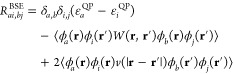
For the unsaturated aliphatic hydrocarbons, the BSE and TD-PBE0 transitions have been considered up to the last transition for which the TBE-2 values have been determined, leading to a total of 29 transitions. The excitation energies, oscillator strengths, and main characteristics of the states are given in the SI. Our data are compiled in Figure 1, where statistics are provided. Confirming our previous insight with the lowest lying excitations for the nucleobase family, we found an excellent correlation between the evGW@PBE and evGW@PBE0 energies with a correlation coefficient r of 0.993 and an MAE of 0.09 eV (see Figure 1a). The close agreement between these two data sets shows that the dependency on the starting point DFT functional is dramatically reduced compared to standard non self-consistent BSE approaches, indicating that the discrepancies between the PBE and PBE0 wave functions that are kept frozen in our approach do not significantly impact the excitation energies.

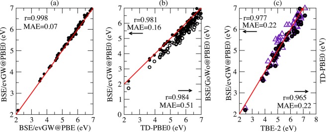
Figure 1.

Unsaturated aliphatic hydrocarbons: plot of (a) BSE/evGW@PBE0 (closed circles) vs BSE/evGW@PBE, (b) BSE/evGW@PBE0 and BSE/G₀W₀@PBE0 (open circles) vs TD-PBE0, and (c) BSE/evGW@PBE0 and TD-PBE0 (violet triangle) vs best theoretical estimates (TBE-2) from ref (18). Energies are in eV. The regression coefficients r and MAE (in eV) are indicated. The red lines are the first diagonals as a visual reference. The red arrow in (b) and the red arrow “1” in (c) indicate the 2¹A_g transition in octatetraene, and the red arrow “2” in (c) indicates the 2¹A_g transition in hexatriene.

The comparison between our BSE/evGW@PBE0 approach (closed circles in Figure 1b,c) and the TD-PBE0 data also reveals excellent correlation with a regression coefficient r of 0.984 and a small MAE of 0.11 eV. The largest deviation of 0.51 eV (indicated by a red arrow in Figure 1b) is associated with the 2¹A_g (π–π*) transition in octatetraene. This is the transition with the maximal weight of contributions from the multiple excitations¹¹⁰ in the EOM-CC calculations of ref (13). We comment on these specific states below.

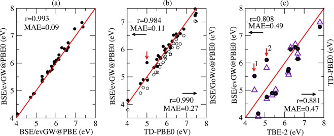
The non-self-consistent BSE/G₀W₀@PBE0 approach (open circles in Figure 1b) yields lower transition energies than both the BSE/evGW@PBE0 and TD-PBE0 data with a mean absolute deviation of 0.27 eV compared to TD-PBE0. This conclusion is also confirmed by the histogram in Figure 2 showing the distribution of BSE transitions as a function of the deviation with respect to TD-PBE0. Clearly, BSE/G₀W₀@PBE0 provides smaller values than TD-PBE0, whereas BSE/evGW@PBE0 excitation energies are distributed around the TD-PBE0 values.

Figure 2.

Histograms showing the number of transitions as a function of the difference in energy (eV) with respect to TD-PBE0 data for the (a) BSE/G₀W₀@PBE0 and (b) BSE/eGW@PBE0 results. The red arrow indicates the 2¹A_g transition in octatetraene.

We compare our data to TBE-2 in Figure 1c. The discrepancies between BSE/evGW@PBE0 or TD-PBE0 with the TBE-2 references are clearly larger than in the previous graphs with correlation coefficients reduced to approximately 0.88 and 0.81 for the TD-PBE0 and BSE/evGW@PBE0 approaches, respectively, and an MAE of ∼0.48 eV for both methods. Besides the case of the 2¹A_g transition in octatetraene (red arrow “1” in Figure 1c), where the BSE/evGW@PBE0 is ∼1 eV too high in energy and clearly worse than the TD-PBE0 value, both approaches perform similarly compared to reference wave function calculations. This is a first indication that BSE/evGW@PBE0 and TD-PBE0 deviate significantly only for transitions with multiple-excitation character despite the adiabatic nature of the present TD-DFT and BSE implementations. EOM-CC calculations that include an explicit operator to describe these multiple excitations, namely, excitations involving the simultaneous promotion of more than one electron in the virtual states, are expected to deliver a more accurate picture of excited states presenting such character.

To start our discussion on this issue, we underline that for the 2¹A_g transition in hexatriene, the aug-cc-pVTZ CC2 and CCSDR(3) values are 6.43 and 6.09 eV, respectively,¹⁷ which are 1.34 and 1.0 eV higher than the 5.09 eV TBE-2 value. For this transition, the BSE/evGW@PBE0 (6.11 eV) results are more accurate than CC2 and are very close to the CCSDR(3) values. Similarly, for the 2¹A_g transition in octatetraene, the CC2/aug-cc-pVTZ excitation energy is 5.74 eV,¹⁷ which is 1.27 eV above its TBE-2 counterpart (4.47 eV), whereas TD-PBE0 and BSE/evGW@PBE0 approaches overshoot the TBE-2 values by 0.53 and 1.05 eV, respectively. In other words, the self-consistent BSE approach yield results that are closer to the reference CC calculations than TD-PBE0 for the states with a strong multiple-excitation character. Below, we will see other examples confirming this observation.

3.2.2. Aromatic Hydrocarbons and Heterocycles

We now consider the cyclic molecules contained in Thiel’s set, namely 11 molecules for a total of 70 transitions. We follow the same procedure as above, starting by confirming the good agreement between BSE/evGW@PBE and BSE/evGW@PBE0 figures to validate the present self-consistent scheme. Indeed, as shown in Figure 3a, the two sets of data agree with a large linear regression coefficient (r = 0.998) and a small MAE (0.07 eV).

Figure 3.

Aromatic compounds: plot of (a) BSE/evGW@PBE0 (closed circles) vs BSE/evGW@PBE, (b) BSE/evGW@PBE0 and BSE/G₀W₀@PBE0 (open circles) vs TD-PBE0, and (c) BSE/evGW@PBE0 and TD-PBE0 (violet triangle) vs best theoretical estimates (TBE-2) from ref (18). See Figure 1 caption for more details.

The agreement between BSE/evGW@PBE0 (closed circles in Figure 3b) and TD-PBE0 is overall excellent with a regression coefficient of 0.9815 and an MAE of 0.16 eV. In contrast, the non-self-consistent BSE/G₀W₀@PBE0 scheme yields much larger deviations compared to TD-PBE0 (MAE of 0.51 eV). A comparison of the self-consistent BSE/evGW@PBE0 and TD-PBE0 results with the theoretical best estimates (TBE-2) leads to the same MAE of 0.22 eV for both methods (see Figure 3c) with a regression coefficient slightly in favor of the former theory. The analysis of the histograms showing the deviations of TD-PBE0 (Figure 4a) and BSE/evGW@PBE0 (Figure 4b) with respect to TBE-2 indicates that although both peaked at approximately −0.15 eV, the TD-PBE0 (BSE) error distribution tends to have a stronger weight at higher (lower) energies.

Figure 4.

Histograms showing the number of transitions as a function of the difference in energy (eV) with respect to the theoretical TBE-2 best estimates data for (a) the TD-PBE0 and (b) BSE/evGW@PBE0 results for the derivatives of Figure 3. The dashed box in (a) indicates the set of high lying TD-PBE0 excitations showing a large multiple-excitation character.

The transitions for which TD-PBE0 overestimates the TBE-2 values by more than 0.3 eV are collected in Table 2, which provides TD-PBE0, BSE/evGW@PBE0, and CC2 errors with respect to the TBE-2 reference values. As can be seen from the percent T₁ values taken from ref (13), all of these transitions imply a quite large weight (>10%) of multiple excitations.¹¹⁰ There is, as expected, a strong correlation between a large multiexcitation character and the failure of TD-PBE0. This is related to the adiabaticity of the TD-DFT kernel that does not allow for the capture of multiple excitations.^94,95 Even though the present BSE implementation relies as well on a static (adiabatic) approximation, the BSE excitation energies do not undergo such a severe blueshift, confirming that BSE and TD-PBE0 behave differently for these states. To be thorough, we have repeated our calculations with the cc-pVTZ atomic basis set to check if possible intruder states could bias our analysis. The difference between TD-PBE0 and BSE/evGW@PBE0 reduced from 0.55 to 0.51 eV for the 1¹B_2u state of tetrazine, which shows the largest discrepancy between the two approaches. The second largest deviation (0.51 eV for the 1¹B_2u state of pyrazine) is reduced to 0.41 eV. In short, removal of the diffuse orbitals does not lead to the disappearance of the differences between TD-PBE0 and BSE/evGW@PBE0.

Table 2. Error with Respect to the Theoretical Best Estimate for Selected Transitions with Multiple Character As Indicated by the T₁ Diagnostic Taken from Thiel’s Study¹³ by Comparing the Present TD-PBE0 and BSE/evGW@PBE0 Calculations to the CC2 Estimates of Ref (17)^a.

			error vs TBE-2
		CC3 (%T1)	TD-PBE0	BSE	CC2
pyridine	11B2	85.9	0.68	0.23	0.41
tetrazine	11B2u	84.6	0.52	–0.03	0.08
triazine	11A2′	85.1	0.49	0.05	0.09
pyridazine	21A1	85.2	0.44	–0.04	0.12
pyrimidine	11B2	85.7	0.44	–0.03	0.12
pyrazine	11B2u	86.2	0.40	–0.11	0.10
benzene	11B2u	85.8	0.37	–0.04	0.14
naphthalene	21Ag	82.2	0.31	–0.06	0.11

^aAll errors are in eV and have been determined with the aug-cc-pVTZ atomic basis set.

Whereas the BSE excitation energies were larger than that of TDPBE0 for the 2¹A_g transitions in hexatriene and octatetraene, showing a significant multiexcitation character as well, the BSE transition energies here stand significantly below their TD-PBE0 counterpart in much better agreement with the TBE-2 reference. It is certainly too early to provide a definitive explanation for such a behavior, but we similarly observe that CC2 energies were significantly larger than that of TD-PBE0 for the 2¹A_g transitions in hexatriene and octatetraene, whereas here, on the contrary, both CC2 and BSE data stand at lower energy, much closer to the TBE-2 references. Again, even though “adiabatic” in its present implementation, the BSE formalism yields transition energies closer to CC data for transitions showing multiple-excitation character, the BSE energies being even closer to TBE-2 values than their CC2 counterparts.

3.2.3. Aldehydes, Ketones, and Amides

The third family of molecules in Thiel’s reference set is composed of representatives of the aldehyde, ketone and amide families. We have encountered specific problems for the amide derivatives: using the aug-cc-pVTZ atomic basis set anomalously yields large instability for the lowest lying 1¹A₂′′ (n–π*) excitations within the GW/BSE formalism. As can be seen in Table 3, this problem is related to the presence of diffuse orbitals because BSE and TD-PBE0 agree extremely well at the cc-pVTZ level. Further, the augmentation of the atomic basis set significantly increases the discrepancies between BSE/evGW@PBE and BSE/evGW@PBE0 to values as large as 0.5 eV, which largely exceed the typical 0.1 eV deviation found for most molecules. This instability originates in the GW correction to the final state of the transition, namely, the (LUMO+1) virtual state at the aug-cc-pVTZ level, which is lowered by more than 1 eV when switching to the augmented basis. For the sake of comparison, the HOMO is lowered by only ∼0.1 eV. Such an instability is tentatively attributed to the intercalation below the cc-pVTZ LUMO of a diffuse (virtual) orbital upon basis augmentation, which might not be well described (delocalized enough) with a simple augmentation.¹¹¹ Consequently, below, rather than discarding the three amide molecules, we used the BSE/cc-pVTZ values in our statistical analysis comparing them to the corresponding TD-PBE0/cc-pVTZ values.

Table 3. Amide 1¹A₂′′ (n–π*) excitations with three atomic basis sets. TD-PBE0 value and, in parentheses, the difference between the TD-PBE0 and BSE/evGW@PBE0 values.

atomic basis set	formamide	acetamine	propanamide
aug-cc-pVTZ	5.51 (0.29)	5.54 (0.98)	5.57 (0.99)
cc-pVTZ	5.61 (0.03)	5.64 (0.08)	5.67 (0.12)
cc-pVDZ	5.64 (−0.06)	5.65 (0.04)	5.70 (0.06)

Under such a restriction, we recover the behavior observed for the previous families, namely, that the BSE/evGW@PBE and BSE/evGW@PBE0 transition energies come in very good agreement with each other with a correlation coefficient close to 1 and an MAE of 0.10 eV (see Figure 5a). It is obvious from Figure 5b that inclusion of self-consistency increases the transition energies, which is consistent with the previous findings. The non-self-consistent BSE/G₀W₀@PBE0 data underestimates the TD-PBE0 energies with an MAE of 0.37 eV and a mean signed error (MSE) of −0.35 eV. Contrary to other families, we note here that the self-consistent BSE/evGW@PBE0 tends to overestimate the TD-PBE0 energies with an MAE of 0.30 eV and an MSE of +0.23 eV.

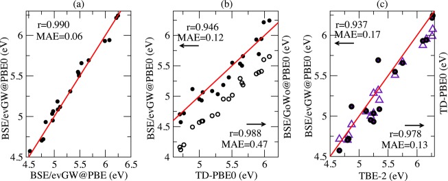
Figure 5.

Aldehydes, ketones, and amides: plot of (a) BSE/evGW@PBE0 (closed circles) vs BSE/evGW@PBE, (b) BSE/evGW@PBE0 and BSE/G₀W₀@PBE0 (open circles) vs TD-PBE0, and (c) BSE/evGW@PBE0 and TD-PBE0 (violet triangle) vs best theoretical estimates (TBE-2) from ref (18). See Figure 1 caption for more details.

The advantage of self-consistency becomes clear, however, when comparing with the TBE-2 data, because the BSE/G₀W₀@PBE0 approach leads to 0.63 eV MAE discrepancy, which is reduced to 0.24 eV with BSE/evGW@PBE0. Similarly, the mean signed error with respect to TBE-2 reduces from −0.63 to −0.07 eV upon switching on the self-consistency. A comparison of BSE/evGW@PBE0 and TD-PBE0 values to their TBE-2 counterparts is provided in Figure 5c. The two approaches provide rather similar trends with a nevertheless smaller MAE for the TD-PBE0 approach (0.18 eV) than for the BSE model (0.24 eV). The TD-PBE0 r is also larger than its BSE counterpart. The analysis of the histograms showing the deviations of these two theories (Figure 6) confirms that TD-PBE0 provides less disperse estimates but with a stronger tendency toward underestimation than BSE. Indeed, the MSE attains −0.16 eV with TD-PBE0 but only −0.07 eV with BSE/evGW@PBE0.

Figure 6.

Histograms showing the number of transitions as a function of the difference in energy (eV) with respect to the theoretical TBE-2 best estimates data for the (a) TD-PBE0 and (b) BSE/evGW@PBE0 results for the compounds in Figure 5.

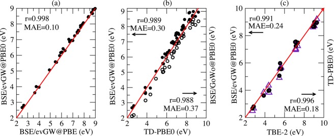
3.2.4. Nucleobase

We conclude the exploration of Thiel’s set of families by returning to the nucleobase case, now exploring higher energy excitations. We provide comparisons for the 20 states for which TBE-2 values are available in Figure 7. Following the same comparison sequence as before, we first find that the BSE/evGW@PBE0 and BSE/evGW@PBE data are extremely similar to a mean absolute deviation of 0.06 eV with a very large linear regression coefficient r of 0.990. Next, the analysis of Figure 7b confirms that the non-self-consistent BSE/G₀W₀@PBE0 scheme underestimates the TD-PBE0 data by an average of 0.47 eV, whereas the self-consistent BSE/evG₀W₀@PBE0 approach gives a much smaller difference with an MAE of 0.12 eV and an MSE of −0.02 eV, indicating a trifling redshift compared to TD-PBE0. Finally, the comparison with TBE-2 in Figure 7c indicates that both BSE/evGW@PBE0 and TD-PBE0 provide rather accurate estimates with MAEs of 0.17 and 0.13 eV, respectively, and a linear regression coefficient that is larger for TD-PBE0. The BSE/evGW@PBE0 statistics are mainly impaired by two outliers compared to TBE-2, and these correspond to the 1¹A″ et 2¹A″ states of cytosine. It is for this latter state that the identification between BSE and TD-PBE0 was less obvious. In short, in the absence of excitations showing clear multiple character, the TD-DFT and BSE formalisms perform well, provided that self-consistency is accounted for in the latter.

Figure 7.

Nucleobases: plot of (a) BSE/evGW@PBE0 (closed circles) vs BSE/evGW@PBE, (b) BSE/evGW@PBE0 and BSE/G₀W₀@PBE0 (open circles) vs TD-PBE0, and (c) BSE/evGW@PBE0 and TD-PBE0 (violet triangle) vs best theoretical estimates (TBE-2) from ref (16). See Figure 1 caption for more details.

3.2.5. Statistics for the Full Set

For the full set of excited-states, we obtained a deviation between the BSE/evGW@PBE and BSE/evGW@PBE0 estimates limited to 0.08 eV with a very large correlation coefficient (0.9979). Similar to that for the individual chemical families analyzed above, the use of self-consistency not only decreases the dependence to the original Kohn–Sham eigenvalues but also drastically diminishes the discrepancy with TD-PBE0 that amounts to 0.18 eV for BSE/evGW@PBE0 compared with 0.44 eV for BSE/G₀W₀@PBE0. In Table 4 and Figure 8, we provide a statistical analysis considering all families. Clearly, the non-self-consistent BSE/G₀W₀@PBE scheme is very unsatisfying with a large MAE (0.615 eV) and a quasi-systematic underestimation of the reference transition energies. Nevertheless, this popular approach provides the trends accurately (r = 0.980). The results obtained with the self-consistent BSE and TD-PBE0 approaches are rather similar with MAEs of 0.253 and 0.232 eV, respectively, and equivalent correlation coefficients, though the BSE/evGW@PBE0 dispersion appears slightly tighter in Figure 8. It remains that TD-PBE0 provides a trifling MSE, whereas BSE/evGW@PBE0 underestimates the TBE-2 values by −0.142 eV on average. As we show below, this underestimation can be partly ascribed to the most compact molecules in the set. We also highlight that the very good performance of TD-DFT reported in Table 4 and Figure 8 is related to the selection of the XC PBE0 functional shown to be one of the most accurate for Thiel’s set.²⁴ Indeed, at the bottom of Table 4, we provide comparisons with the results of a previous TD-DFT benchmark. Obviously, the statistical data obtained for TD-PBE0 is rather independent of the selection of the TZVP or aug-cc-pVTZ atomic basis set. It is also clear that both TD-CAM-B3LYP and TD-PBE yield significantly less accurate results for Thiel’s set. This also illustrates the advantage of the BSE/evGW scheme that is free of such XC “optimization”.

Table 4. Statistical Analysis Obtained by Comparing Three Approaches to the Full List of TBE-2^a.

method	MSE	MAE	RMSD	max(+)	max(−)	r
BSE/G0W0@PBE0	–0.595	0.615	0.647	0.464	–0.966	0.980
BSE/evGW@PBE0	–0.142	0.253	0.328	1.047	–0.673	0.972
TD-PBE0	–0.008	0.232	0.294	0.729	–0.641	0.974
TD-LDA (TZVP)	–0.48	0.57	0.68			0.95
TD-PBE (TZVP)	–0.45	0.53	0.64			0.95
TD-B3LYP (TZVP)	–0.08	0.26	0.32			0.97
TD-PBE0 (TZVP)	0.05	0.24	0.32			0.97
TD-CAM-B3LYP (TZVP)	0.22	0.31	0.42			0.96

^aFor each method, we provide MSE, MAE, root mean square deviation (RMSD), maximal positive and negative deviations [max(+) and max(−)] as well as the linear regression coefficient. All values but the latter are expressed in eV. At the bottom of the table, for completeness, we also reproduce several TD-DFT statistical data obtained through a comparison with the theoretical best estimate in a previous TZVP study (ref (24)).

Figure 8.

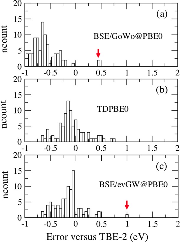
Histograms showing the number of transitions as a function of the difference in energy (eV) with respect to the theoretical TBE-2 best estimates data for (a) BSE/G₀W₀@PBE0, (b) TD-PBE0, and (c) BSE/GW@PBE0 results for all states in the Thiel set. The red arrows indicate the 2¹A_g states in hexatriene and octatetraene.

3.3. Additional Chromogens

In addition to the Thiel set, we decided to tackle a small set of molecules originating from dye chemistry. Our objective was to assess the performances of BSE/evGW@PBE0 for less “academic” structures. The treated compounds are displayed in Scheme 1. To obtain CC3 reference values, we have first selected quite compact molecules and, in particular, n → π* chromogens.¹¹² Indeed, our set includes members of the nitroso (1¹¹³ and 2(113)), thiorcarbonyl (3,¹¹⁴4¹¹⁵ and 5(116)), and diazo (6,¹¹⁷7,¹¹⁸ and 8(118)) families. We also added a bicyclic aromatic (9¹¹⁹), a well-known solvatochromic probe (10¹²⁰), two of the most popular fluorophores (11¹²¹ and 12(122)), and the photoactive trans-azobenzene (13¹²³) to represent medium-sized dyes. The results are listed in Tables 5 and 6.

Scheme 1. Representation of the Molecules under Investigation in Section 3.3.

Table 5. Computed Vertical Transition Energies (eV) for the First Ten Molecules Shown in Scheme 1^a.

		aug-cc-pVDZ				aug-cc-pVTZ				aug-cc-pVTZ		experimental
molecule	state	CC2	CCSD	CCSDR(3)	CC3	CC2	CCSD	CCSDR(3)	TBE	TD-PBE0	BSE/evGW@PBE0	ΔE	ref
1	A″ (n → π*)	1.985	1.983	1.970	1.980	1.958	1.958	1.943	1.953	1.772	1.513	1.82	(113)
2	A″(n → π*)	2.341	2.285	2.267	2.261	2.302	2.248	2.233	2.227	2.026	1.789	2.09	(113)
3	A2 (n → π*)	2.920	2.835	2.806	2.807	2.839	2.778	2.744	2.745	2.760	2.443	2.58	(114)
	A1 (π → π*)	5.348	5.348	5.209	5.172	5.263	5.285	5.140	5.103	5.025	4.724	4.81	(114)
4	A (n → π*)	2.344	2.296	2.249	2.248	2.295	2.257	2.208	2.207	2.121	1.895	2.14	(115)
	A (π→ π*)	6.704	6.747	6.550	6.491	6.598	6.617	6.425	6.366	6.010	5.518	b	(115)
5	A2 (n → π*)	4.010	3.864	3.814	3.802	3.934	3.814	3.764	3.752	3.741	3.432	3.52	(116)
	A1 (π→ π*)	6.551	6.455	6.332	6.298	6.455	6.382	6.257	6.223	6.271	5.823	6.08	(116)
6	Bg (n → π*)	3.765	3.775	3.735	3.743	3.692	3.702	3.665	3.673	3.477	3.283	3.65	(117)
7	A′ (n → π*)	3.935	3.949	3.900	3.903	3.882	3.898	3.856	3.859	3.655	3.473	3.64	(118)
8	B1 (n → π*)	3.514	3.540	3.492	3.494	3.466	3.494	3.494	3.496	3.477	3.283	3.29	(118)
9	B1 g (n → π*)	2.974	3.354	3.188	3.081	2.938	3.348	3.176	3.069	2.762	2.931	3.01	(119)
	B2u (π→ π*)	4.357	4.386	4.315	4.234	4.309	4.363	4.299	4.218	4.454	4.114	3.86	(119)
10	A1 (π→ π*)	3.952	4.285	4.106	3.964	3.925	4.278	4.106	3.964	3.905	3.800	3.59	(120)
MSE		0.132	0.161	0.077	0.045	0.072	0.112	0.033		–0.100	–0.345
MAE		0.147	0.161	0.078	0.045	0.100	0.112	0.036		0.143	0.345
RMSD		0.180	0.194	0.092	0.055	0.124	0.153	0.056		0.179	0.388
r		0.998	0.999	1.000	1.000	0.998	0.998	0.999		0.994	0.992

^aNote that the experimental values on the rightmost part of the table correspond to λ_max and cannot be compared directly to vertical theoretical estimates (see text). At the bottom of the table, the results of a statistical analysis using the TBE as a reference are given. MSE, MAE, and RMS are in eV; r is dimensionless.

^bA second band, as weak as the lowest n → π*, has been measured at ∼3.9 eV, but no π → π* was reported in the original work.

Table 6. Computed Vertical Transition Energies (eV) for the Last Three Molecules Shown in Scheme 1^a.

		aug-cc-pVDZ			aug-cc-pVTZ			aug-cc-pVTZ		experimental
molecule	state	CC2	CCSD	CCSDR(3)	CC2	CCSD	TBE	TD-PBE0	BSE/evGW@PBE0	ΔE	ref
11	A1 (π→ π*)	4.096	4.364	4.209	4.067	4.341	4.186	3.773	3.680	3.60	(121)
12	B2 (π→ π*)	2.923	2.888	2.821	2.906	2.896	2.829	3.134	2.725	2.46	(122)
13	Bg (n → π*)	2.884	3.006	2.940	2.836	2.968	2.902	2.621	2.540	2.76	(123)
	Bu (π→ π*)	4.069	4.380	4.228	4.036	4.350	4.198	3.704	3.696	3.92	(123)

^aSee Table 5 caption for more details.

For this set, we used MP2/aug-cc-pVTZ ground-state geometries and computed reference transition energies at the CC2, CCSD, CCSDR(3), and CC3 levels of theory using both aug-cc-pVDZ and aug-cc-pVTZ atomic basis sets. We followed a protocol very similar to the one of Thiel and co-workers¹⁷ to determine our own TBE. Indeed, for compounds 1–10 we determined TBE at the CC3 level,¹⁷ which was chosen as the best available single-reference method by first performing CC3/aug-cc-pVDZ calculations and next correcting for basis set effects using the difference between CCSDR(3)/aug-cc-pVDZ and CCSDR(3)/aug-cc-pVTZ transition energies. For five excited-states, it was possible to perform CC3/aug-cc-pVTZ computations, and the differences with respect to our reference TBE were smaller than 0.01 eV. For the three largest molecules (11–13, see Table 6), CC3 calculations are not technically possible, and the TBE estimates were obtained by correcting CCSDR(3)/aug-cc-pVDZ values for basis set effects determined at the CCSD level.

From Table 5, it appears that the basis sets effects for the EOM-CC calculations are relatively small: the use of the double-ζ basis set induces a mean increase of the computed transition energies by only ∼0.05 eV. Likewise, the use of noniterative triples [CCSDR(3)] provides a good approximation of the iterative triple results for the present set with an average deviation of 0.03 eV. It also appears that CC2 tends to give slightly more accurate estimates than CCSD, despite the larger computational cost of the latter. As expected, the various CC approaches provide extremely large correlation coefficients with respect to the TBE. All of these conclusions are well in line of the findings of previous works.^13,15,17 TD-PBE0 performs very well for the investigated series, providing a MSE of −0.10 eV (slight underestimation of the TBE) and a MAE of 0.14 eV in line of the one of CC2. TD-PBE0 also delivers an r of 0.99. These errors can be viewed as very small for TD-DFT^14,24 and this is in part related to the selection of n → π* chromogens for which TD-DFT is known to be especially accurate.^124,125 For the compounds of Table 5, BSE/evGW@PBE0 delivers less satisfying results than TD-DFT with an average error of 0.35 eV and a systematic underestimation of the reference values (see Figure 9a). These underestimations are especially strong for the most compact molecules for which deviations exceeding 0.40 eV can be found. In fact, BSE/evGW@PBE0 outperforms TD-PBE0 for only the two states of compound 9 (the largest compound of Table 5) for which it provides a splitting between the two states of 1.18 eV, which is in much better agreement with the TBE value (1.15 eV) than TD-PBE0 (1.69 eV). Given the fact that BSE/evGW@PBE0 transition energies were also too small for the most compact structures of Thiel’s set, namely ethene and formaldehyde, for which BSE/evGW@PBE0 underestimates the lowest lying TBE-2 excitations by 0.48 and 0.47 eV, respectively, we suspected that the smallest possible chromogens (constituted of two atoms and three “active” orbitals: n, π, and π*) are particularly challenging for BSE. For this reason, we also considered the largest systems listed in Table 6. Although this set is too small to draw statistical conclusions, we note that, for 11 and 13, both TD-PBE0 and BSE/evGW@PBE0 are significantly smaller than the reference values but the deviations between the two approaches remain below 0.1 eV. For 12, BSE provides a value significantly smaller than that of TD-PBE0 but in much better agreement with the TBE. In short, it indeed appears that BSE/evGW@PBE0 has difficulties in describing very compact structures. In Figure 9a, one indeed notices that the blue squares corresponding to the smallest systems deviate more significantly from the TBE than the red circles corresponding to medium-sized chromogens. We tentatively ascribe this outcome to the so-called self-screening problem in the limit of very few electrons.¹²⁶ While such a statement clearly calls for more fundamental investigations, we believe that these problems become of much less relevance for medium to large size molecules for which BSE is more useful.

Figure 9.

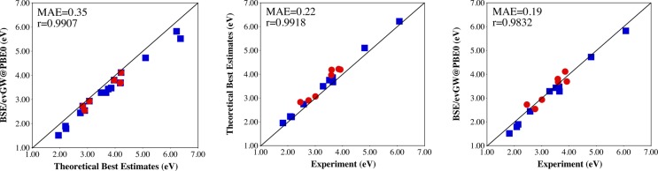
Comparisons between: BSE and TBE values (left); experimental and TBE values (center); experimental and BSE values (right) for the set of transitions listed in Tables 5 and 6. The blue squares (red dots) correspond to the first eight (last five) dyes of Scheme 1.

Let us now turn to comparisons with the available experimental values shown in Figure 9b and c. We underline that these values correspond to experimental λ_max and cannot therefore be rigorously compared to theoretical vertical transition energies. This is why the TBE values are systematically larger than their experimental counterparts that are influenced by geometrical and vibrational relaxation effects. This deviation attains 0.22 eV on average, which is consistent with previously reported amplitudes for these relaxation effects.^127−131 Nevertheless, the TBE and experimental values correlate very well (r = 0.991). When comparing the BSE/evGW@PBE0 energies to experimental values, one obtains a match that is superior to the one reported at the bottom of Table 5. Indeed, as shown in Figure 9c, the correlation is excellent (r = 0.983) and the mean absolute deviation attains only 0.19 eV. This result obviously originates from an error compensation mechanism and illustrates that special care must be taken when comparing vertical theoretical excitation energies to experimental λ_max. This also strongly suggests that calculations of 0–0 energies with BSE would be welcome⁶⁴ with the delicate issue of calculating (analytic) forces in the excited states within the BSE formalism.¹³²

4. Conclusions and Outlook

We have assessed the accuracy of the Bethe–Salpeter formalism in its standard adiabatic implementation for the calculation of the vertical excitation energies of small- and medium-sized organic molecules. To this end, we have applied a large diffuse-containing atomic basis set, namely aug-cc-pVTZ, and considered the set of 28 compounds proposed by Thiel and co-workers, together with a new set of small dye chromophores constituted of 13 molecules and 18 transitions to low-lying excited-states for which theoretical best estimates have been obtained.

Several conclusions can be drawn from the present study. The first important finding is that the “standard” Bethe–Salpeter calculations based on non-self-consistent G₀W₀ calculations starting from Kohn–Sham eigenstates generated with semilocal functionals, such as PBE, dramatically underestimate transition energies. The situation improves when starting with a global hybrid such as PBE0 even though the resulting excitation energies are still too small with a mean absolute error of ∼0.6 eV.

Although adjusting the starting functional may be an interesting solution, we have shown that a simple self-consistent-scheme with updates of the quasiparticle energies allows for the BSE excitation energies to be brought into much better agreement with the theoretical best estimate, with an MAE of ∼0.25 eV, and a small dependency on the starting functional related to the Kohn–Sham wave functions that are kept frozen. Indeed, the BSE/evGW@PBE and BSE/evGW@PBE0 agree within 80 meV (MAE) with a linear regression coefficient of 0.998. With such a self-consistent scheme, the BSE approach yields a mean average error within 20 meV of the most accurate TD-DFT calculations obtained with the PBE0 XC functional.

The present findings concerning the stability with respect to the starting functional are consistent with early observations in sp-bonded solids⁴⁰ that the Kohn–Sham wave functions, even calculated with local functionals, agree nicely with the quasiparticle ones, even though the Kohn–Sham and GW energy differ significantly. This conclusion should be mitigated in the case of tight 3d orbitals, for example, where due to significant self-interaction the Kohn–Sham wave functions may differ significantly from ones of the self-consistent GW.^76,88−90 In the case of molecular systems, a recent GW/BSE study of cyanines⁶³ demonstrated that Kohn–Sham and self-consistent GW wave functions (within the static COHSEX approximation) would hardly differ for occupied levels. Deviations could be observed for unoccupied states but with an impact on the BSE absorption energy no larger than 0.2 eV. Special care must be taken with such small molecules, however, because the LUMO level is bound within DFT-PBE, for example, but unbound (negative electronic affinity) within GW, a situation that does not occur for larger molecules.

The overall comparison should be mitigated by a closer inspection of specific cases. As a first observation, it seems that the Bethe–Salpeter formalism faces difficulties for tiny molecules, yielding transition energies located 0.4–0.5 eV too low in energy relative to reference data, even in the present self-consistent implementation. Further investigation on a larger set of very small molecules should be conducted. Such a tendency, which may be attributed to the self-screening problem,⁹⁷ is probably of limited practical importance because it disappears for small molecules such as benzene and the nucleobases.

A second potentially important difference between TD-PBE0 and BSE was found during the analysis of the transitions displaying significant multiple-excitation character. For such transitions, differences as large as 0.5 eV can be observed between TDP-BE0 and BSE. Although not affecting the overall statistics much (they represent only ∼10% of the transitions considered here), they bear significant conceptual importance because the present Bethe–Salpeter implementation is adiabatic. Although the BSE formalism tends to worsen the comparison with the theoretical best estimate (TBE-2), as compared to TD-PBE0, for the 2¹A_g transition in both octatetraene and hexatriene, it is found to dramatically improve the agreement with TBE-2 in the case of transitions in aromatic molecules with a large multiple-excitation weight. In all cases, the BSE formalism comes much closer to CC2 or CCSDR(3) data than TD-PBE0 for such transitions, and even yields more accurate results than CC2. Such a different behavior between TD-PBE0 and BSE, both adiabatic in their present implementation, is a remarkable finding that needs further investigation.

In a recent study by Rebolini and co-workers on the excitations of the paradigmatic H₂ molecule as a function of bond length,¹³³ it was noted that model Bethe–Salpeter calculations starting from an independent-particle polarizability based on the “exact” one-particle Green’s function (that is, a Green’s function with poles at the proper quasiparticle energies, including further satellites) could very nicely reproduce the second singlet excitation energy bearing significant double-excitation character. Such an observation is very consistent with what we observe during our study of transitions with multiple excitation character starting from self-consistent GW calculations providing correct quasiparticle energies to build the needed polarizability. The authors concluded, as we do, that it is indeed remarkable that such an adiabatic formalism may apparently capture some multiple-excitation character.

As another recent example, it was demonstrated in the case of the cyanine family^63,64 that the same adiabatic self-consistent Bethe–Salpeter approach provides the lowest singlet excitation energies in very close agreement with exCC3 reference calculations, whereas standard TD-DFT calculations with various semilocal, global, or range-separated hybrid functionals deliver excitation energies that are significantly too large. This is again very consistent with what was observed here in the case of the aromatic molecule transitions showing significant multiexcitation character (see Table 2).

Although such evidence seems to validate the idea that the Bethe–Salpeter formalism, even in its adiabatic formulation, yields superior results to those of TD-DFT for such problematic transitions, further tests should be performed on a larger set of transitions displaying multiexcitation character. Further, it would be interesting to conduct Bethe–Salpeter calculations with dynamical screening. Inclusion of dynamical screening is expected to lower the excitation energies of such transitions,⁹⁶ which may not play in favor of improving the agreement with reference TBE-2 calculations (see Table 2).

Overall, the good agreement with the best TD-DFT calculations for the present set of molecules, the ability to tackle charge-transfer excitations, the lack of dependency with respect to the starting functional in the present case of self-consistent GW calculations, and, potentially, more favorable behavior than TD-DFT for transitions with multiple-excitation character are encouraging results for the use of the present adiabatic implementation of the Bethe–Salpeter formalism. Although Bethe–Salpeter calculations require the same computational effort as TD-DFT calculations, the preceding GW calculations, even though offering an O(N⁴) scaling in the present Coulomb-fitting implementation, still remain more demanding than standard DFT calculations. On that account, the recent efforts to provide accurate quasiparticle energies within generalized Kohn–Sham formalisms stand as a very competitive approach to serve as a starting point for Bethe–Salpeter calculations. It would be interesting to explore the merits of TD-DFT calculations based on such functionals with respect to transitions with multiple-excitation character.

Supporting Information Available

Convergence tests, tables with all values of transition energies, and Cartesian coordinates for compounds 1–13. The Supporting Information is available free of charge on the ACS Publications website at DOI: 10.1021/acs.jctc.5b00304.

The authors declare no competing financial interest.

References

- Runge E.; Gross E. K. U. Phys. Rev. Lett. 1984, 52, 997–1000. [Google Scholar]
- Casida M. E.Recent Advances in Density Functional Methods. In Time-Dependent Density-Functional Response Theory for Molecules; Chong D. P., Ed.; World Scientific: Singapore, 1995; Vol. 1, pp 155–192. [Google Scholar]
- Schirmer J.; Trofimov A. B. J. Chem. Phys. 2004, 120, 11449–11464. [DOI] [PubMed] [Google Scholar]
- Hellweg A.; Grün S. A.; Hättig C. Phys. Chem. Chem. Phys. 2008, 10, 4119–4127. [DOI] [PubMed] [Google Scholar]
- Krauter C. M.; Pernpointner M.; Dreuw A. J. Chem. Phys. 2013, 138, 044107. [DOI] [PubMed] [Google Scholar]
- Stanton J. F.; Bartlett R. J. J. Chem. Phys. 1993, 98, 7029–7039. [Google Scholar]
- Kállay M.; Gauss J. J. Chem. Phys. 2004, 121, 9257–9269. [DOI] [PubMed] [Google Scholar]
- Caricato M. J. Chem. Phys. 2013, 139, 114103. [DOI] [PubMed] [Google Scholar]
- Nakatsuji H. J. Chem. Phys. 1991, 94, 6716–6727. [Google Scholar]
- Nakatsuji H.; Ehara M. J. Chem. Phys. 1993, 98, 7179–7184. [Google Scholar]
- Andersson K.; Malmqvist P.; Roos B. O. J. Chem. Phys. 1992, 96, 1218–1226. [Google Scholar]
- Buenker R. J.; Peyerimhoff S. D. Theor. Chim. Acta 1968, 12, 183–199. [Google Scholar]
- Schreiber M.; Silva-Junior M. R.; Sauer S. P. A.; Thiel W. J. Chem. Phys. 2008, 128, 134110. [DOI] [PubMed] [Google Scholar]
- Silva-Junior M. R.; Schreiber M.; Sauer S. P. A.; Thiel W. J. Chem. Phys. 2008, 129, 104103. [DOI] [PubMed] [Google Scholar]
- Sauer S. P. A.; Schreiber M.; Silva-Junior M. R.; Thiel W. J. Chem. Theory Comput. 2009, 5, 555–564. [DOI] [PubMed] [Google Scholar]
- Silva-Junior M. R.; Thiel W. J. Chem. Theory Comput. 2010, 6, 1546–1564. [DOI] [PubMed] [Google Scholar]
- Silva-Junior M. R.; Sauer S. P. A.; Schreiber M.; Thiel W. Mol. Phys. 2010, 108, 453–465. [Google Scholar]
- Silva-Junior M. R.; Schreiber M.; Sauer S. P. A.; Thiel W. J. Chem. Phys. 2010, 133, 174318. [DOI] [PubMed] [Google Scholar]
- Trani F.; Scalmani G.; Zheng G. S.; Carnimeo I.; Frisch M. J.; Barone V. J. Chem. Theory Comput. 2011, 7, 3304–3313. [DOI] [PubMed] [Google Scholar]
- Voityuk A. A. J. Chem. Theory Comput. 2014, 10, 4950–4958. [DOI] [PubMed] [Google Scholar]
- Harbach P. H. P.; Wormit M.; Dreuw A. J. Chem. Phys. 2014, 141, 064113. [DOI] [PubMed] [Google Scholar]
- Kánnár D.; Szalay P. G. J. Chem. Theory Comput. 2014, 10, 3757–3765. [DOI] [PubMed] [Google Scholar]
- Goerigk L.; Moellmann J.; Grimme S. Phys. Chem. Chem. Phys. 2009, 11, 4611–4620. [DOI] [PubMed] [Google Scholar]
- Jacquemin D.; Wathelet V.; Perpète E. A.; Adamo C. J. Chem. Theory Comput. 2009, 5, 2420–2435. [DOI] [PubMed] [Google Scholar]
- Rohrdanz M. A.; Martins K. M.; Herbert J. M. J. Chem. Phys. 2009, 130, 054112. [DOI] [PubMed] [Google Scholar]
- Jacquemin D.; Perpète E. A.; Ciofini I.; Adamo C. J. Chem. Theory Comput. 2010, 6, 1532–1537. [DOI] [PubMed] [Google Scholar]
- Jacquemin D.; Perpète E. A.; Ciofini I.; Adamo C.; Valero R.; Zhao Y.; Truhlar D. G. J. Chem. Theory Comput. 2010, 6, 2071–2085. [DOI] [PubMed] [Google Scholar]
- Mardirossian N.; Parkhill J. A.; Head-Gordon M. Phys. Chem. Chem. Phys. 2011, 13, 19325–19337. [DOI] [PubMed] [Google Scholar]
- Jacquemin D.; Perpète E. A.; Ciofini I.; Adamo C. Theor. Chem. Acc. 2011, 128, 127–136. [Google Scholar]
- Jacquemin D.; Mennucci B.; Adamo C. Phys. Chem. Chem. Phys. 2011, 13, 16987–16998. [DOI] [PubMed] [Google Scholar]
- Huix-Rotllant M.; Ipatov A.; Rubio A.; Casida M. E. Chem. Phys. 2011, 391, 120–129. [Google Scholar]
- Della Sala F.; Fabiano E. Chem. Phys. 2011, 391, 19–26. [Google Scholar]
- Jacquemin D.; Zhao Y.; Valero R.; Adamo C.; Ciofini I.; Truhlar D. G. J. Chem. Theory Comput. 2012, 8, 1255–1259. [DOI] [PubMed] [Google Scholar]
- Peverati R.; Truhlar D. G. Phys. Chem. Chem. Phys. 2012, 14, 11363–11370. [DOI] [PubMed] [Google Scholar]
- Ziegler T.; Krykunov M.; Cullen J. J. Chem. Phys. 2012, 136, 124107. [DOI] [PMC free article] [PubMed] [Google Scholar]
- Hedin L. Phys. Rev. A 1965, 139, 796–823. [Google Scholar]
- Sham L. J.; Rice T. M. Phys. Rev. 1966, 144, 708–714. [Google Scholar]
- Hanke W.; Sham L. J. Phys. Rev. Lett. 1979, 43, 387–390. [Google Scholar]
- Strinati G. Phys. Rev. Lett. 1982, 49, 1519–1522. [Google Scholar]
- Hybertsen M. S.; Louie S. G. Phys. Rev. B 1986, 34, 5390–5413. [DOI] [PubMed] [Google Scholar]
- Godby R. W.; Schlüter M.; Sham L. J. Phys. Rev. B 1988, 37, 10159–10175. [DOI] [PubMed] [Google Scholar]
- Salpeter E. E.; Bethe H. A. Phys. Rev. 1951, 84, 1232–1242. [Google Scholar]
- Rohlfing M.; Louie S. G. Phys. Rev. Lett. 1998, 80, 3320–3323. [Google Scholar]
- Benedict L. X.; Shirley E. L.; Bohn R. B. Phys. Rev. Lett. 1998, 80, 4514–4517. [Google Scholar]
- Albrecht S.; Reining L.; Del Sole R.; Onida G. Phys. Rev. Lett. 1998, 80, 4510–4513. [Google Scholar]
- Tiago M. L.; Chelikowsky J. R. Solid State Commun. 2005, 136, 333–337. [Google Scholar]
- Tiago M. L.; Kent P. R. C.; Hood R. Q.; Reboredo F. A. J. Chem. Phys. 2008, 129, 084311. [DOI] [PubMed] [Google Scholar]
- Foerster D.; Koval P.; Sanchez-Portal D. J. Chem. Phys. 2011, 135, 074105. [DOI] [PubMed] [Google Scholar]
- Palummo M.; Hogan C.; Sottile F.; Bagalá P.; Rubio A. J. Chem. Phys. 2009, 131, 084102. [DOI] [PubMed] [Google Scholar]
- Kaczmarski M. S.; Ma Y.; Rohlfing M. Phys. Rev. B 2010, 81, 115433. [Google Scholar]
- Ma Y.; Rohlfing M.; Molteni C. J. Chem. Theory Comput. 2010, 6, 257–265. [DOI] [PubMed] [Google Scholar]
- Rocca D.; Lu D.; Galli G. J. Chem. Phys. 2010, 133, 164109. [DOI] [PubMed] [Google Scholar]
- Garcia-Lastra J. M.; Thygesen K. S. Phys. Rev. Lett. 2011, 106, 187402. [DOI] [PubMed] [Google Scholar]
- Blase X.; Attaccalite C. Appl. Phys. Lett. 2011, 99, 171909. [Google Scholar]
- Duchemin I.; Deutsch T.; Blase X. Phys. Rev. Lett. 2012, 109, 167801. [DOI] [PubMed] [Google Scholar]
- Baumeier B.; Andrienko D.; Ma Y.; Rohlfing M. J. Chem. Theory Comput. 2012, 8, 997–1002. [DOI] [PubMed] [Google Scholar]
- Faber C.; Duchemin I.; Deutsch T.; Blase X. Phys. Rev. B 2012, 86, 155315. [DOI] [PubMed] [Google Scholar]
- Hogan C.; Palummo M.; Gierschner J.; Rubio A. J. Chem. Phys. 2013, 138, 024312. [DOI] [PubMed] [Google Scholar]
- Faber C.; Boulanger P.; Duchemin I.; Attaccalite C.; Blase X. J. Chem. Phys. 2013, 139, 194308. [DOI] [PubMed] [Google Scholar]
- Varsano D.; Coccia E.; Pulci O.; Mosca Conte A.; Guidoni L. Comput. Theor. Chem. 2014, 1040–1041, 338–346. [Google Scholar]
- Coccia E.; Varsano D.; Guidoni L. J. Chem. Theory Comput. 2014, 10, 501–506. [DOI] [PMC free article] [PubMed] [Google Scholar]
- Baumeier B.; Rohlfing M.; Andrienko D. J. Chem. Theory Comput. 2014, 10, 3104–3110. [DOI] [PubMed] [Google Scholar]
- Boulanger P.; Jacquemin D.; Duchemin I.; Blase X. J. Chem. Theory Comput. 2014, 10, 1212–1218. [DOI] [PubMed] [Google Scholar]
- Boulanger P.; Chibani S.; Le Guennic B.; Duchemin I.; Blase X.; Jacquemin D. J. Chem. Theory Comput. 2014, 10, 4548–4556. [DOI] [PubMed] [Google Scholar]
- Koval P.; Foerster D.; Sánchez-Portal D. Phys. Rev. B 2014, 89, 155417. [Google Scholar]
- Hahn T.; Geiger J.; Blase X.; Duchemin I.; Niedzialek D.; Tscheuschner S.; Beljonne D.; Bässler H.; Köhler A. Adv. Funct. Mater. 2015, 25, 1287–1295. [Google Scholar]
- Krause K.; Harding M. E.; Klopper W. Mol. Phys. 2015, 10.1080/00268976.2015.1025113. [DOI] [Google Scholar]
- Tozer D. J. J. Chem. Phys. 2003, 119, 12697–12699. [Google Scholar]
- Dreuw A.; Head-Gordon M. J. Am. Chem. Soc. 2004, 126, 4007–4016. [DOI] [PubMed] [Google Scholar]
- Le Guennic B.; Jacquemin D. Acc. Chem. Res. 2015, 48, 530–537. [DOI] [PMC free article] [PubMed] [Google Scholar]
- Martin P. C.; Schwinger J. Phys. Rev. 1959, 115, 1342–1373. [Google Scholar]
- Perdew J. P.; Burke K.; Ernzerhof M. Phys. Rev. Lett. 1996, 77, 3865–3868. [DOI] [PubMed] [Google Scholar]
- Adamo C.; Barone V. J. Chem. Phys. 1999, 110, 6158–6170. [Google Scholar]
- Ernzerhof M.; Scuseria G. E. J. Chem. Phys. 1999, 110, 5029–5036. [Google Scholar]
- Hahn P. H.; Schmidt W. G.; Bechstedt F. Phys. Rev. B 2005, 72, 245425. [Google Scholar]
- Rostgaard C.; Jacobsen K. W.; Thygesen K. S. Phys. Rev. B 2010, 81, 085103. [Google Scholar]
- Blase X.; Attaccalite C.; Olevano V. Phys. Rev. B 2011, 83, 115103. [Google Scholar]
- Faber C.; Attaccalite C.; Olevano V.; Runge E.; Blase X. Phys. Rev. B 2011, 83, 115123. [Google Scholar]
- Marom N.; Moussa J. E.; Ren X.; Tkatchenko A.; Chelikowsky J. R. Phys. Rev. B 2011, 84, 245115. [Google Scholar]
- Marom N.; Caruso F.; Ren X.; Hofmann O. T.; Körzdörfer T.; Chelikowsky J. R.; Rubio A.; Scheffler M.; Rinke P. Phys. Rev. B 2012, 86, 245127. [Google Scholar]
- Körzdörfer T.; Marom N. Phys. Rev. B 2012, 86, 041110. [Google Scholar]
- Bruneval F.; Marques M. A. L. J. Chem. Theory Comput. 2013, 9, 324–329. [DOI] [PubMed] [Google Scholar]
- Pham T. A.; Nguyen H.-V.; Rocca D.; Galli G. Phys. Rev. B 2013, 87, 155148. [Google Scholar]
- Caruso F.; Rinke P.; Ren X.; Rubio A.; Scheffler M. Phys. Rev. B 2013, 88, 075105. [DOI] [PubMed] [Google Scholar]
- Lischner J.; Sharifzadeh S.; Deslippe J.; Neaton J. B.; Louie S. G. Phys. Rev. B 2014, 90, 115130. [Google Scholar]
- Kümmel S.; Kronik L. Rev. Mod. Phys. 2008, 80, 3–60. [Google Scholar]
- Borghi G.; Ferretti A.; Nguyen N. L.; Dabo I.; Marzari N. Phys. Rev. B 2014, 90, 075135. [DOI] [PubMed] [Google Scholar]
- Bruneval F.; Vast N.; Reining L. Phys. Rev. B 2006, 74, 045102. [DOI] [PubMed] [Google Scholar]
- Gatti M.; Bruneval F.; Olevano V.; Reining L. Phys. Rev. Lett. 2007, 99, 266402. [DOI] [PubMed] [Google Scholar]
- Trani F.; Vidal J.; Botti S.; Marques M. A. L. Phys. Rev. B 2010, 82, 085115. [DOI] [PubMed] [Google Scholar]
- Rangel T.; Kecik D.; Trevisanutto P. E.; Rignanese G.-M.; Van Swygenhoven H.; Olevano V. Phys. Rev. B 2012, 86, 125125. [Google Scholar]
- Körbel S.; Boulanger P.; Duchemin I.; Blase X.; Marques M. A. L.; Botti S. J. Chem. Theory Comput. 2014, 10, 3934–3943. [DOI] [PubMed] [Google Scholar]
- Refaely-Abramson S.; Sharifzadeh S.; Govind N.; Autschbach J.; Neaton J. B.; Baer R.; Kronik L. Phys. Rev. Lett. 2012, 109, 226405. [DOI] [PubMed] [Google Scholar]
- Elliott P.; Goldson S.; Canahui C.; Maitra N. T. Chem. Phys. 2011, 391, 110–119. [Google Scholar]
- Ullrich C.Time-Dependent Density-Functional Theory: Concepts and Applications, Oxford Graduate Texts; Oxford University Press: New York, 2012. [Google Scholar]
- Ma Y.; Rohlfing M.; Molteni C. Phys. Rev. B 2009, 80, 241405. [Google Scholar]
- Romaniello P.; Sangalli D.; Berger J. A.; Sottile F.; Molinari L. G.; Reining L.; Onida G. J. Chem. Phys. 2009, 130, 044108. [DOI] [PubMed] [Google Scholar]
- Dunning T. H. J. Chem. Phys. 1989, 90, 1007–1023. [Google Scholar]
- Kendall R. A.; Dunning T. H.; Harisson R. J. J. Chem. Phys. 1992, 96, 6796–6806. [Google Scholar]
- Valiev M.; Bylaska E. J.; Govind N.; Kowalski K.; Straatsma T. P.; Van Dam H. J. J.; Wang D.; Nieplocha J.; Apra E.; Windus T. L.; de Jong W. A. Comput. Phys. Commun. 2010, 181, 1477–1489. [Google Scholar]
- Weigend F.; Köhn A.; Hättig C. J. Chem. Phys. 2002, 116, 3175–3183. [Google Scholar]
- Frisch M. J.; Trucks G. W.; Schlegel H. B.; Scuseria G. E.; Robb M. A.; Cheeseman J. R.; Scalmani G.; Barone V.; Mennucci B.; Petersson G. A.; Nakatsuji H.; Caricato M.; Li X.; Hratchian H. P.; Izmaylov A. F.; Bloino J.; Zheng G.; Sonnenberg J. L.; Hada M.; Ehara M.; Toyota K.; Fukuda R.; Hasegawa J.; Ishida M.; Nakajima T.; Honda Y.; Kitao O.; Nakai H.; Vreven T.; Montgomery J. A. Jr.; Peralta J. E.; Ogliaro F.; Bearpark M.; Heyd J. J.; Brothers E.; Kudin K. N.; Staroverov V. N.; Kobayashi R.; Normand J.; Raghavachari K.; Rendell A.; Burant J. C.; Iyengar S. S.; Tomasi J.; Cossi M.; Rega N.; Millam J. M.; Klene M.; Knox J. E.; Cross J. B.; Bakken V.; Adamo C.; Jaramillo J.; Gomperts R.; Stratmann R. E.; Yazyev O.; Austin A. J.; Cammi R.; Pomelli C.; Ochterski J. W.; Martin R. L.; Morokuma K.; Zakrzewski V. G.; Voth G. A.; Salvador P.; Dannenberg J. J.; Dapprich S.; Daniels A. D.; Farkas O.; Foresman J. B.; Ortiz J. V.; Cioslowski J.; Fox D. J.. Gaussian 09, revision D.01; Gaussian Inc.: Wallingford, CT, 2009. [Google Scholar]
- TURBOMOLE, V6.6; a development of University of Karlsruhe and Forschungszentrum Karlsruhe GmbH, 1989–2007, TURBOMOLE GmbH, since 2007. (2014); available from http://www.turbomole.com. [Google Scholar]
- Aidas K.; Angeli C.; Bak K. L.; Bakken V.; Bast R.; Boman L.; Christiansen O.; Cimiraglia R.; Coriani S.; Dahle P.; Dalskov E. K.; Ekström U.; Enevoldsen T.; Eriksen J. J.; Ettenhuber P.; Fernández B.; Ferrighi L.; Fliegl H.; Frediani L.; Hald K.; Halkier A.; Hättig C.; Heiberg H.; Helgaker T.; Hennum A. C.; Hettema H.; Hjertenæs E.; Høst S.; Høyvik I.-M.; Iozzi M. F.; Jansík B.; Jensen H. J. A.; Jonsson D.; Jørgensen P.; Kauczor J.; Kirpekar S.; Kjærgaard T.; Klopper W.; Knecht S.; Kobayashi R.; Koch H.; Kongsted J.; Krapp A.; Kristensen K.; Ligabue A.; Lutnæs O. B.; Melo J. I.; Mikkelsen K. V.; Myhre R. H.; Neiss C.; Nielsen C. B.; Norman P.; Olsen J.; Olsen J. M. H.; Osted A.; Packer M. J.; Pawlowski F.; Pedersen T. B.; Provasi P. F.; Reine S.; Rinkevicius Z.; Ruden T. A.; Ruud K.; Rybkin V. V.; Sałek P.; Samson C. C. M.; de Merás A. S.; Saue T.; Sauer S. P. A.; Schimmelpfennig B.; Sneskov K.; Steindal A. H.; Sylvester-Hvid K. O.; Taylor P. R.; Teale A. M.; Tellgren E. I.; Tew D. P.; Thorvaldsen A. J.; Thøgersen L.; Vahtras O.; Watson M. A.; Wilson D. J. D.; Ziolkowski M.; Ågren H. Wiley Interdiscip. Rev.: Comput. Mol. Sci. 2014, 4, 269–284. [DOI] [PMC free article] [PubMed] [Google Scholar]
- Roca-Sanjuán D.; Rubio M.; Merchán M.; Serrano-Andrés L. J. Chem. Phys. 2006, 125, 084302. [DOI] [PubMed] [Google Scholar]
- Qian X.; Umari P.; Marzari N. Phys. Rev. B 2011, 84, 075103. [Google Scholar]
- von Barth U.; Holm B. Phys. Rev. B 1996, 54, 8411–8419. [DOI] [PubMed] [Google Scholar]
- Shishkin M.; Kresse G. Phys. Rev. B 2007, 75, 235102. [DOI] [PubMed] [Google Scholar]
- Marques M. A. L., Nogueira F. M. S., Gross E. K. U., Rubio A., Eds. Fundamentals of Time-Dependent Density Functional Theory, Lecture Notes in Physics; Springer-Verlag: Heidelberg, 2012; Vol. 837, p 592. [Google Scholar]
- Note that here the wording “multiple-excitations character” refers to excitations that cannot be obtained accurately by a linear combination of determinants obtained by promoting a single-electron from the ground-state Hartree–Fock–Slater determinant. This follows the coupled-cluster “single excitation” T1 percentage that gives the weight of such determinants in the excited-state many-body wave functions. A value under 90% is generally considered as indicating a significant contribution from multiple excitations.
- Comparison with a wavelet-based code (BigDFT134,135) indicates that, at the DFT level, such a state wants to delocalize much more than allowed by the aug-cc-pVTZ basis.
- Griffiths J.Colour and Constitution of Organic Molecules; Academic Press: London, 1976; pp 1–290. [Google Scholar]
- Tarte P. Bull. Soc. Chim. Belg. 1954, 63, 525–541. [Google Scholar]
- Barrett J.; Deghaidy F. S. Spectrochim. Acta, Part A 1975, 31, 707–713. [Google Scholar]
- Middleton W. J.; Howard E. G.; Sharkey W. H. J. Org. Chem. 1965, 30, 1375–1384. [Google Scholar]
- Downs A. J. J. Chem. Soc. 1962, 4361–4366. [Google Scholar]
- Collier S. S.; Slater D. H.; Calvert J. G. Photochem. Photobiol. 1968, 7, 737–753. [Google Scholar]
- Mirbach M. J.; Liu K. C.; Mirbach M. F.; Cherry W. R.; Turro N. J.; Engel P. S. J. Am. Chem. Soc. 1978, 100, 5122–5129. [Google Scholar]
- Hurst J. K.; Wormell P.; Krausz E.; Lacey A. R. Chem. Phys. 1999, 246, 229–246. [Google Scholar]
- Lagalante A. F.; Jacobson R. J.; Bruno T. J. J. Org. Chem. 1996, 61, 6404–6406. [DOI] [PubMed] [Google Scholar]
- Wintgens V.; Valat P.; Kossanyi J.; Biczok L.; Demeter A.; Berces T. J. Chem. Soc. Faraday Trans. 1994, 90, 411–421. [Google Scholar]
- Arroyo I. J.; Hu R.; Merino G.; Tang B. Z.; Pena-Cabrera E. J. Org. Chem. 2009, 74, 5719–5722. [DOI] [PubMed] [Google Scholar]
- Perkampus H. H.UV/Vis. Atlas of Organic Compounds, 2nd ed.; VCH: Weinheim, 19921–336 and 1–1525. [Google Scholar]
- Jacquemin D.; Perpète E. A.; Scalmani G.; Frisch M. J.; Kobayashi R.; Adamo C. J. Chem. Phys. 2007, 126, 144105. [DOI] [PubMed] [Google Scholar]
- Jacquemin D.; Perpète E. A.; Ciofini I.; Adamo C. Theor. Chem. Acc. 2008, 120, 405–410. [Google Scholar]
- Romaniello P.; Guyot S.; Reining L. J. Chem. Phys. 2009, 131, 154111. [DOI] [PubMed] [Google Scholar]
- Goerigk L.; Grimme S. J. Chem. Phys. 2010, 132, 184103. [Google Scholar]
- Send R.; Kühn M.; Furche F. J. Chem. Theory Comput. 2011, 7, 2376–2386. [DOI] [PubMed] [Google Scholar]
- Jacquemin D.; Planchat A.; Adamo C.; Mennucci B. J. Chem. Theory Comput. 2012, 8, 2359–2372. [DOI] [PubMed] [Google Scholar]
- Winter N. O. C.; Graf N. K.; Leutwyler S.; Hattig C. Phys. Chem. Chem. Phys. 2013, 15, 6623–6630. [DOI] [PubMed] [Google Scholar]
- Fang X.; Wang Y.; Wang D.; Zhao G.; Zhang W.; Ren A.; Wang H.; Xu J.; Gao B.-R.; Yang W. J. Phys. Chem. Lett. 2014, 5, 92–98. [DOI] [PubMed] [Google Scholar]
- Ismail-Beigi S.; Louie S. G. Phys. Rev. Lett. 2003, 90, 076401. [DOI] [PubMed] [Google Scholar]
- Rebolini E.; Toulouse J.; Savin A. In Concepts and Methods in Modern Theoretical Chemistry: Electronic Structure and Reactivity; Ghosh S. K., Chattaraj P. K., Eds.; CRC Press, 2013; pp 367–390. [Google Scholar]
- Genovese L.; Neelov A.; Goedecker S.; Deutsch T.; Ghasemi S. A.; Willand A.; Caliste D.; Zilberberg O.; Rayson M.; Bergman A.; Schneider R. J. Chem. Phys. 2008, 129, 014109. [DOI] [PubMed] [Google Scholar]
- Mohr S.; Ratcliff L. E.; Boulanger P.; Genovese L.; Caliste D.; Deutsch T.; Goedecker S. J. Chem. Phys. 2014, 140, 204110. [DOI] [PubMed] [Google Scholar]
Associated Data
This section collects any data citations, data availability statements, or supplementary materials included in this article.