A new approach for optical assessment of directional anisotropy in turbid media

Abstract

A study of polarized light transport in scattering media exhibiting directional anisotropy or linear birefringence is presented in this paper. Novel theoretical and experimental methodologies for the quantification of birefringent alignment based on out-of-plane polarized light transport are presented here. A polarized Monte Carlo model and a polarimetric imaging system were devised to predict and measure the impact of birefringence on an impinging linearly polarized light beam. Ex-vivo experiments conducted on bovine tendon, a biological sample consisting of highly packed type I collagen fibers with birefringent property, showed good agreement with the analytical results.

Top view geometry of the in-plane (a) and the out-of-plane (b) detection. Letter C indicates the location of the detection arm.

1. Introduction

Polarization filtering and gating have been used in several biomedical applications. Polarized microscopy is commonly used in characterizing biological media, that is generally highly scattering and depolarizing [1], but other techniques have also surfaced in the last few years and have been used to investigate structural, mechanical, and scattering properties of biological bulk tissue [2–9]. Kunnen et al. have recently demonstrated the use of optical polarimetry to characterize cancerous and non-cancerous tissue samples [9]. They studied the interaction of elliptically polarized light with Intralipid tissue-like phantoms and lung tissue by analyzing the Stokes vector of the back-scattered light.

When observing collagenous and birefringent media, polarization sensitive optical coherence tomography (PS-OCT) has shown some interesting results [10–16]. De Boer et al. [10] and Yang et al. [11] utilized PS-OCT for a tendon structural study. The former group provided 2D depth-resolved birefringence images of bovine tendon to investigate the effect of thermal injuries and pathological changes of birefringence material during laser therapy. The latter group applied the same imaging technique to chicken tendon to find the relationship between birefringence and optical properties. Pierce et al. [12] used PS-OCT for human burn injury diagnosis, while Oh et al. [13] used the same technique for wound healing analysis on a rabbit wound model, in which they tried to visualize collagen regeneration. Jiao et al. [14] reconstructed 2D depth-resolved Mueller matrices of biological tissue and showed that this technique could be used to measure optical polarization properties of a sample. Götzinger et al. [15] utilized a similar imaging system to provide high quality 3D images from healthy and diseased human retinas for diagnostic purposes. Duan et al. [16] used PS-OCT images to identify basal cell carcinoma of mouse skin. They developed a classifier to analyze intensity and birefringence information. They showed a superior performance in skin cancer diagnosis using PS-OCT images versus a conventional OCT dataset. Other optical polarimetric imaging techniques were also applied to biological tissues exhibiting birefringence such as rat-tail, rat bladder, and myocardium tissue [17–23]. Polarized light microscopy is also routinely used to study and to quantify birefringence of biological samples [21–23].

Modeling of polarized light propagation through turbid media may yield relevant information on its properties [24–26]; a typical approach is through the use of Monte Carlo models [27–32]. The ability to handle linear directional anisotropy of a media has been added by some authors in their models [25, 26, 33, 34]. Wang et al. [25] have shown that by rotating the incident linearly polarized light orientation and sample direction relatively, and collecting the back-reflected polarized light from a birefringent media, the orientation of the media extraordinary axis could be extrapolated. Wood et al. [26] devised a program able not only to handle a birefringent structure but also a chiral media. Their model was tested experimentally on scattering, birefringent, and chiral samples, and was able to predict the transmittance through the samples with a root mean square error between 0.025 and 0.058 depending on the phantom scattering properties.

Many biological tissues interact with polarized light according to their structure and polarization properties [17–23]. Several biological tissues like, collagen, muscles, cornea, scar, etc exhibit birefringence property. If depolarization caused by highly scattering is negligible, minimized, or considered properly, polarized light-based techniques can demonstrate a good sensitivity to the orientation and quantity of birefringent tissue. Therefore, developing physical models of light propagation in turbid media exhibiting directional anisotropy is extremely useful for planning and optimizing experiments and validating the results.

In this paper we introduce a novel method to quantify the directionality of birefringent media based on polarized light imaging; we limit our observation to the simple scenario of a birefringent material with an extraordinary axis orientated in planes parallel to the air/media boundary. We have extended a previously developed polarized Monte Carlo algorithm [24] to handle materials exhibiting directional anisotropy and have added a novel out-of-plane approach for sensing of light backscattered by the medium. Furthermore we have modified and utilized a polarized light imaging system with an out-of-plane optical geometry to investigate the material extraordinary axis orientation.

2. Materials and methods

2.1 Polarized Monte Carlo formalism

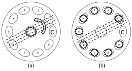
A polarized Monte Carlo program developed by Ra-mella-Roman et al. is at the core of our computational approach. Details of the basic algorithm and its validation are available in previous publications [24, 35]. Three different types of Monte Carlo programs were introduced in those publications, and in this paper the Meridian Planes Monte Carlo is utilized. The Meridian plane definition is given in the Section 2.1.1. Two major modifications are included: the ability to handle a medium exhibiting directional anisotropy and a geometrical arrangement of out-of-plane photon launching and detection. By out-of-plane, we mean a geometry where source, sample and detector do not lie uniquely in one reference plane, but vary sequentially. This approach is ultimately used to find the directional preference of the birefringent media without rotation of the sample or illumination polarizer, which is necessary for an in-plane scenario. Other studies were also conducted with what we refer to as “in-plane” geometry. This methodology is similar to what was initially proposed by Wang et al. [25]. In this arrangement the light source and detecting arm are in one plane consisting of sample. Figure 1 shows a top view of the in-plane (a) and out-of-plane (b) detection geometries. Dotted lines show the extraordinary axes of a sample with directional anisotropy. Detection of light back reflected from the sample could be performed while the sample is being rotated at different angles and illuminated with linearly polarized light in normal direction. For the out-of-plane measurement, the sample is in a fixed position and is illuminated sequentially by linearly polarized light by the illuminators at various azimuth angles.

Figure 1.

Top view geometry of the in-plane (a) and the out-of-plane (b) detection. Letter C indicates the location of the detection arm.

Scattering anisotropy of some particles and directional anisotropy of a birefringence medium could alter the measured state of polarization with respect to a reference polarizer. Scattering from particles in the Mie regime can change the status of polarization of impinging light from linearly into elliptically polarized [25, 36, 37]. For spherical particles, the elements of the scattering matrix depend on the particle size, scattering direction (scattering angle), and wavelength of the light. The refractive index in a birefringence medium is higher along its longitudinal direction than its transverse direction. Therefore, this anisotropic property yields a difference between the speeds of the cross- and co-polarized component of polarized light traveling inside a birefringence medium and can cause ellipticity. In this study, we consider the effect of both scattering and directional anisotropy of a birefringent turbid material on the state of polarization of propagating linearly polarized light. The birefringent effect of a highly scattering medium is analyzed by looking at the cyclical response of the degree of circular polarization (DOCP). Previous studies have shown that polarization properties of directional anisotropy of a medium can be modeled as linear birefringence [13, 26, 38, 39]. In the Monte Carlo framework a change in polarization of light travelling through a medium with linear birefringence can be expressed by modifying the related Stokes vector using the retardation Mueller matrix. Since birefringence of biological tissue tends to be small, its effect on the scattering phase function is often neglected [25, 26].

2.1.1 Handling a birefringent structure

Figure 2 shows the schematic of the problem in the Meridian planes [40]. The photon positions, before and after scattering, are represented as points A and B respectively. Each photon direction is uniquely described by two angles. The first angle is the angle between the initial photon direction and the Z-axis. The second angle is the angle between the Meridian plane and the X-Z-plane. The photon direction is also specified by a unit vector I₁ whose elements are specified by the direction cosines 〈u_x, u_y, u_z〉. The directions before and after scattering are called respectively I₁ and I₂. The unit vector I₁ and the Z-axis determine a plane COA. The COA plane is the Meridian plane. The incident field can be decomposed into two orthogonal components E_‖ and E_⊥, that describe the vibration of the electrical field parallel and perpendicular to the meridian plane. The sample is considered as a uniaxial birefringent material, the refractive indices of the medium differs along the extraordinary (n_e) and ordinary axes (n_o), both parallel to the X-Y-plane. Also, the birefringent effect is assumed to be coherent all around the sample. This means that the birefringence and its direction is the same for different positions inside the sample, although the model enables changes of the birefringence and angle of anisotropy to any number between two adjacent scattering events. The direction of the extraordinary axis is defined in the Monte Carlo algorithm with the angle of η, shown in Figure 2. Also σ is the angle between the projection of the E_‖ on the X-Y-plane and the extraordinary axis of the birefringent medium.

Figure 2.

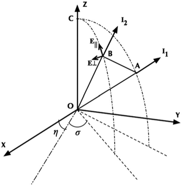
Schematic of the scattering problem of a birefringent structure in the Meridian planes.

The polarization of the field relative to the Meridian plane is described by a Stokes vector, S. When scattering occurs in the program, the Stokes vector reference plane needs to be altered properly. This is done by updating the Stokes vector with two rotations in and out of the scattering plane [24]. The polarization effect of directional anisotropy of the medium is considered between each scattering event by applying a retardation Mueller matrix.

Birefringence (Δn) is the maximum difference between the indices of refraction of the extraordinary (n_e) and ordinary axis (n_o). Δn = n(θ) – n_o where n(θ) is maximum refractive index seen by the photon propagating in the direction of θ with respect to the extraordinary axis of birefringent material and is given by [41]:

$$n(\theta )=\frac{n_o{n}_e}{{(n_e^2{cos}^2\theta +n_o^2{sin}^2\theta )}^{0.5}}$$ (1)

θ is calculated using the scalar product of the photon propagation direction and the extraordinary axis vector and can be written as:

$$\theta ={cos}^{-1}\left(\frac{u_{x}cos\eta +u_{y}sin\eta }{{(u_x^2+u_y^2+u_z^2)}^{0.5}}\right)$$ (2)

Using the last two equations, birefringence can be derived for each step of the photon propagation inside the medium. Consequently, the retardation, Δ is determined by:

$$\mathrm{\Delta }=\frac{2\mathrm{\pi }s\mathrm{\Delta }n}{\lambda }$$ (3)

where, s is the photon step size and λ is the photon wavelength. Furthermore, the retardation Mueller matrix can be written as [41, 42]:

$${\mathit{M}}_{\mathrm{\Delta }}=\left[\begin{array}{cccc}1& 0& 0& 0\\ 0& 1& 0& 0\\ 0& 0& cos\mathrm{\Delta }& sin\mathrm{\Delta }\\ 0& 0& -sin\mathrm{\Delta }& cos\mathrm{\Delta }\end{array}\right]$$ (4)

The above formalism is only valid when the horizontal component of the electric field is parallel to the extraordinary axis of the retarder. So, it is important to handle this issue by proper rotation of the polarization reference plane for the traveling photon after each scattering event. Defining the photon position based on the Meridian plane after each scattering event (COB in Figure 2), provides the angle ξ between the E_‖ and the X-axis. The projection vector of the E_‖ on the X-Y-plane is easily found from the photon direction cosines: 〈u_x, u_y, 0〉. Then ξ can be written as:

$$\xi =atan\left(\frac{u_y}{u_x}\right)$$ (5)

The angle σ can be calculated by knowing η and ξ. Therefore, the rotation Mueller matrix can be written as [41, 42]:

$$\mathit{R}(\sigma )=\left[\begin{array}{cccc}1& 0& 0& 0\\ 0& cos2\sigma & sin2\sigma & 0\\ 0& -sin2\sigma & cos2\sigma & 0\\ 0& 0& 0& 1\end{array}\right]$$ (6)

A precise rotation of the Stokes vector of the scattered photon by the angle σ is necessary before applying the retardation Mueller matrix to the Stokes vector. Ultimately as the photon continues its travel in the scattering medium a second rotation of −σ is necessary. Considering Stokes vector and Mueller matrix multiplication [42], the Stokes vector of the scattered photon passing through the birefringent medium can be updated as:

$${\mathit{S}}^{\text{'}}=\mathit{R}(-\sigma ){\mathit{M}}_{\mathrm{\Delta }}\mathit{R}(\sigma )\mathit{S}$$ (7)

In summary, the extended polarized Monte Carlo algorithm updates the Stokes vector of the photon at each moving step through the medium, based on the following relation:

$${\mathit{S}}^{\text{'}}=\mathit{R}(-\sigma ){\mathit{M}}_{\mathrm{\Delta }}\mathit{R}(\sigma )\mathit{R}(-\gamma )\mathit{M}(\alpha )\mathit{R}(\beta )\mathit{S}$$ (8)

where, M(α) is the single scattering matrix concluded from Mie theory [42], α is the scattering angle and β and γ are the rotation angles in and out of the scattering plane, respectively. All these parameters are well defined in Ref. [24].

The inclusion of birefringent structures in Monte Carlo program has been implemented by other groups [26, 27], in the result section of this paper we will compare the results of our model to the one published by Wood et al. [26]. Further validation that includes different launching and collection geometries will be also illustrated.

2.1.2 Out-of-plane geometry

The out-of-plane geometry is at the core of the proposed methodology for the quantification of a birefringent material preferential direction. Some changes to the original code were implemented to handle the new geometry as described in Figure 3. The photon direction cosines 〈u_x, u_y, u_z〉 were initialized to point to various non normal angles with respect to the sample surface. Considering the incident polar angle θ_i and the incident azimuth angle φ_i, the direction cosines are initialized as:

Figure 3.

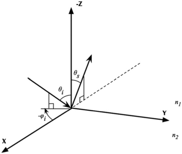
Schematic of the out-of-plane scattering implemented in the extended polarized Monte Carlo.

$$\begin{array}{c}{u}_x=-sin({\theta }_i)cos({\phi }_i)\\ u_y=-sin({\theta }_i)sin({\phi }_i)\\ u_z=cos({\theta }_i)\end{array}$$ (9)

The Fresnel effect of the boundary between surrounding medium and sample is neglected in this formalism.

The backscattered photons from the sample are collected at the scattered polar angle θ_s. In this study θ_i and θ_s are fixed while φ_i is allowed to change at initialization between 0 and 360 degrees.

2.2 Experimental setup

2.2.1 Out-of-plane polarimeter

An imaging system previously developed by our group to investigate rough surface scattering was utilized for this study [8, 43].

The out-of-plane system was equipped with nine light illumination ports (IP) all positioned at one incidence angle θ_i = 49 degree and nine different azimuth angles evenly spaced between 0 to 360 degrees (φ_i = 0, 36, 72, 108, 144, 216, 252, 288, and 324 degrees), Figure 4. The choice of these angles was simply made by attempting to cover available space of the imaging setup with the maximum number of IPs. Each IP contained a high performance white Light Emitting Diodes (Cree, Durham, NC) followed by a polarizer P2 (Edmund Optics, Barrington, NJ), and a lens L2 (Edmund Optics, Barrington, NJ). All IP components were embedded inside an illuminating tube to create a semi-collimated 2 cm diameter beam with fluence rate of approximately 2 [W cm^–2]. All IPs were controlled with a data acquisition (DAQ) module (National Instruments Corporation, Austin, TX). The out-of-plane illumination polarizers were aligned precisely at 45 degree with respect to the plane of incidence [43].

Figure 4.

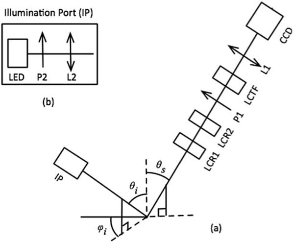
Schematic of the polarized light imaging arrangement (a) and the illumination port (b).

An imaging arm containing a Stokes polarimeter was positioned at a scattering angle θ_s = 49 degree, and φ_i = 180 degree. The imaging arm included two liquid crystal variable retarders (LCR1 and LCR2) (Meadowlark Optics Inc., Frederick, CO) followed by a liquid crystal tunable filter (LCTF) (Meadowlark Optics Inc., Frederick, CO) with a built-in vertical linear polarizer, P1. The LCR cells were mounted on manual rotational stages (precision of 1 degree) to precise adjustment of their ordinary axis.

The LCTF gives the ability to study multiple wavelengths with minor instrumentation adjustments. The LCTF range is 450 nm to 700 nm with the Full Width at Half Maximum (FWHM) of 7 nm. Wavelength of 632 nm was chosen for this study. A particular calibration technique described in Ref. [8] was used to correctly handle the wavelength dependent polarization properties of the instrument optics. Stokes vector images were captured using a fast acquisition black-and-white CCD camera (Teledyne Dalsa, Billerica, MA) connected to a zoom lens L1 (Computar, Commack, NY). A 1951 USAF chart target (Edmunds Industrial Optics, Barrington, NJ) was placed in the field of view of the imaging system to measure the detection resolution. The Stokes intensity image of the target was captured at 632 nm and an approximate value of 570 PPI (Pixel Per Inch) was calculated as imaging resolution.

Biological samples were positioned in a plastic container attached to a computerized rotational stage (Thorlabs, Newton, NJ). This rotating holder enabled the alignment of the sample surface parallel to the system reference plane as well as precise angular positioning of the sample.

Considering the Stokes vector S = [i, q, u, v], the degree of circular polarization, DOCP, can be calculated as v/i. We summarize the various computational and experimental approaches in Table 1.

Table 1.

Summary of computational and instrumentation geometries.

Layout	θi	θs	φi	Polarization	Experimental
In-plane/transmission	0°	180°	0°	Circular	Ref. [26]
Out-of-plane/reflection	49°	49°	0°–180°	Linear (45°)	Bovine leg Tendon

2.2.2 Biological sample

Tendon is a highly packed structure of birefringent collagen fibers and is a proper choice for this study. The dry mass of tendon contains about 86% collagen of which 98% is type I [44]. For this study, freshly excised bovine leg tendon tissue was obtained from a local supermarket. Fat and sheath layers were removed from the samples. For each experiment a section of approximately 3 cm × 1 cm × 0.5 cm (L × W × H) was used and positioned onto a rotary holder, no other material was added to the sample.

In order to model the experimental scenario described above, bovine tendon was modelled as a combination of scattering source (spherical scatterers with diameter of 0.3 μm) and a homogenous birefringence material (Δn = 2 × 10⁻⁴). This approach is similar to what proposed by others [25, 26, 45]. Birefringence of biological tissue is generally small (<0.01) [25, 26] and biological scatterers are often considered spherical with diameter ranging from 0.2 μm to 1.0 μm [45]. The Index of refraction of the scattering particles was chosen to be 1.4, which is the average value for various bovine tissues [46]. Since water is the major component of biological tissue, index of refraction of the background medium was set to 1.33. Index of refraction of the ordinary axis of the birefringent material was also set to the background value. Using our recently developed spatial frequency domain imaging system [43], scattering coefficient and absorption coefficient of the samples were calculated to be ∼24 cm⁻¹ (+/−3 cm⁻¹) and ∼1 cm⁻¹ (+/−0.1 cm⁻¹), respectively. The number of photons used in all simulations was 10⁷.

3. Results and discussion

3.1 Monte Carlo validation: In-plane geometry, transmission

In Ref. [26], Wood et al. have provided all information necessary to reproduce their tests. To validate the model performance, similar tests were performed using our model. Our Monte Carlo results and their experimental and computational results are shown in Figure 5. The calculated Root Mean Square Error for μ_s = 30 cm⁻¹ was 0.062 (Wood's value was 0.058), and for the case μ_s = 60 cm⁻¹ was 0.024 (Wood's value was 0.025).

Figure 5.

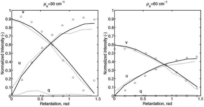
Monte Carlo simulations of an incident circularly polarized light beam through a slab of scattering acrylamide phantom (μ_s = 30 cm⁻¹ left and μ_s = 60 cm⁻¹ right). Empty symbols are experiments conducted by Wood et al. [26]. Solid lines are Wood's Monte Carlo simulations. Dashed lines are our Monte Carlo simulations.

The relevant terms used for the simulations were extracted and extrapolated from Wood's figures. The results are in excellent agreement with Wood's work, particularly when comparing both Monte Carlo programs (the RMSE for Monte Carlo results is 0.034 for μ_s = 30 cm⁻¹, and RMSE was 0.017 for μ_s = 60 cm⁻¹).

3.2 Monte Carlo simulations: Out-of-plane geometry, reflection

The sample under study consists of collagen fibers aligned relatively parallel to the longitudinal tendon axis. Therefore, a birefringent medium is simulated here with extraordinary axes oriented parallel to each other and for simplicity parallel to the air/medium of the sample. Figure 6 shows the results of the model for an out-of-plane measurement from the simulated birefringent medium. The relative orientation of the extraordinary axis (angle of η) is fixed with respect to the reference plane of the model. Two different orientations of extraordinary axis were modelled; 0 and 45 degrees. The DOCP reaches its minimum value once the azimuth angle of illumination coincides with the direction of the sample extraordinary axis. Therefore by detecting minimum of the DOCP graph, a quick assessment of the bundle directionality can be obtained.

Figure 6.

Out-of-plane polarized Monte Carlo: Degree of circular polarization versus incidence azimuth angle. Results are shown for two different orientations of extraordinary axis; η = 0 and 45 degrees.

3.3 Experiments on tendon: Out-of-plane geometry, reflection

An ex-vivo test on bovine tendon samples was conducted using the available out-of-plane polarized light imaging system. Stokes images of the light reflected from the sample at different azimuth angles were captured sequentially. DOCP showed a cyclic behavior dependent on the incidence azimuth angles, Figure 7 (left). In this figure, DOCP of a bovine tendon for two different positions are demonstrated. DOCP reached its minimum at azimuth angles of 0 (180) and 108 (288) degrees, which suggests the preferential orientation of collagen fibers. So once again, by quantifying the minimum of the DOCP graph, an assessment of the bundle extraordinary axis orientation was obtained for different examinations. All experiments were repeated three times the averaged standard deviation of the measurements over nine incident azimuth angles was ∼0.01. In Figure 7 (right) collagen orientation maps for these two samples are shown. The orientation maps were generated by finding the best fit between Monte Carlo result and the experimental data for each pixel of DOCP images. A least-square fitting algorithm based on the Nelder-Mead simplex minimization method [47] was applied here using Matlab (MathWorks, Natick, MA).

Figure 7.

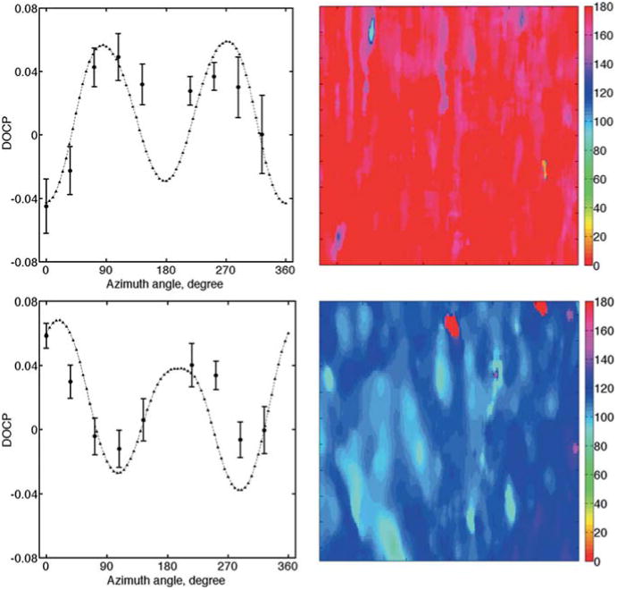
Out-of-plane polarized light imaging: DOCP versus incidence azimuth angle for a bovine leg tendon positioned at 0 and 108 degrees (left graphs). Circles show the average DOCP over the ROI. The error bars represent the standard deviation of the data. Triangles show the Monte Carlo prediction. Right maps show the corresponding collagen orientation maps for an area of 2 by 5 millimeter.

A summary of the results for several experiments is ultimately shown in Figure 8.

Figure 8.

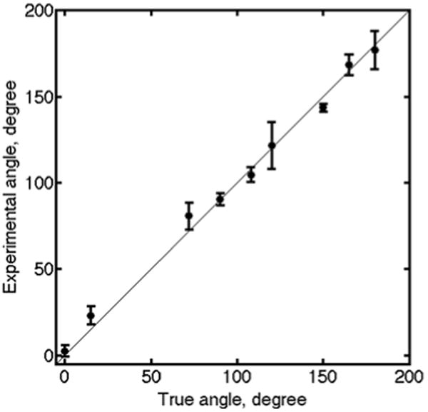
Out-of-plane experiments were performed on bovine leg tendons with extraordinary axis positioned at different known angles η (0, 15, 72, 90, 108, 120, 150, 165, and 180 degrees). Circles show the average detected experimental angle over the ROI. The error bars represent the standard deviation of the data.

4. Conclusion

In this paper, we demonstrated a new out-of-plane theoretical and non-invasive experimental approach aimed at assessing the directional anisotropy of a highly scattering medium. In this approach the extraordinary axis of the birefringent material was quantified simply by observing the angle, which DOCP reaches its minimum value. Furthermore, since no angular rotation of the sample or changes in the illumination polarization is required, and the experiment is conducted in reflectance, the out-of-plane method seems to be relatively easier to implement than more traditional in-plane techniques specifically for biological in-vivo applications.

A Monte Carlo model of polarized light transfer into multiply scattering medium was also extended to handle birefringent materials exhibiting directional anisotropy. The Stokes vector associated with a traveling photon was updated between each scattering event not only to handle scattering but also the retardation properties of the material. The degree of circular polarization of the backscattered light is shown to be a sensitive marker for the investigation of directional anisotropy. Tests conducted on collagenous samples confirmed the model results.

Analysis of DOCP of the light reflected from a tendon sample for different incidence azimuth angles yields informative maps of the preference directionality of the collagen fibers. Oscillatory behavior of DOCP is seen due to the constructive or destructive coincidence of the birefringence direction and the incident linearly polarized light.

Although further testing in different birefringent samples needs to be performed to confirm the validity of this approach, we believe that this technique will be useful in monitoring tissue birefringent structural alignment.

In the model a number of approximations were made, firstly the scatterers in the biological medium were considered spherical particles; the birefringence of the medium was set as homogeneous with orientation and magnitude fixed at each position. Furthermore the birefringent material main axes were assumed to be parallel to the surface. As we extend this work to more complex tissues we plan to improve on the proposed model to include layered structure to mimic biological tissue more accurately.

References

- 1.Oldenbourg RA. Nature. 1996;381(2):811–812. doi: 10.1038/381811a0. [DOI] [PubMed] [Google Scholar]
- 2.Jacques SL, Ostermeyer M, Wang L, Stephens D. Proc SPIE. 1996;2671:199–210. [Google Scholar]
- 3.Groner W, Winkelman JW, Harris AG, Ince C, Bouma GJ, Messmer K, Nadeau RG. Nat Med. 1999;5(10):1209–1212. doi: 10.1038/13529. [DOI] [PubMed] [Google Scholar]
- 4.Jacques SL, Ramella-Roman JC, Lee K. Lasers Surg Med. 2000;26(2):119–129. doi: 10.1002/(sici)1096-9101(2000)26:2<119::aid-lsm3>3.0.co;2-y. [DOI] [PubMed] [Google Scholar]
- 5.Jacques SL, Ramella-Roman JC, Lee K. J Biomed Opt. 2002;7(3):329–340. doi: 10.1117/1.1484498. [DOI] [PubMed] [Google Scholar]
- 6.Ramella-Roman JC, Lee K, Prahl SA, Jacques SL. J Biomed Opt. 2004;9(6):1305–1310. doi: 10.1117/1.1781667. [DOI] [PubMed] [Google Scholar]
- 7.Antonelli MR, Pierangelo A, Novikova T, Validire P, Benali A, Gayet B, De Martino A. Opt Express. 2010;18(10):10200–10208. doi: 10.1364/OE.18.010200. [DOI] [PubMed] [Google Scholar]
- 8.Ghassemi P, Lemaillet P, Germer TA, Shupp JW, Venna SS, Boisvert ME, Flanagan KE, Jordan MH, Ramella-Roman JC. J Biomed Opt. 2012;17(7):076014. doi: 10.1117/1.JBO.17.7.076014. [DOI] [PMC free article] [PubMed] [Google Scholar]
- 9.Kunnen B, Macdonald C, Doronin A, Jacques S, Eccles M, Meglinski I. J Biophotonics. 2014 doi: 10.1002/jbio.201400104. [DOI] [PubMed] [Google Scholar]
- 10.de Boer JF, Milner TE, van Gemert MJC, Stuart Nelson J. Opt Lett. 1997;22(12):934–936. doi: 10.1364/ol.22.000934. [DOI] [PubMed] [Google Scholar]
- 11.Yang Y, Rupani A, Bagnaninchi P, Wimpenny I, Weightman A. J Biomed Opt. 2012;17(8):081417. doi: 10.1117/1.JBO.17.8.081417. [DOI] [PubMed] [Google Scholar]
- 12.Pierce MC, Sheridan RL, Hyle Park B, Cense B, de Boer JF. Burns. 2004;30(6):511–517. doi: 10.1016/j.burns.2004.02.004. [DOI] [PubMed] [Google Scholar]
- 13.Oh JT, Lee SW, Kim YS, Suhr KB, Kim BM. J Biomed Opt. 2006;11(4):041124–041127. doi: 10.1117/1.2338826. [DOI] [PubMed] [Google Scholar]
- 14.Jiao S, Wang LV. Opt Lett. 2002;27(2):101–103. doi: 10.1364/ol.27.000101. [DOI] [PubMed] [Google Scholar]
- 15.Götzinger E, Pircher M, Baumann B, Ahlers C, Geitzenauer W, Hitzenberger W, Schmidt-Erfurth U, Hitzenberger CK. Opt Express. 2009;17(5):4151–4165. doi: 10.1364/oe.17.004151. [DOI] [PMC free article] [PubMed] [Google Scholar]
- 16.Duan L, Marvdashti T, Lee A, Tang JY, Ellerbee AK. Biomed Opt Express. 2014;5(10):3717–3729. doi: 10.1364/BOE.5.003717. [DOI] [PMC free article] [PubMed] [Google Scholar]
- 17.Wu PJ, Walch JT., Jr J Biomed Opt. 2005;37(5):396–406. [Google Scholar]
- 18.Wu PJ, Walch JT., Jr J Biomed Opt. 2006;11(1):014031. doi: 10.1117/1.2162851. [DOI] [PubMed] [Google Scholar]
- 19.Wood MF, Ghosh N, Wallenburg MA, Li SH, Weisel RD, Wilson BC, Li RK, Vitkin IA. J Biomed Opt. 2010;15(4):047009. doi: 10.1117/1.3469844. [DOI] [PubMed] [Google Scholar]
- 20.Alali S, Aitken KJ, Schröder A, Bagli DJ, Vitkin IA. J Biomed Opt. 2012;17(8):086010. doi: 10.1117/1.JBO.17.8.086010. [DOI] [PubMed] [Google Scholar]
- 21.Vidal BC. Micron. 2003;34(8):423–432. doi: 10.1016/S0968-4328(03)00039-8. [DOI] [PubMed] [Google Scholar]
- 22.Aro AA, Freitas KM, Freitas KM, Foglio MA, Carvalho JE, Dolder H, Gomes L, Vidal BC, Pimentel ER. Life Sci. 2013;S0024-3205(13):00116–1. doi: 10.1016/j.lfs.2013.02.011. [DOI] [PubMed] [Google Scholar]
- 23.Riberio JF, dos Anjos EHM, Mello MLS, Vidal BD. PLoS One. 2013;8(1):e54724. doi: 10.1371/journal.pone.0054724. [DOI] [PMC free article] [PubMed] [Google Scholar]
- 24.Ramella-Roman JC, Prahl SA, Jacques SL. Opt Express. 2005;13(12):4420–4438. doi: 10.1364/opex.13.004420. [DOI] [PubMed] [Google Scholar]
- 25.Wang W, Wang LV. J Biomed Opt. 2002;7(3):350–358. doi: 10.1117/1.1483878. [DOI] [PubMed] [Google Scholar]
- 26.Wood MFG, Guo X, Vitkin A. J Biomed Opt. 2007;12(1):014029. doi: 10.1117/1.2434980. [DOI] [PubMed] [Google Scholar]
- 27.Cameron BD, Raković MJ, Mehrübeoglu M, Kattawar GW, Rastegar S, Wang LV, Coté GL. Optics Letters. 1998;23(7):485–487. doi: 10.1364/ol.23.000485. [DOI] [PubMed] [Google Scholar]
- 28.Wallenburg MA, Wood MF, Ghosh N, Vitkin IA. Optics Letters. 2010;35(15):2570–2572. doi: 10.1364/OL.35.002570. [DOI] [PubMed] [Google Scholar]
- 29.Raković MJ, Kattawar GW, Mehrübeoglu M, Cameron BD, Wang LV, Rastegar S, Coté GL. Applied Optics. 1999;38(15):3399–3408. doi: 10.1364/ao.38.003399. [DOI] [PubMed] [Google Scholar]
- 30.Yao G, Wang LV. Opt Express. 2000;7(5):198–203. doi: 10.1364/oe.7.000198. [DOI] [PubMed] [Google Scholar]
- 31.Wang X, Wang LV, Sun CW, Yang CC. J Biomed Opt. 2003;8(4):608–617. doi: 10.1117/1.1606462. [DOI] [PubMed] [Google Scholar]
- 32.Côté D, Vitkin IA. Opt Express. 2005;13(1):148–163. doi: 10.1364/opex.13.000148. [DOI] [PubMed] [Google Scholar]
- 33.Gangnus SV, Matcher SJ, Meglinski IV. Proc SPIE. 2002;4619:281–288. [Google Scholar]
- 34.Wang X, Yoa G, Wang LV. Appl Opt. 2002;41(4):792–801. doi: 10.1364/ao.41.000792. [DOI] [PubMed] [Google Scholar]
- 35.Ramella-Roman JC, Prahl SA, Jacques SL. Opt Express. 2005;13(25):10392–10405. doi: 10.1364/opex.13.010392. [DOI] [PubMed] [Google Scholar]
- 36.Wang X, Yao G, Wang LV. Appl Opt. 2002;41(4):792–801. doi: 10.1364/ao.41.000792. [DOI] [PubMed] [Google Scholar]
- 37.Tuchin VV. Physics-Uspekhi. 1997;40(5):495–515. [Google Scholar]
- 38.Alali S, Wang Y, Vitkin A. Biomed Opt Express. 2012;3(12):3250–3263. doi: 10.1364/BOE.3.003250. [DOI] [PMC free article] [PubMed] [Google Scholar]
- 39.De Boer JF, Milner TE. Biomed Opt Express. 2002;7(3):359–371. doi: 10.1117/1.1483879. [DOI] [PubMed] [Google Scholar]
- 40.S. Chandrasekhar, Oxford Clarendon Press (1950).
- 41.Saleh BEA, Teich MC. Wiley-Interscience. 1991;Chap. 6 [Google Scholar]
- 42.Bohren C, Huffman DR. Wiley Science Paperback Series. 1998 [Google Scholar]
- 43.Ghassemi P, Travis TE, Moffatt LT, Shupp JW, Ramella-Roman JC. Biomed Opt Express. 2014;5(10):3337–3354. doi: 10.1364/BOE.5.003337. [DOI] [PMC free article] [PubMed] [Google Scholar]
- 44.Woo SL, An KN, Frank CB. In: editor Orthopaedic Basic Science. Simon R, editor. Rosemont: AAOS; 2000. pp. 581–616. [Google Scholar]
- 45.Mourant JR, Freyer JP, Hielscher AH, Eick AA, Shen D, Johnson TM. Appl Opt. 1998;37(16):3586–3593. doi: 10.1364/ao.37.003586. [DOI] [PubMed] [Google Scholar]
- 46.Bolin FP, Preuss LE, Taylor RC, Ference RJ. Appl Opt. 1989;28(12):2297–2303. doi: 10.1364/AO.28.002297. [DOI] [PubMed] [Google Scholar]
- 47.Nelder JA, Mead R. Comp J. 1965;7(4):308–313. [Google Scholar]