Spatial Big Data Analytics of Influenza Epidemic in Vellore, India

Abstract

The study objective is to develop a big spatial data model to predict the epidemiological impact of influenza in Vellore, India. Large repositories of geospatial and health data provide vital statistics on surveillance and epidemiological metrics, and valuable insight into the spatiotemporal determinants of disease and health. The integration of these big data sources and analytics to assess risk factors and geospatial vulnerability can assist to develop effective prevention and control strategies for influenza epidemics and optimize allocation of limited public health resources. We used the spatial epidemiology data of the HIN1 epidemic collected at the National Informatics Center during 2009-2010 in Vellore. We developed an ecological niche model based on geographically weighted regression for predicting influenza epidemics in Vellore, India during 2013-2014. Data on rainfall, temperature, wind speed, humidity and population are included in the geographically weighted regression analysis. We inferred positive correlations for H1N1 influenza prevalence with rainfall and wind speed, and negative correlations for H1N1 influenza prevalence with temperature and humidity. We evaluated the results of the geographically weighted regression model in predicting the spatial distribution of the influenza epidemic during 2013-2014.

I. Introduction

The continuing challenge in global public health surveillance is to determine the risk posed by the infectious disease outbreaks with improved understanding of their natural geographic range. The size of the spatial epidemiology data grows large and utilization of useful intelligence in these data has become a priority. They share similar big data characteristics of volume, velocity, variety, value and veracity [1]. The spatial epidemiology data constitutes a keystone of big data and health analytics challenges in digital epidemiology [2]. This study analyzes the spatial big data challenges in infectious disease surveillance, with a focus on influenza epidemics.

A. Mathematical Models of Infectious Disease Epidemics

Mathematical models play a major role in understanding and predicting the spatiotemporal dynamics of infectious disease epidemics, and assisting in improving prevention and control policies and practices [3-6]. Bayesian networks technique is applied to model the spatio-temporal patterns of a non-contagious disease (respiratory anthrax infection) in a sample population [7-9]. Kulldroff used a spatial cluster method to group the disease cases based on location [10]. Spatial movement of individuals between locations and their contacts are monitored, grouped and visualized to control the disease spread [11].

B. Spatial Analytics of Infectious Disease Epidemics

Chi et al. summarize the application of statistical models for spatial data analysis and spatial regression modeling in population dynamics [12]. Buscema et al. applied topological weighted centroid method to predict the outbreak of Escherichia coli [13]. While the predicted results depend on the specific properties of the dataset, the parameters used to determine the utility of the predictor function are sample size, sample configuration, sample variation, distribution shape, spatial heterogeneity and spatial autocorrelation.

C. Influenza Epidemiology in Vellore, India

The influenza H1N1 epidemic initiated at Mexico in March 2009, and spread globally. The influenza surveillance program in India monitored for patients with influenza symptoms. Symptoms include fever, nasal discharges, cough, headache, sore throat and respiratory problems. 10,193 cases were confirmed, with a large proportion of patients in South India, especially in Vellore. Vellore district had a high incidence of H1N1 cases, with dynamic population moving in and around Vellore. There were 433 cases reported officially; due to under-reporting, there is likely to be more than 100,000 cases that were not reported.

D. Public Health Significance

In this study, we have developed an ecological niche model based on geographically weighted regression for predicting influenza epidemiological impact in Vellore during 2013-2014, using the spatial epidemiology and ecological data of the 2009-2010 HIN1 epidemic collected at the National Informatics Center in Vellore.

II. Methods

A. Spatial Autocorrelation

Tobler's first law of geography (TFL) states “Everything is related to everything else, but near things are more related than distant things” [14-15]. Spatial autocorrelation factor is used to estimate the trueness of the Tobler’s law by determining the correlation of a variable with itself over space [14, 16]. Moran’s I is a statistical measure of spatial autocorrelation [17-18]. The variations of Moran’s I include Global Moran’s I and Local Moran’s I. Global Moran’s I is used to measure the spatial autocorrelation of the entire global region and Local Moran’s I is used to measure the spatial autocorrelation for each local region. Spatial autocorrelation at the local region has been used in infectious disease surveillance of dengue, HIV/AIDS and influenza to identify the hot spot locations of high disease incidence and prevalence [19-21].

B. Clustering by Hot Spot - Cold Spot Analysis

Spatial distribution of H1N1 cases are statistically calculated and clustered by Getis-Ord G statistics. It groups the spatial distribution of disease prevalence in terms of high values and low values. Clustering of high disease prevalence is referred as hotspots and clustering of low disease prevalence is referred as cold spots [22]. The hot spots and cold spots of HIN1 cases are clustered based on G score values. The computations of Getis-Ord G statistics, including the expected value are shown below.

$$G_i^{\ast }=\frac{{\Sigma }_{j=1}^n{W}_{ij}\left(d\right)y_i}{{\Sigma }_{j=1}^n{y}_i}$$

$G_i^{\ast }$ = G Statistic value

W_ij = Weight matrix

d = Euclidean distance

y_j = Number of infected in each location

$$E\left(G_i^{\ast }\right)=W_i^{\ast }∕n$$

$$W_i^{\ast }={\Sigma }_{j=1}^n{W}_{ij}\left(d\right)$$

C. Prediction by Geographically Weighted Regression Model

Traditional regression models are focused on global parameters, but the Geographically Weighted Regression (GWR) model is used to estimate the local parameters. Non-stationarity models like the geographically weighted regression model account for modeling the different observations in different locations of the study area. The geographically weighted regression model generates regression coefficients that vary over space, by estimating a separate regression coefficient for each location. Parameter y_i denotes the prevalence of H1N1 cases in each location. It is calculated by summing up the past observations with dissimilar weights [23-24]. The model is represented as follows.

$$y_i={\beta }_0+{\beta }_1(A_i,B_i)+{\beta }_2(A_i,B_i)X_1+\dots +{\beta }_i(A_i,B_i)X_{ik}+{\epsilon }_{ik}$$

β_i(A_i, B_i) is a function of latitude and longitude coordinates of location i, and is calculated using weighted least square procedure. Specific coefficient can be calculated for each location i by,

β_i = Coefficient for each location i

A_i = Latitude

B_i = Longitude

$\widehat{\beta }\left(i\right)$ = [XⁱW(i)X]⁻¹X′W(i) i=1, 2,…, n

Spatial observations are weighted based on the Euclidean distance between the locations i and j. Weights W_ij are calculated using the distance function d_ij between the particular location i and other locations, as shown below.

$$W_{ij}=exp\left[-\left(\raisebox{1ex}{${d_{ij}}^2$}\!\left/ \!\raisebox{-1ex}{$b^2$}\right.\right)\right]$$

W_ij = Weight of the data point j at location i

d_ij = Distance between the locations and i and j

b = Bandwidth

Fig. 1 illustrates the geographically weighted regression model to predict the H1N1 influenza epidemic for 2013-2014 given the H1N1 prevalence and climatic data of August 2009 to July 2010. The geographically weighted regression model finds the local regression model for each region i, and uses the local regression coefficient to estimate the influenza prevalence for 2013-2014. Diagnostics block are used to validate our model based on the Akaike information criteria and R² value. Coefficient and prediction blocks are used to generate the predicted values. The results of the geographically weighted regression model are evaluated in terms of residuals and regression coefficient. The model and simulation is implemented in ArcGIS 10.0 [25].

Fig. 1. Geographically Weighted Regression Model of H1N1 Influenza Epidemic.

The geographically weighted regression model is calibrated using the H1N1 influenza prevalence and ecological data during 2009-2010, and used to predict the epidemiological impact of H1N1 influenza during 2013-2014.

III. Results

A. Study Area

The study area is Vellore district of Tamil Nadu state, which is located in southern India. The latitude and longitude for the Vellore district is 12.9202° N, 79.133° E. Fig. 2 depicts the prevalence of H1N1 influenza in each administrative division of Vellore district during August 2009 to July 2010.

Fig. 2. H1N1 influenza prevalence during August 2009-July 2010.

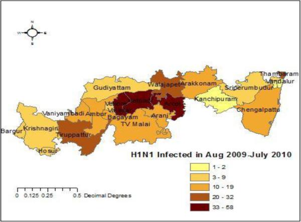
Prevalence of H1N1 influenza in each administrative division of Vellore district during August 2009-July 2010. Results show an outbreak in Katpadi, Arcot and Gudiyatham.

B. Climate Conditions

Climate condition attributes of temperature, humidity, wind speed and rainfall are collected division wise from the Vellore Agriculture Department for August 2009 to July 2010, as shown in Table I; population and H1N1 prevalence are also included in the table.

TABLE I.

Climate conditions in Vellore. Climate data are derived from the Vellore Agriculture Department to include the environmental parameters that may impact the H1N1 influenza epidemic.

FID	NAME_3	Infected	Temperature	Humidity	Windspeed	Rainfall	Population
0	Kelambakkam	6	24.56	64.21	6	63	23453
1	Thambaram	22	20.76	54.23	9	85	174787
2	Koyambedu	1	35.56	64.98	4	56	12323
3	Vandalur	1	35.24	63.45	4	59	13311
4	Krishnagiri	8	25.02	66.34	7	71	1879809
5	Chengalpattu	11	24.12	65.96	8	75	571254
6	Kanchipuram	2	35.23	63.23	5	62	3998252
7	Sriperumbudur	7	35.23	57.04	6	65	486063
8	Arani	14	28.43	63.12	9	79	63671
9	TV Malai	15	29.45	63.34	9	81	144278
10	Arakkonam	12	32.65	64.85	9	76	101626
11	Arcot	38	24.3	60.4	11	105	95955
12	Gudiyattam	9	33.56	65.34	8	74	91558
13	Tiruppattur	24	26.2	62.34	9	89	500455
14	Ambur	16	27.3	52.76	10	83	114608
15	Katpadi	43	22.3	58.57	12	112	387922
16	Walajapet	32	25.4	61.34	11	95	32397
17	Vaniyambadi	19	20.23	65.87	9	84	95061
18	Bagayam	12	22.12	53.32	8	75	23145
19	Vellore	58	20.3	65.01	13	124	177230
20	Vallalar	7	35.1	64.98	7	68	25092
21	Hosur	8	35.023	65.34	7	72	1879809
22	Bargur	5	35.22	63.3	5	63	1879809

C. Correlation Analysis using Scatter plots

Scatter plots are used to analyze the degree of correlation between temperature, humidity, wind speed, rainfall and population with H1N1 influenza prevalence, as shown in Fig. 3. We observed positive correlations between H1N1 influenza prevalence and rainfall, and between H1N1 influenza prevalence and wind speed. We observed negative correlations between H1N1 influenza prevalence and temperature, and between H1N1 influenza prevalence and humidity.

Fig. 3. Correlation analysis using scatter plots.

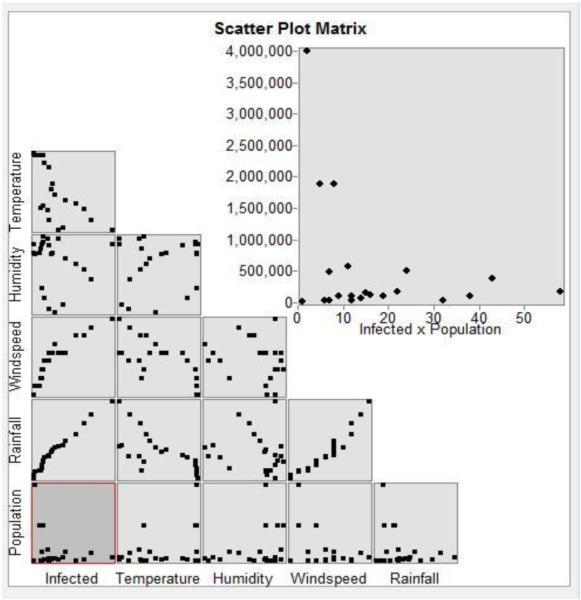
Analysis of the scatter plots infer that rainfall and windspeed have a positive correlation, whereas temperature and humidity have a negative correlation on H1N1 influenza prevalence.

D. Clustering by Hot Spot – Cold Spot Analysis

Fig. 4 depicts the hot spot and cold spot locations for the H1N1 epidemic during the winter season. The hot spot is observed in Arani and the cold spot in Sriperumbudur.

Fig. 4. H1N1 hotspot – cold spot analysis.

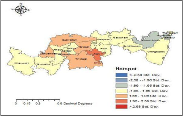
Arani is identified as the hot spot and Sriperumbuthur is identified to be a cold spot for H1N1 influenza.

E. Parameter Values

The values of the parameters used for prediction are shown in Table II.

TABLE II.

Parameters’ Estimation Using Ordinary Least Squares. Linear regression analysis of correlation between H1N1 influenza prevalence and rainfall, wind speed, humidity and temperature using ordinary least squares estimation method.

	Variable	Co-efficient	P value
OLS	Rainfall	0.2013	0.0012
	Wind speed	1.0232	0.0032
	Humidity	−1.0197	0.0234
	Temperature	−1.3423	0.0487
	R 2	0.924875
	Adjusted R2	0.914620
	AIC	124.5678

F. Residuals

The residuals measure the difference between the predicted and actual values using ordinary least squares. Fig. 5 shows the spatial distribution of the residuals. In order to validate the parametric values within the neighborhood, geographically weighted regression and spatial autocorrelation is applied. GWR spatial autocorrelation significance is shown in Table III and proves to have a correlation with the derived GWR model.

Fig. 5. Ordinary least squares residuals.

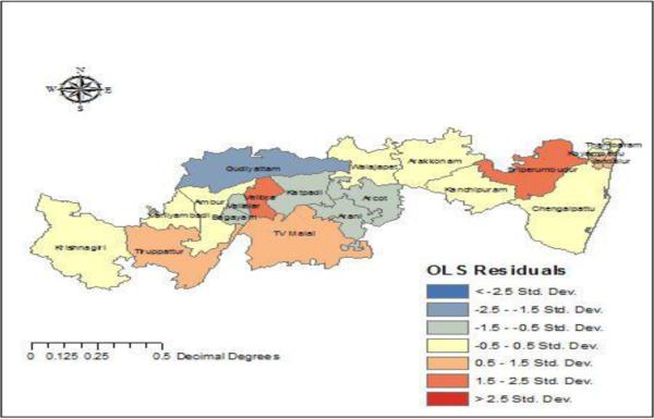
The spatial distribution of the residuals is mapped.

TABLE III.

Spatial autocorrelation for residuals in geographically weighted regression model. The p-value is statistically significant and the z-score is positive, thereby inferring spatial autocorrelation between the spatial locations and the feature values.

GWR	Moran’s Index	0.249226
	Expected Index	0.050000
	Variance Z score	0.009890
	Z score	1.003338
	P value	0.045141

G. Regression Coefficient Prediction

After identifying the correlations using data from 2009-2010, regression coefficients are used to predict the H1N1 prevalence in each location during 2013-2014. Regression coefficients are calculated and shown in Table IV and Table V.

TABLE IV.

Coefficient prediction for August 2009-July2010. The coefficients are predicted using the data from the 2009-2010 H1N1 influenza season.

FID	LocalR2	Predicted	Intercept	C2_Rainfall	C3_Wind	C1_Hum	C1_Temp
0	0.941536	4.272267	65.96521	0.20191	1.569884	−1.01122	−1.2123
1	0.941347	7.57038	65.8725	0.20017	1.57597	−1.01176	−1.20799
2	0.941604	7.218828	65.97145	0.201849	1.387915	−1.0117	−1.21268
3	0.941484	4.096468	65.89729	0.200351	1.474089	−1.01174	−1.20928
4	0.976791	7.394924	72.69193	0.399978	1.513415	−1.01295	−1.55314
5	0.94231	15.50616	66.18829	0.205244	1.390119	−1.01159	−1.22327
6	0.944341	5.702962	67.2873	0.227909	1.461877	−1.01125	−1.27439
7	0.942483	4.272507	66.45469	0.211483	1.55629	−1.01147	−1.23504
8	0.962413	13.89707	72.5177	0.339014	1.513841	−1.01297	−1.53259
9	0.968666	4.273444	73.07605	0.372021	1.570263	−1.01258	−1.56524
10	0.945692	12.46897	67.96397	0.242234	1.570797	−1.01119	−1.30589
11	0.954576	36.2268	70.6383	0.297585	0.62999	−1.01189	−1.43766
12	0.971071	8.998451	73.36439	0.383539	1.431956	−1.01276	−1.57934
13	0.975043	9.083651	72.81947	0.39311	1.583877	−1.01264	−1.55772
14	0.973581	5.962924	73.01804	0.389487	1.497208	−1.01253	−1.56559
15	0.967572	61.02714	73.34657	0.369609	1.451583	−1.0131	−1.57601
16	0.95332	15.50215	70.38698	0.292211	1.526968	−1.01177	−1.42401
17	0.974829	7.566075	72.92495	0.393613	1.426165	−1.01264	−1.56218
18	0.972607	4.273573	73.07329	0.386307	1.540191	−1.0125	−1.56748
19	0.970729	45.7655	73.24372	0.381163	1.26015	−1.01263	−1.57387
20	0.972231	7.394772	73.14261	0.385677	1.518715	−1.01253	−1.57031
21	0.97651	5.877111	72.65238	0.397816	1.494516	−1.01289	−1.55128
22	0.977283	2.671446	72.63378	0.40186	1.419994	−1.01307	−1.55091

TABLE V.

Predicted values of H1N1 influenza prevalence during 2013-2014. The epidemiological impact of H1N1 influenza during 2013-2014 is predicted by the geographic weighted regression model.

FID	LocalR2	Predicted	Intercept	C2_Rainfall	C3_Wind	C1_Hum	C1_Temp
0	0.941536	9.796861	65.96521	0.20191	1.569884	−1.01122	−1.2123
1	0.941347	11.67607	65.8725	0.20017	1.57597	−1.01176	−1.20799
2	0.941604	−0.92398	65.97145	0.201849	1.387915	−1.0117	−1.21268
3	0.941484	1.967236	63.39729	0.200351	1.474089	−1.01174	−1.20928
4	0.976791	4.567098	72.69193	0.399978	1.513415	−1.01295	−1.55314
5	0.94231	19.17416	66.18829	0.205244	1.390119	−1.01159	−1.22327
6	0.944341	1.003856	67.2873	0.227909	1.461877	−1.01125	−1.27439
7	0.942483	5.944097	66.45469	0.211483	1.55629	−1.01147	−1.23504
8	0.962413	13.78208	72.5177	0.339014	1.513841	−1.01297	−1.53259
9	0.968666	16.70506	73.07605	0.372021	1.570263	−1.01258	−1.56524
10	0.945692	13.87228	67.96397	0.242234	1.570797	−1.01119	−1.30589
11	0.954576	3.91911	70.6383	0.297585	0.62999	−1.01189	−1.43766
12	0.971071	5.358784	73.36439	0.383539	1.431956	−1.01276	−1.57964
13	0.975043	15.49282	72.31947	0.39311	1.583877	−1.01264	−1.55772
14	0.973581	21.45832	73.01804	0.389487	1.497208	−1.01253	−1.56559
15	0.967572	23.1736	73.34657	0.369609	1.451583	−1.0131	−1.57601
16	0.95332	18.11901	70.38698	0.292211	1.526968	−1.01177	−1.42401
17	0.974829	21.43777	72.92495	0.393613	1.426165	−1.01264	−1.56218
18	0.972607	7.055796	73.07329	0.386307	1.540191	−1.0125	−1.56748
19	0.970729	29.55596	73.24372	0.381163	1.26015	−1.01263	−1.57387
20	0.972231	13.92465	73.14261	0.385677	1.518715	−1.01253	−1.57031
21	0.97651	4.135098	72.65238	0.397816	1.494516	−1.01289	−1.55128
22	0.977283	1.119658	72.63378	0.40186	1.419994	−1.01307	−1.55091

The spatial distribution of the coefficient values for rainfall, temperature, wind speed and humidity are shown in Fig. 6, Fig. 7, Fig. 8 and Fig. 9 respectively.

Fig. 6. Rainfall coefficient.

Rainfall is positively correlated with the prevalence of H1N1 influenza. Areas around Chengalpatu has high rainfall coefficients compared to other locations, and the neighbourhood locations of Krishnagiri has lower rainfall coefficients.

Fig. 7. Temperature coefficient.

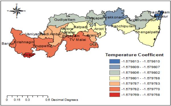
Temperature is negatively correlated with the prevalence of H1N1 influenza.TV Malai, Krishnagiri, Thirupattur has low temperature coefficients while Arakonam and Thambaram have high temperature coefficients.

Fig. 8. Windspeed coefficient.

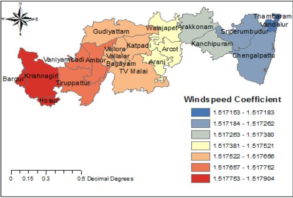
Windspeed is positively correlated with the prevalence of H1N1 influenza. Areas around Krishnagiri have high windspeed and areas near Thambaram have low windspeed.

Fig. 9. Humidity coefficient.

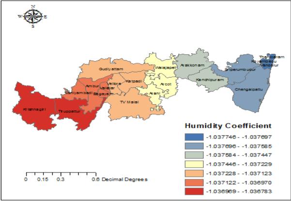
Humidity is negatively correlated with the prevalence of H1N1 influenza. Areas near Krishnagiri and Tirupattur have high humidity and Chengalpattu has low humidity.

The spatial distribution of H1N1 influenza prevalence is predicted for each location, and is shown in Fig. 10. The predictions for 2013-2014 are based on the regression coefficients estimated using the data from 2009-2010.

Fig. 10. Prediction of H1N1 influenza.

The spatial distribution of H1N1 infuenza prevalence for 2013-2014 is predicted.

IV. Discussion

We developed an ecological niche model based on geographically weighted regression method to predict the epidemiological impact of H1N1 influenza during 2013-2014 season. We integrated the spatial epidemiology data of H1N1 influenza prevalence and environmental data from 2009-2010 season. We inferred that H1N1 influenza prevalence has positive correlations with rainfall and wind speed, and negative correlations with temperature and humidity.

A. Limitations

The ecological niche model based on geographically weighted regression is used to predict the spatial distribution of H1N1 influenza prevalence. While the environmental variables of rainfall, wind speed, temperature and humidity correlate to the risk of influenza incidence and prevalence in different regions, biological and socio-behavioral attributes of H1N1 influenza transmission dynamics are not incorporated in the model.

B. Public Health Implications

The ecological niche model based on geographically weighted regression is used to predict the epidemiological impact of H1N1 influenza in different regions. Thereby, high risk areas for H1N1 influenza can be prioritized for implementation of prevention interventions.

C. Conclusion

Epidemiological models of infectious diseases are useful to predict the epidemiological morbidity and mortality, identify vulnerable populations, assess the beneficial impact of available interventions, compare different implementation options, and improve public understanding of infectious disease dynamics [26]. We presented the ecological niche model based on geographically weighted regression to predict the incidence and prevalence of H1N1 influenza in different regions of Vellore, India, thereby assisting in prioritizing high risk areas for implementation of optimal prevention interventions.

The integration of health, climate and environmental data, supported by geographical information systems and satellite imagery, and combined with computational tools facilitate the design and development of early warning systems for influenza epidemics, and can be adapted to control and prevent epidemics of other infectious diseases.

REFERENCES

- 1.Burke J. Health Analytics: Gaining the Insights to Transform Health Care. 1 Wiley; Hoboken, New Jersey: 2013. [Google Scholar]
- 2.Salathé M, Bengtsson L, Bodnar TJ, Brewer DD, Brownstein JS, Buckee C, Campbell EM, Cattuto C, Khandelwal S, Mabry PL, Vespignani A. Digital Epidemiology. PLoS Comput Biol. 2012;8(7):e1002616. doi: 10.1371/journal.pcbi.1002616. [DOI] [PMC free article] [PubMed] [Google Scholar]
- 3.Vynnycky E, White R. An Introduction to Infectious Disease Modelling. 1st Oxford University Press; USA: 2010. [Google Scholar]
- 4.Keeling MJ, Rohani P. Modeling Infectious Diseases in Humans and Animals. 1st Princeton University Press; 2007. [Google Scholar]
- 5.Pfeiffer DU, Robinson TP, Stevenson M, Stevens KB, Rogers DJ, Clements ACA. Spatial Analysis in Epidemiology. 2008. Also available as: Hardback | eBook.
- 6.Waller LA, Gotway CA. Applied Spatial Statistics for Public Health Data. 1 Wiley-Interscience; Hoboken, N.J: 2004. [Google Scholar]
- 7.Jiang X, Wallstrom G. A Bayesian Network for Outbreak Detection and Prediction; Proceedings of AAAI-06; Boston, MA. 2006. [Google Scholar]
- 8.Cooper GF, Dash DH, Levander JD, Wong W-K, Hogan WR, Wagner MM. Bayesian Biosurveillance of Disease Outbreaks; Proceedings of the 20th Conference on Uncertainty in Artificial Intelligence; Arlington, Virginia, United States. 2004. pp. 94–103. [Google Scholar]
- 9.Neill D, Moore A, Cooper G. A Bayesian Spatial Scan Statistic. Adv. Neural Inf. Process. Syst. 2005;18 [Google Scholar]
- 10.Kulldorff M. A spatial scan statistic. Commun. Stat. - Theory Methods. 1997 Jan.26(6):1481–1496. [Google Scholar]
- 11.Germann TC, Kadau K, Longini IM, Macken CA. Mitigation strategies for pandemic influenza in the United States. Proc. Natl. Acad. Sci. U. S. A. 2006 Apr.103(15):5935–5940. doi: 10.1073/pnas.0601266103. [DOI] [PMC free article] [PubMed] [Google Scholar]
- 12.Chi G, Zhu J. Spatial Regression Models for Demographic Analysis. Popul. Res. Policy Rev. 2008 Feb.27(1):17–42. [Google Scholar]
- 13.Buscema M, Grossi E, Bronstein A, Lodwick W, Asadi-Zeydabadi M, Benzi R, Newman F. A New Algorithm for Identifying Possible Epidemic Sources with Application to the German Escherichia coli Outbreak. ISPRS Int. J. Geo-Inf. 2013 Mar.2(1):155–200. [Google Scholar]
- 14.Miller HJ. Tobler’s First Law and Spatial Analysis. Ann. Assoc. Am. Geogr. 2004 Jun.94(2):284–289. [Google Scholar]
- 15.Tobler WR. A Computer Movie Simulating Urban Growth in the Detroit Region. Econ. Geogr. 1970 Jun.46:234–240. [Google Scholar]
- 16.Farber S, Páez A, Volz E. Topology and Dependency Tests in Spatial and Network Autoregressive Models. Geogr. Anal. 2009 Apr.41(2):158–180. [Google Scholar]
- 17.Impoinvil DE, Solomon T, Schluter WW, Rayamajhi A, Bichha RP, Shakya G, Caminade C, Baylis M. The spatial heterogeneity between Japanese encephalitis incidence distribution and environmental variables in Nepal. PloS One. 2011;6(7):e22192. doi: 10.1371/journal.pone.0022192. [DOI] [PMC free article] [PubMed] [Google Scholar]
- 18.Wall MM. A close look at the spatial structure implied by the CAR and SAR models. J. Stat. Plan. Inference. 2004 Apr.121(2):311–324. [Google Scholar]
- 19.Lin C-H, Schiøler KL, Jepsen MR, Ho C-K, Li S-H, Konradsen F. Dengue outbreaks in high-income area, Kaohsiung City, Taiwan, 2003-2009. Emerg. Infect. Dis. 2012 Oct.18(10):1603–1611. doi: 10.3201/eid1810.111929. [DOI] [PMC free article] [PubMed] [Google Scholar]
- 20.Phaisarn J. Spatial Patterns Analysis and Hotspots of HIV/AIDS in Phayao Province, Thailand. Arch. Sci. 2012;65(9) [Google Scholar]
- 21.Stark JH, Sharma R, Ostroff S, Cummings DAT, Ermentrout B, Stebbins S, Burke DS, Wisniewski SR. Local spatial and temporal processes of influenza in Pennsylvania, USA: 2003-2009. PloS One. 2012;7(3):e34245. doi: 10.1371/journal.pone.0034245. [DOI] [PMC free article] [PubMed] [Google Scholar]
- 22.Anselin L. Local Indicators of Spatial Association—LISA. Geogr. Anal. 1995 Apr.27(2):93–115. [Google Scholar]
- 23.Fotheringham AS, Brunsdon C, Charlton M. Geographically Weighted Regression: The Analysis of Spatially Varying Relationships. John Wiley & Sons; 2003. [Google Scholar]
- 24.Brunsdon C, Fotheringham AS, Charlton M. Some Notes on Parametric Significance Tests for Geographically Weighted Regression. J. Reg. Sci. 1999 Aug.39(3):497–524. [Google Scholar]
- 25.ArcGIS . Geographic Information Systems Software. ESRI; 2014. [Google Scholar]
- 26.Fineberg HV, Wilson ME. Epidemic science in real time. Science. 2009 May;324(5930):987. doi: 10.1126/science.1176297. [DOI] [PubMed] [Google Scholar]