Abstract
This paper presents a new plane extraction (PE) method based on the random sample consensus (RANSAC) approach. The generic RANSAC-based PE algorithm may over-extract a plane, and it may fail in case of a multistep scene where the RANSAC procedure results in multiple inlier patches that form a slant plane straddling the steps. The CC-RANSAC PE algorithm successfully overcomes the latter limitation if the inlier patches are separate. However, it fails if the inlier patches are connected. A typical scenario is a stairway with a stair wall where the RANSAC plane-fitting procedure results in inliers patches in the tread, riser, and stair wall planes. They connect together and form a plane. The proposed method, called normal-coherence CC-RANSAC (NCC-RANSAC), performs a normal coherence check to all data points of the inlier patches and removes the data points whose normal directions are contradictory to that of the fitted plane. This process results in separate inlier patches, each of which is treated as a candidate plane. A recursive plane clustering process is then executed to grow each of the candidate planes until all planes are extracted in their entireties. The RANSAC plane-fitting and the recursive plane clustering processes are repeated until no more planes are found. A probabilistic model is introduced to predict the success probability of the NCC-RANSAC algorithm and validated with real data of a 3-D time-of-flight camera–SwissRanger SR4000. Experimental results demonstrate that the proposed method extracts more accurate planes with less computational time than the existing RANSAC-based methods.
Index Terms: 3-D data segmentation, 3-D imaging sensor, plane extraction, range data segmentation, RANSAC
I. Introduction
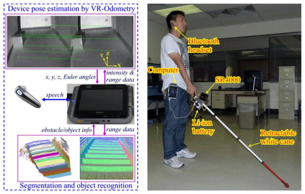
To perform autonomous navigation, a mobile robot must perceive its surrounding in 3-D and understand the scene by processing the 3-D range data. 3-D LIDAR [1], [2], and stereovision [3] have been widely used in the existing research. However, a 3-D LIDAR is not suitable for a small-sized robot because of its dimension and weight, while a stereovision system may not produce reliable 3-D data for navigation due to the need of dense feature points for stereo-matching. Also, a stereovision has another disadvantage: its range measurement error increases quadratically with the true distance. Alternatively, a depth camera, such as Microsoft Kinect sensor [4] or flash LIDAR camera (FLC) [5], may be used to navigate a small robot. The Kinect is a cost-effective RGB-D camera for robotic application and has been recently used in indoor robotic mapping and navigation [6]–[8]. However, the sensor determines depth based on triangulation. As a result, its range accuracy drops with the true distance, just like a stereovision system. We are developing a robotic navigation aid, called smart cane (SC) [9], for guiding a visually impaired person in an indoor environment. To satisfy the portability and accuracy requirement, a FLC (SwissRanger SR4000), instead of a Kinect sensor, is used in the SC for 3-D perception. Our SC prototype is depicted in Fig. 1. It has two navigational functions: 6 degrees of freedom pose estimation and object detection/recognition. For pose estimation, the computer (worn by the SC’s user) simultaneously processes the FLC’s intensity and range data and determines the SC’s pose change between each two image frames [10]. This pose change information is then used to compute the device’s pose in the world coordinate for way-finding and registering range data (captured at different locations along the path) into a 3-D point-cloud map of the environment. For object detection/recognition, the 3-D point-cloud data is first segmented into planar surfaces, which are then clustered into objects for object detection. Eventually, the detected objects are used for obstacle avoidance or used as waypoints for navigation. For instance, an overhanging object will trigger an obstacle warning and/or evoke an obstacle avoidance action; while a stairway may be used as a way-point to access the next floor, and a doorway a waypoint to get into/out of a room. The SC’s capability in detecting and using these waypoints may help a blind traveler move around more effectively in an indoor environment. Due to the limited computing power of the SC, a fast plane extraction (PE) method is required.
Fig. 1.
Smart cane: a computer-vision-enhanced white cane.
II. Related Work on Plane Extraction
Plane extraction methods in the literature may be broadly classified into two categories: edge-based and region-growing algorithms. An edge-based approach [11], [12] detects the edges of a range image and uses them to bound the planar patches. It assumes that edges are the borders between different planar surfaces that have to be segmented separately. A region-growing algorithm [13]–[17] selects some seed points in range data and grows them into regions based on the homogeneity of local features (see surface normal, point-to-plane distance, etc.). Xiao et al. proposed a cached-octree region-growing (CORG) algorithm [14] for extracting planar segments from a 3-D point set. The k nearest-neighbor (k-NN) search routine is used for constructing the cached-octree and retrieving the k-NN of a point. The algorithm starts from a region G, consisting of a point and its neighbors, with the minimum plane-fitting error. The algorithm then grows G by adding its neighboring point pc to G if both the distance between pc and the least-square plane of G ∪ pc and the plane-fitting error are sufficiently small. This region-growing process continues until no more points may be added to G. Once a planar segment is extracted, the algorithm removes the extracted data points from the 3-D point set and starts a new PE procedure. Since the method stops region-growing merely based on distance information, over-extraction may occur at the intersection of two planes. The invariants of this point-based region-growing method are the grid-based [16] and super-pixel-(SP-)based [17] algorithms. The grid-based region-growing algorithm [16] divides a range image into a number of small grids whose attributes are computed and used for region growth. The SP-based approach clusters the range image of a 3-D point set into numerous homogeneous regions (called SPs) based on the local features of the image pixels and partitions the SPs into a number of planar segments using the similarities between the SPs. An experimental comparison of some earlier range image segmentation methods is presented in [18] where the algorithms’ parameters were manually tuned. A similar performance evaluation study is performed in [19] with automated tuning of parameters. A region-growing method is sensitive to range data noise. For instance, the SR4000’s range data noise may significantly affect the surface normals of the data points and thus the segmentation result. The co-author of this paper demonstrates that using a graph-cut method (the normalized cuts) to partition the SPs (homogeneous range image regions clustered by the mean-shift method) into planar segments may mitigate the effect of range data noise [20]. As demonstrated in [18] and later in [22], the segmentation problem is still open even for a simple scene with polyhedral objects. The reason is that it is difficult to correctly identify small surfaces and preserve edge locations.
Hybrid approaches [21]–[24] combining the use of edge-based and region-growing methods have also been attempted to improve the reliability and accuracy of range image segmentation. This type of methods may incur a much higher computational cost since both edge-based and region-growing methods are used. Nurunnabi et al. [23], [24], divided plane segmentation into three steps: classification, region growing, and region merging. Their method uses the robust principal components analysis (RPCA) method to classify 3-D points into edge-points, boundary-points, and surfels. It then grows a region by adding a neighboring surfel point if the seed-surfel-normal-angle (i.e., the angle between the normal of the region’s seed point and that of the surfel point) is below a threshold. The edge-/boundary-points found by the RPCA are used to identify region boarders (i.e., to stop a region-growing process). The RPCA-based method works well for a scene with distinct edges between intersecting planes (i.e., with small plane angles). However, it may fail if the edges are indistinct. This will be explained with experimental results in Section VII.
A model-based method may be viewed as a region-growing approach since it clusters data points with similar property (i.e., fit to the model) into a plane. A model-based segmentation method works well for a scene where objects can be described by mathematical models, e.g., plane, sphere, curved surface, etc. Hough transform (HT) plane detection [25] is a typical model-based method where each data point cast its vote in the HT parameter space and the accumulator cells (the HT parameters) with the largest number of votes are identified as the parameters for the model. The issues of the HT method are the high computational cost in fitting a mathematical model to a large data set and the sensitivity to accumulator design. The robust moving least-squares fitting method proposed by Fleishman et al. [26] may be used for plane segmentation. The method employs a robust estimator to identify the least median of squares (LMS) plane of a number of points by fitting a plane to the points and computing the median of the residuals of the fit. Differing from [14], it grows this LMS point set using a forward search algorithm (FSA). The FSA adds to the point set i points (out of all neighboring points of the set) with smallest residuals, meaning that the threshold value for region-growing is dynamically determined. The method shares the common features of the CORG [14] in that it uses point-to-plane distance as a sole criterion for region-growing. As a result, it may also incur over-extraction. Random sample consensus (RANSAC) [27] has been widely used in model-based methods for PE. A typical RANSAC PE method [28] is a repeated process of fitting a hypothesized plane to a set of 3-D data points and accepting points as inliers if their distances to the plane are below a threshold. The process attempts to maximize the total number of inliers. The disadvantage of the standard RANSAC PE method is that it may fail when a scene contains multiple intersecting planar surfaces with limited sizes [29]. In this case, the method extracts a plane straddling over multiple planar surfaces because such a plane contains the largest number of inliers. These inliers consist of a number of separate inlier patches, each of which is part of the corresponding planar surface. This phenomenon will be further explained in Section IV. To overcome this problem, Gallo and Manduchi [29] proposed the CC-RANSAC method. The idea is to check the inliers’ connectivity, select the largest inlier patch, and grow the patch into a plane in its entirety. The CC-RANSAC method solves the straddling-plane problem when the scene contains simple steps/curbs. However, it may fail when the scene is complicated so that the inlier patches resulted from the RANSAC plane-fitting process are connected (i.e., inseparable). This scenario will be explained in Section IV. To overcome the limitation of the CC-RANSAC method, we propose a normal-coherence CC-RANSAC (NCC-RANSAC) method for PE in this paper. The NCC-RANSAC method checks the normal coherences for all data points of the inlier patches (on the fitted plane) and removes the data points whose normal directions are contradictory to that of the fitted plane. This process results in a number of separate inlier patches, each of which is treated as a seed plane. A recursive plane clustering process is then executed to grow each of the seed planes until all planes are extracted in their entireties. The RANSAC plane-fitting and the recursive plane clustering processes are repeated until no more planes are found.
This paper is organized as follows: Section III gives a brief description of the SwissRanger SR4000. Section IV details the disadvantages of the RANSAC and CC-RANSAC PE methods. Section V presents the NCC-RANSAC method. Section VI compares the computational costs of the CC-RANSAC and NCC-RANSAC and introduces a model for predicting the success probability of the NCC-RANSAC and some metrics for quality evaluation of extracted planes. Section VII presents experimental results with real sensor data and comparison with the related methods. The paper is concluded in Section VIII.
III. SwissRanger SR4000
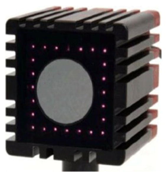
The SwissRanger SR4000 [5] (Fig. 2) is a time-of-flight (TOF) 3-D camera. The TOF is determined by phase shift measurement. The camera illuminates its environment by amplitude modulated infrared light (850 nm). Its CMOS imaging sensor measures the phase shift of the returned modulated signal at each pixel. The amplitude and phase shift of the signal are used to determine the intensity and distance of the target point. As a result, the camera delivers both intensity and range images for each captured frame. The camera has a spatial resolution of 176 × 144 pixels and a field of view of 43.6° × 34.6°. Its nonambiguity range is 5 m when a modulation frequency of 30 MHz is used. The programmable modulation frequency (29/30/31 MHz) allows simultaneous measurements of three cameras without interference. The camera has a small physical dimension: 65 × 65 × 68 mm3. This makes it an ideal sensor for the SC. However, as a TOF camera the SR4000 incurs a larger range measurement noise compared to a LIDAR. This requires a PE method that is robust to range data noise. Some of the SR4000’s key specifications are tabulated in Table I.
Fig. 2.
SwissRanger SR4000.
TABLE I.
Specification of the SR4000 (Model: SR 00400001)
| Non-ambiguity range | 5 m |
| Absolute accuracy | ±10 mm (typ.) |
| Repeatability (1 σ) | 4 mm (typ.), 7 mm (max.) |
| Pixel array size | 176 (h) × 144 (v) |
| Field of view | 43.6° (h) × 34.6° (v) |
| Modulation frequency | 29/30/31 MHz |
| Acquisition mode | Continuous/ triggered |
| Integration time | 0.3 to 25.8 ms |
| Dimension | 65 × 65 × 68 mm |
| Weight | 470 |
typ.: typical, max.: maximum, h: horizontal, v: vertical
IV. Limitations of RANSAC and CC-RANSAC
A RANSAC plane-fitting method may produce incorrect result when the data contains small steps (e.g., curbs, stairways, etc.). Fig. 3 shows a 2-D (cross section) view of the RANSAC plane-fitting on a stairway scene. For an M-step stairway, the scene contains N = 2M planes. Without losing generality, we assume that the scene has an identical point density and the side length of each plane is measured in term of number of data points. The total length of a step (i.e., AB + BC) in the cross section is 2L/N, where L is the total length of the stairway. The RANSAC algorithm may result in a slant plane (depicted by the oblique solid line in Fig. 3) straddling multiple steps because this plane produces more data points satisfying di < δ than any plane on a stair riser (AB) or a stair tread (BC). In Fig. 3, the data points of the stairway between the two planes (depicted by the dotted lines) satisfy di < δ and their number is , where W is the stairway’s width. The number of data points of AB or BC, whichever is larger, is . The RANSAC method results in a slant plane (with slope ) straddling all steps if , i.e.,
Fig. 3.
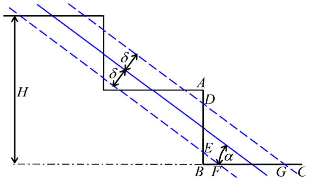
RANSAC plane-fitting on a stairway scene: h—stairway height, AB—height of stair riser, BC—depth of stair tread, δ—distance threshold for plane-fitting. Each of them is measured in term of number of data points. α—stairway slope.
| (1) |
For a case with L = 144 pixels, δ = 1, and α = 30°, we obtain N > 7.6 from (1). This means that the RANSAC PE method fails if the number of planes of the stairway is greater or equal to 8. In this case, it results in a slant plane instead of 8 stairway planes (riser and tread planes).
When a stairway contains only horizontal planes (treads), (1) may be simplified to
| (2) |
With the same parameters of the above case, we get N > 6, meaning that the RANSAC method fails if the number of planes of the stairway is greater than 6.
It can be observed that a plane straddling multiple planes produces multiple disconnected planar patches. The CC-RANSAC method seeks to maximize the number of connected inliers. Without losing generality we assume AB < BC (i.e., DE < FG) in Fig. 3. The CC-RANSAC selects the largest contiguous inlier set (i.e., FG), attempts to maximize its data points, and eventually obtains plane BC. The CC-RANSAC process continues on the remaining data until no more planes are found.
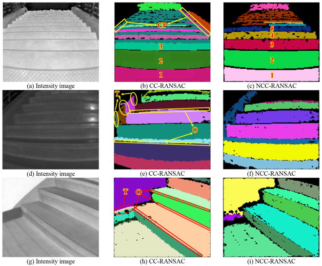
The CC-RANSAC method has two limitations though. First, It may over-extract a plane, i.e., it does not extract the exact planar patch for the inliers when there are intersecting planes. Fig. 4(a) depicts a scene with a horizontal plane connected with a vertical plane. The CC-RANSAC method results in the plane depicted by the dotted lines. The inliers include all data points on the horizontal plane and the data points on the lower portion of the vertical plane because all of these data points satisfy di < δ. This over-extraction looks like that the horizontal plane swallows part of the vertical plane. Second, the CC-RANSAC method may fail in case of a scene with a stairway that contains a stair wall. This is illustrated in Fig. 4(b) where the fitted plane (ABC) results in a number of inlier patches (p2, p3, …, p6) on the stairway’s risers and treads and an inlier patch (p1) on the stairwall. As p1 connects all the other patches to form a single contiguous inlier set, the CC-RANSAC is unable to find any inlier patch that is on a riser or a tread. It is noted that the CC-RANSAC method may perform well if the step number of the stairway is small such that a horizontal/vertical plane fitted to a tread/riser produces more inlier data points than a slant one. However, in this case the inliers on the stair wall become horizontal/vertical and they are part of the extracted tread/riser plane. These inliers look like a tail to the extracted plane. The tail phenomenon is another embodiment of the CC-RANSAC’s over-extraction limitation. [This problem will be demonstrated later in Section VII in Fig. 11(e) and (h)].
Fig. 4.
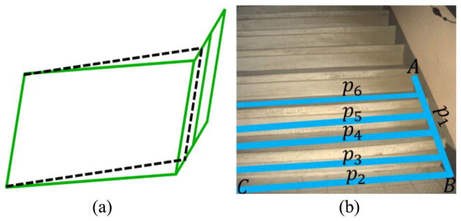
CC-RANSAC plane-fitting in case of intersecting planes or a stairway with a stair wall. (a) Intersecting planes. (b) Stairway with a stair wall.
Fig. 11.
Experimental results with real data (single frame): the NCC-RANSAC results are before filling the missing points. (a) Intensity image. (b) CC-RANSAC. (c) NCC-RANSAC. (d) Intensity image. (e) CC-RANSAC. (f) NCC-RANSAC. (g) Intensity image. (h) CC-RANSAC. (i) NCC-RANSAC.
V. NCC-RANSAC Plane Extraction
The idea of the NCC-RANSAC method is two-fold. First, it examines the normal coherence of all inliers resulted from the RANSAC plane-fitting. The normal coherence test exploits the fact that the stair wall’s normal is perpendicular to that of the fitted plane (ABC). An inlier data point satisfying β= 90° is thus removed because it violates normal coherence. Here, β is the angle between the surface normal of the inlier and the fitted plane. This process removes the small patch on the stair wall [p1 in Fig. 4(b)] and results in a number of disconnected planar patches (p2, p3, …, p6) on the risers/treads. Second, instead of looking for the largest patch, the NCC-RANSAC treats each of the resulted patches as a candidate plane and performs an iterative plane clustering process as follows: 1) a plane is fitted to the patch and the distance from each data of the scene to the plane is calculated; 2) data point with a sufficiently small distance is added to the patch; and 3) steps 1 and 2 repeat until no data may be added to the patch. It is noted that the actual angle between the normals of the stair wall and the fitted plane for the SR4000’s data is not 90° due to range data noise. In this paper, we use |β−90°|< 40° for normal coherence test.
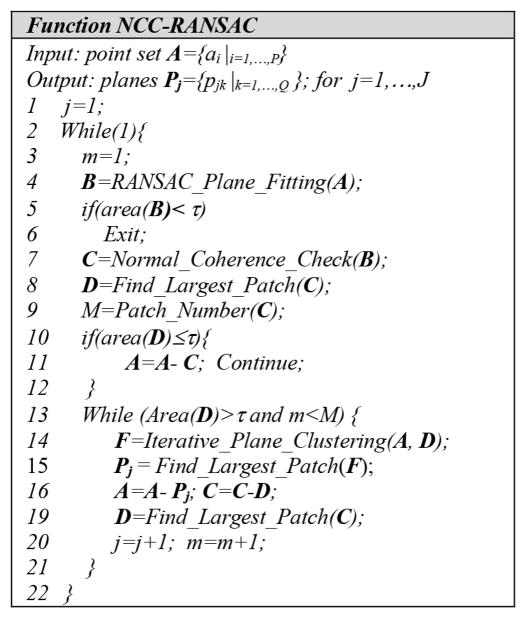
The pseudo code of the NCC-RANSAC is illustrated in Fig. 5. In line 4, A RANSAC plane-fitting process is applied to the input point set to identify a plane with the maximum number of inliers. The inliers are then checked for normal coherence in line 7 to produce a set of isolated inlier patches. The number of inlier patches M is determined in line 9. The inner while loop (lines 13–21) is an iterative plane clustering procedure that finds the plane for each significant inlier patch (i.e., a patch with an area larger than τ). In this process, a plane is fitted to the inlier patch. A point satisfying the following two criteria is assigned to the plane and thus grow the plane: 1) the point-to-plane distance is smaller than a threshold δ and 2) the angle between the point’s surface normal and the plane’s normal is smaller than a threshold θ0. Once a plane is extracted, its data points and the data points of the inlier patch are subtracted from the point set and the set of inlier patches, respectively (line 16). The updated set of inlier patches are then used for the plane clustering procedure. The while loop repeats until all of the significant inlier patches are exhausted. The entire NCC-RANSAC loop (the outer while loop) is repeated until no significant patch is found by the RANSAC plane-fitting. It can be observed that the NCC-RANSAC method uses one RANSAC plane-fitting procedure to find multiple inlier patches, each of which is then used as a seed to grow and extract the corresponding plane. As a result, the NCC-RANASC method is much more computationally efficient than the CC-RANSAC method.
Fig. 5.
Pseudocode of the NCR-RANSAC algorithm: τ is threshold value.
VI. Performance of NCC-RANSAC
A. Computational Cost
In this section, we give an analytical comparison on the computational costs of the two methods–CC-RANSAC and NCC-RANSAC. To simplify the analysis, we use a stairway case as shown in Fig. 3 and assume: 1) the risers and treads have the same size and 2) the two methods’ plane-fitting calculations in each step have the same computational time. For the CC-RANSAC method, it requires a RANSAC plane-fitting process to extract each plane. The true inlier ratio for extracting the ith plane is 1/(N + i−1) for i = 1, …, N. The minimum number of iteration for extracting the plane with a confidence level η that the plane is outlier-free is given by
| (3) |
where n is the number of data points that are used to generate the hypothesized plane. In this paper, n = 3. Therefore, the total number of RANSAC plane-fitting processes required by the CC-RANSAC is
| (4) |
where N is the number of planes of the stairway.
Following the similar analysis, the required number of RANSAC plane-fitting processes for the NCC-RANSAC method is determined by:
| (5) |
where . Equation (5) indicates that if inequality (1) is met (i.e., the slant plane occurs) the computational cost of the NCC-RANSAC includes the cost of a RANSAC plane-fitting procedure (line 4 in Fig. 5) and the cost of the rest of the method (lines 5–21) which can be approximated by the computational cost of the while loop (lines 13–21) (i.e., C1N). Otherwise, the NCC-RANSAC becomes CC-RANSAC plus normal coherence check and therefore its computational cost contains two portions: the cost of the CC-RANSAC (i.e., KCC (N)) and the cost of lines 5–12 that may be approximated by the cost of line 7 (i.e., C2N). It is noted that terms C1N and C2N are measured as the equivalent number of RANSAC plane-fitting processes. C1 and C2 are constant numbers and their values are experimentally determined as C1 = 120 and C2 = 30.
For the simplified case with only horizontal planes (i.e., treads). Equation (5) becomes
| (6) |
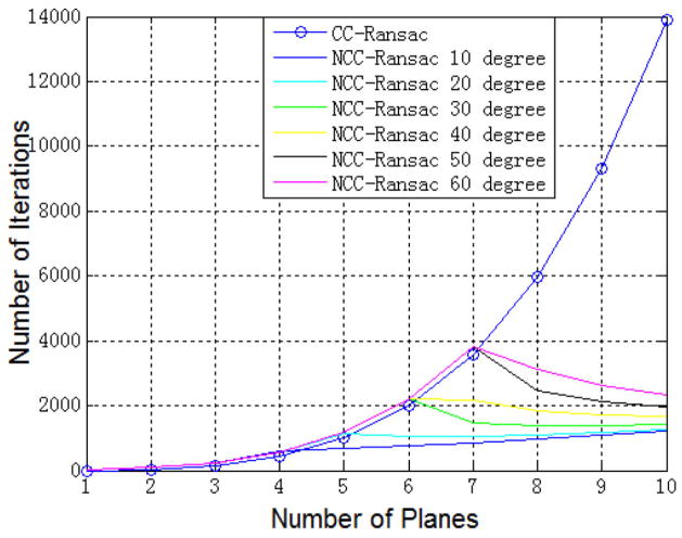
where . Fig. 6 depicts the plot of K versus N with conditions L = 144 and δ = 1. Generally, KCC(N) grows quickly with N and KNCC(N, α) follows the similar curve of KCC(N) before the turn point (at ) meaning that it has the similar computational cost as the CC-RANSAC. However, KNCC(N, α) stops growing after the turn point. It first drops down and then grows very slowly with increasing N. In theory, the NCC-RANSAC method has a much lower computational cost than the CC-RANSAC if the fitted plane straddles across multiple planes of the stairway.
Fig. 6.
Comparison of computational cost for stairway scenes with varying slope (α = 10° ~ 60°).
B. Quality of Extracted Planes
The quality of an extracted plane is evaluated by the plane-fitting error. For an extracted plane containing M data points, the plane-fitting error is given by
| (7) |
where di is the distance from the ith data point to the plane. When the ground truth data is available, two additional metrics, et and ξn, may be used to evaluate how well the extracted plane represents the ground truth plane. Here, et is calculated by (7) using the distances from the ground truth data points to the extracted plane, and ξn is the angle between the normals of the extracted plane and ground truth plane. We will use these metrics to evaluate the NCC-RANSAC method’s performance in Section VII.
C. Robustness to Range Data Noise
The use of the normal criterion for the iterative plane clustering process leads to improved plane smoothness. However, it makes the method sensitive to range data noise. In this paper, we propose a probabilistic model to evaluate the method’s robustness to range data noise. The model calculates the likelihood of successfully extracting a plane by the NCC-RANSAC method.
We assume that the x, y, and z coordinates of each range data point have a white Gaussian noise N(0, σ2), i.e., the probability density function of the noise is , where * stands for x, y, or z noise. To determine the surface normal for a noise-corrupted point q(i, j) in the range data, we fit a paraboloid to the 3 × 3-point patch Ω(i, j) = {q(k, l) |k=i−1,i,i+1; l=j−1,j,j+1}surrounding q(i, j). In this patch, q(i, j)’s neighboring points are ground truth data. To simplify the denotation, we consider a scene with only one plane that is perpendicular to the SR4000’s optical axis. Fig. 7 depicts a 2-D view of the paraboloid fitting on a 3 × 3-point patch Ω(iy, jx), of which point q(iy, jx) (denoted by Q) is the data of the SR4000’s central imaging pixel. In Fig. 7, O represents the ground truth of q(iy, jx), while B and A denote points q(iy, jx − 1) and q(iy, jx + 1), respectively.
Fig. 7.
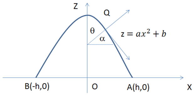
2-D chart (XZ plane) for paraboloid fitting.
According to the SR4000’s specifications, we have , where v = 40 μm, f = 10 mm and do are the camera’s pixel pitch, focal length and the range value of point p(iy, jx), respectively. θ is the angle between the surface normal at Q and the normal of ground truth plane (i.e., normal of noise-free point O). For a plane with do = 3 m, we have h = 12.6 mm. If θ ≤ θ0, point Q meets the angular criterion and is thus classified as a point in the ground truth plane. From Fig. 7, we can derive
| (8) |
where x is point Qs x coordinate. As we actually fit paraboloid z = a (x2 + y2) + b to the data point, (8) should become
| (9) |
The angular criteria θ ≤ θ0 is met if point Q satisfies , where |x| ≤ h and |y| ≤ h. Q can be in any of the eight octants in the 3-D coordinate. Therefore, the probability that point Q is part of the ground truth plane is given by
| (10) |
where . It is noted that the use of the above-mentioned special conditions does not cause loss of generality to (10). For a general case where the plane is not perpendicular to the camera’s optical axis and/or Q is the data point of an off-the-center pixel, we can prove BO ≈ AO > h. A larger h will reduce θ. Therefore, θ < θ0 is still met. We omit the proof for conciseness.
Assuming that the NCC-RANSAC algorithm is regarded as successful if it extracts 60% of a scene’s data points, the probability of success can be computed by
| (11) |
where n is the number of data points of the scene.
VII. Simulation and Experimental Results
A. Computational Cost
To validate the computational cost model, we generated synthetic stairway data by computer simulation and ran the NCC-RANSAC and CC-RANSAC algorithms on the data. Two of the simulation results are shown in Fig. 8. Fig. 8(a) and (b) shows a stairway case with α = 10° and α = 40°, respectively. The turn points (N = 4 and N = 6) and the computational times before and after the points agree with the theoretical values as plotted in Fig. 6.
Fig. 8.
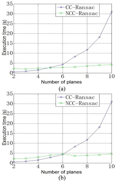
Real execution time for a stairway with various slopes. (a) α = 10°. (b) α = 40°.
B. Quality of Extracted Planes
Due to the difficulty in obtaining ground truth scene, we built a SR4000 simulator to generate synthetic range data. The simulator first produces a point cloud with even density for a scene. A Gaussian noise N(0, σ2), where σ = ρd, is added to each data point. Here, ρ is the SR4000’s noise ratio and d is the true distance. According to the SR4000’s specification [5], ρ < 0.2%. Therefore, we used ρ = 0.2 in this paper. The simulator then performs a perspective projection using the SR4000’s imaging model to generate range data points.
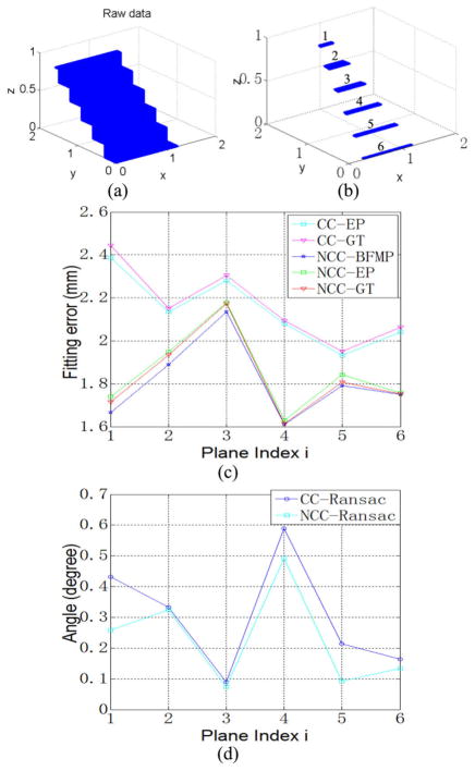
In case study 1, the synthetic data [Fig. 9(b)] is generated from a raw stairway point cloud [Fig. 9(a)] with the SR4000 locating at [0.75, 1.9, 1.37 m] and pointing toward [0, −1, −1]. The plane-fitting errors, et and ea, and the angular errors of plane normal ξn of the NCC-RANSAC and CC-RANSAC methods are shown in Fig. 9(c) and (d), respectively. It can be seen that the extracted planes of the NCC-RANSAC method have smaller plane-fitting errors (both et and ea) and smaller ξn. It is noted that after the NCC-RANSAC we actually smoothed the plane by filling in the missing points that are encompassed by the plane and meet the distance criteria. As can be seen from Fig. 9(c), adding these missing points only slightly increases the plane-fitting error.
Fig. 9.
Plane-fitting errors and angular errors of plane normal of NCC-RANSAC and CC-RANSAC. CC: CC-RANSAC. NCC: NCC-RANSAC. EP: extracted plane. GT: compare with ground truth. BFMP: before finding missing points. (a) Point cloud with even density. (b) Synthetic SR4000 range data. (c) Plane fitting error (ea/et). (d) Error of plane normal (ξn).
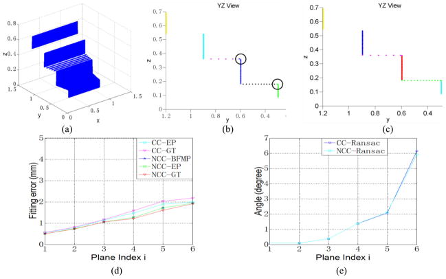
In case study 2, the same point cloud is used and the camera is pointed toward [0, 1, −0.1] from position [0.625, −1.5, 0.55 m] to generated synthetic range data [Fig. 10(a)]. The PE results are shown in Fig. 10(d) and (e). Again, the NCC-RANSAC method results in smaller et, ea, and ξn. Fig. 10(b) and (c) show the Y-Z view of the extracted planes by the two methods. It can be observed that the CC-RANSAC method causes the two riser planes (vertical planes) to swallow part of the tread planes (horizontal planes) of the steps as circled in Fig. 10(b). This problem is resolved in the NCC-RANSAC method [Fig. 10(c)].
Fig. 10.
Plane-fitting errors and angular errors of plane normal of NCC-RANSAC and CC-RANSAC. (a) Synthetic SR4000 data. (b) CC-RANSAC. (c) NCC-RANSAC. (d) Plane fitting error (ea/et). (e) Error of plane normal (ξn).
The NCC-RANSAC outperforms the CC-RANSAC due to the fact that the normal coherence check and the use of normal in the plane clustering process allow the NCC-RANSAC to extract the exact plane while the CC-RANAC may over-extract the plane (i.e., swallow part of its neighboring plane).
We have also carried out experiments with real sensor data captured in various indoor environments. Fig. 11 depicts the results from three of the experiment. The NCC-RANSAC produces better results than the CC-RANSAC. For the 1st experiment, the NCC-RANSAC successfully extracts the five prominent planes while the CC-RANSAC fails in extracting the 4th and 5th planes because the coplanar (inlier) patches on the stair walls [labeled as CP in Fig. 11(b)] connects the inlier patches on the stairway’s steps and forms a plane with the largest number of data points. For the 2nd experiment, we can observe noticeable over-extraction in the result of the CC-RANSAC [Fig. 11(e)]. There are tails (labeled as T) in several of the extracted riser planes. Also, several of the extracted riser planes swallow part of their neighboring tread planes and result in narrower extracted tread planes. These over-extractions are labeled as O in Fig. 11(e). However, the NCC-RANSAC extracts each plane exactly [Fig. 11(f)]. Similar over-extraction problems occur in the tread plane in the 3rd experiment [Fig. 11(h)] but the NCC-RANSAC obtains each plane exactly.
C. Robustness to Range Data Noise
Using (10) we compute Pu with different combinations of ρ and θ0 for a scene with a single plane. The results are tabulated in Table II. Assuming that the scene has n data points, we calculate P(n) for each Pu by (11). The results are plotted against n in Fig. 12. We can see that the NCC-RANSAC has over 70% probability of success for ρ = 0.2% and the value of P(n) increases with increasing n and θ0. When θ0 ≥ 50°, P(n) rapidly approaches to 100% with increasing n. In theory, the method breakdowns (extracts less than 60% points for a plane) at ρb = 0.24% if θ0 = 45°. The value of ρb may be slightly larger if loose criteria (larger θ0 and lower percentage of extracted points) are used.
TABLE II.
Pu With Different Angular Conditions and Noise Ratios
| θ0 | 45° | 50° | 55° | 60° |
|---|---|---|---|---|
| ρ | ||||
| 0.1% | 0.9444 | 0.9460 | 0.9476 | 0.9488 |
| 0.2% | 0.6380 | 0.6616 | 0.6828 | 0.7008 |
| 0.3% | 0.3416 | 0.3660 | 0.3892 | 0.4124 |
| 0.4% | 0.1892 | 0.2064 | 0.2240 | 0.2424 |
Fig. 12.
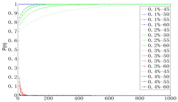
P(n) versus n with different combinations of ρ–θ0 pairs.
To validate the probabilistic model, we captured a number of data sets from the SR4000 with various indoor scenes. Fig. 13 depicts a typical indoor scene that we used for the experiment. For each scene we acquired 1000 frames. We determined n of each plane in a scene by labeling the plane in the intensity image and counting its pixel number. We then calculated the range data noise ratio for each pixel using its mean and standard deviation over the 1000 range data samples. The overall noise ratio ρ̂ for the plane’s range data is estimated as the mean noise ratio of all of its data points. The experimental probability of success Pe(n) of the method for each plane is determined as the success rate of the PE of the 1000 frames. In our experiment, we used θ0 = 45°. The noise ratios of the SR4000’s range data are mostly around 0.1% when the sensor is in auto-exposure mode. To generate range data with larger ρ, we set the sensor to manual exposure mode and used a smaller exposure time. Table III shows the results from two typical experiments. We can see that a larger n and/or a smaller ρ̂ result in a larger Pe(n). This means that the actual probability of success agrees with the theoretical value given by (11). Equation (11) provides us a way to predict the NCC-RANSAC’s probability of success in extracting a particular plane.
Fig. 13.
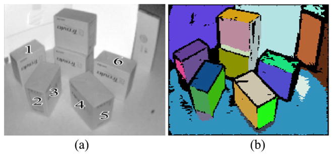
NCC-RANSAC with SR4000 data (single frame): scene 1. (a) Intensity image. (b) Extracted planes.
TABLE III.
Success Rate of Plane Extraction
| Scene I | Scene II | ||||||
|---|---|---|---|---|---|---|---|
| PI | PN | ρ̂ | Pe(n) | PI | PN | ρ̂ | Pe(n) |
| 1 | 397 | 0.175 | 0.933 | 1 | 477 | 0.202 | 0.917 |
| 2 | 463 | 0.211 | 0.912 | 2 | 449 | 0.214 | 0.902 |
| 3 | 511 | 0.235 | 0.902 | 3 | 404 | 0.189 | 0.926 |
| 4 | 508 | 0.227 | 0.883 | 4 | 359 | 0.190 | 0.909 |
| 5 | 560 | 0.202 | 0.957 | 5 | 477 | 0.205 | 0.911 |
| 6 | 550 | 0.241 | 0.926 | 6 | 729 | 0.212 | 0.979 |
PI–Plane Index, PN–Point Number
Our experiments with smaller ρ̂ and/or larger θ0 in various indoor environments indicate that the values of Pe(n) are very close to 1. Since ρ̂ of the range data of the SR4000 are around 0.1% in many cases, we may claim that the NCC-RANSAC has a rate of success very close to 100%.
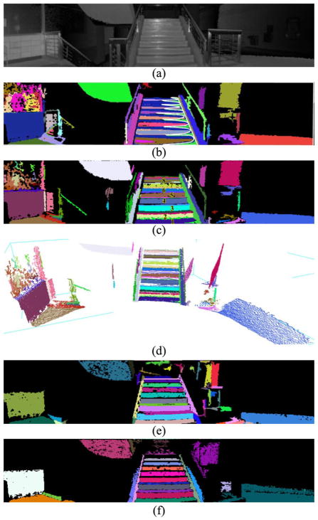
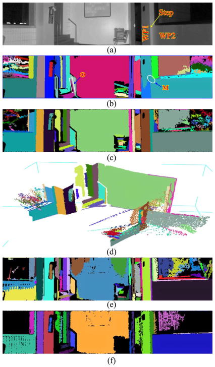
Experimental results with larger views are shown in Figs. 14 and 15. Each scene is formed by registering 9 intensity/range images that were captured consecutively from the SR4000 with a 15° pan movement. The horizontal view angle of each scene is therefore 120°. We applied both the NCC-RANSAC and CC-RANSAC to these range data and the results are depicted in Figs. 14 and 15. For the 1st experiment (Fig. 14), the NCC-RANSAC [Fig. 14(c)] successfully exacts the eight risers (vertical planes of the stairway) as well as the wall plane and floor plane. However, the CC-RANSAC produces two slant planes. One is labeled in green and enclosed with the white lines. The other one is labeled in blue (on the stairway planes). Each slant plane consists of a number of small patches (blue/green) belonging to the stairway planes. For the 2nd experiment (Fig. 15), the CC-RANSAC method over-extracts one of the steps of the stairway [labeled by the white rectangle in Fig. 15(b)]. Also, there are misclassified planes on the wall (in the right of the image). The two wall planes (WP1 and WP2) with a small step in Fig. 15(a) are misclassified as one plane [Fig. 15(b)]. The white ellipse [in Fig. 15(b)] shows the area where the two wall planes and the step plane join. However, the NCC-RANSAC method successfully extracts all three planar surfaces [Fig. 15(c)]. The point clouds of the extracted planes, labeled in different colors, for the two experiments are shown in Figs. 14(d) and 15(d), respectively.
Fig. 14.
Experimental results with real data (stitched range data): scene 2. (a) Intensity image. (b) CC-RANSAC. (c) NCC-RANSAC. (d) NCC-RANSAC: 3-D view (point cloud) of the extracted planes. (e) CORG. (f) RPCA.
Fig. 15.
Experimental results with real data (stitched range data): scene 3. (a) Intensity image. (b) CC-RANSAC. O: Over-extraction. M: Misclassification. (c) NCC-RANSAC. (d) NCC-RANSAC: 3-D view (point cloud) of the extracted planes. (e) CORG. (f) RPCA.
D. Comparison With Other Methods
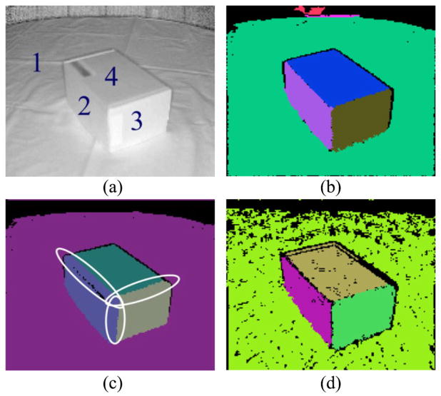
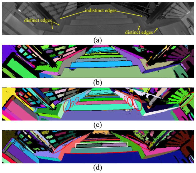
We implemented the CORG method [14] and the RPCA-based hybrid method [23] and the results are compared with those of the NCC-RANSAC in Figs. 16 and 17. Fig. 16(a) is the intensity image of a scene with a cardboard box, where the four planes are marked. The NCC-RANSAC method and RPCA-based method extract all four planes. However, the CORG method results in over-extractions at the intersections between planes 2, 3, and 4 [marked by the white ellipses in Fig. 16(c)]. It is noted that the planes extracted by the NCC-RANSAC are free of missing points as its plane smoothing process filled up the missing data. Fig. 17 shows the results on a stairway scene. Similar to Fig. 14, the data is generated by stitching 9 intensity/range images. Again, the NCC-RANSAC method successfully extracted the treads and stairwalls in their entireties. The CORG method incurs over-extractions [marked by the red ellipses in Fig. 17(c)]. The RPCA-based method successfully extracts planes for the portion of scene with distinct edges [Fig. 17(d)]. However, it failed at indistinct edges (marked by the red ellipses). Also, the method results in under-extraction (marked by the white rectangle). The results of the CORG and RPCA methods for scenes 2 and 3 are also shown in Figs. 14 and 15, respectively, from which we can observe that the NCC-RANSAC achieves better segmentation results.
Fig. 16.
Segmentation results of the methods with SR4000 data (single frame): scene 4. (a) Intensity Image. (b) NCC-RANSAC. (c) CORG. (d) RPCA hybrid.
Fig. 17.
Segmentation results of the three methods with SR4000 data (stitched range data): scene 5. The over-extractions (tails) of the CORG may have negative impact on pattern recognition if the shortest distance between the points in two planar segments is used to describe the intersegment relationship. The RPCA-based method failed at the indistinct edges. (a) Intensity image. (b) NCC-RANSAC. (c) CORG. (d) RPCA hybrid.
It is noted that the RPCA-based method is sensitive to the angular threshold used for region-growing. A larger value results in greater over-extractions, while a smaller one leads to heavier under-extractions. In our case, the noise of the SR4000 tends to cause heavy under-extractions. To overcome this problem, a larger threshold should be used. However, this may cause over-extraction at an indistinct edge because the seed-surfel-normal-angles are smaller than the threshold. Fig. 17(d) depicts the segmentation result with the best threshold value (35°) we found for the scene. It can be seen that both under-extraction and over-extraction occur. (As demonstrated in our experiment, a 5° threshold as used in [23] resulted in excessive under-extractions that break each plane into many segments.) Similarly, the CORG method should use larger thresholds (distance values) for region-growing in order to reduce noise-induced under-extractions. However, this may result in larger over-extractions at the edges [Fig. 16(c)] and larger tails on intersecting planes [Fig. 17(c)]. In principle, the tail over-extraction cannot be eliminated. Taking Fig. 17(c) as an example, the tail is reduced into a line (but cannot be removed) if the thresholds are set to zero. Because the data points on each tail are coplanar with the extracted plane and thus meet the region-growing criteria. The NCC-RANSAC overcomes the disadvantages of the two methods by using both distance and angular criteria for region-growing.
The runtimes of the three methods for the scenes of Figs. 13–17 are tabulated in Table IV. The NCC_RANSAC method is slower than the RPCA for scenes 2, 3, and 5 because it performed plane-fitting for each data point in region-growing and each of the scenes contain a large number of planes. However, the NCC-RANSAC is faster for the scenes with a lower number of planes (scenes 1 and 4). With respect to the runtimes of the other two methods (NCC-RANSAC and CORG), the NCC-RANSAC outperforms the CORG in all cases. In particular, the NCC-RANSAC took much less time than the CORG for a scene with large planar surfaces (i.e., small number of planes). This is because the RANSAC model fitting approach is much more computationally efficient than the region-growing method. This feature makes the NCC-RANSAC well-suited to the SC because the dominant scenes in an indoor environment are large planar surfaces such as the ground and/or walls.
TABLE IV.
Execution Time for PPDB and NCC-RANSAC
All methods were implemented in MATLAB R2012b on a desktop with an Intel i7-2600K CPU, 8 GB memory, and Windows 7 as OS. The runtime of the NCC-RANSAC may be drastically reduced if it is implemented in C code. Also, it is noted that the method introduced in [15] for incremental computation of least-squares plane may be employed by the proposed method for plane clustering and further save the computational time. Finally, the NCC-RANSAC is ideal for GPU implementation since both the RANSAC plane-fitting process and the plane clustering process are independent ones. The GPU implementation in the future may achieve a high order of speed-up for real-time operation. It is noted that a runtime of 1 s may be considered as real-time operation for the SC application. The proposed method is promising in achieving this goal.
In the experiments, we used threshold values δ = 10 mm and θ0 = 45° for plane clustering. δ was determined as the SR4000’s absolute accuracy (±10 mm (5)]. θ0 was computed from the paraboloid function and the camera model (described in Section VI-C) using the camera’s measurement repeatability (σ = 4.8 mm) and do(max) = 4.8 m (slightly smaller than the camera’s maximum unambiguous range–5 m). Letting b = 2σ, z = 0, and , we obtain . For normal coherence check, |β−90°|< 90°−θ0 must be satisfied. To be conservative, we used |β−90°|< 40°.
E. Applicability to Other Type of Sensor Data
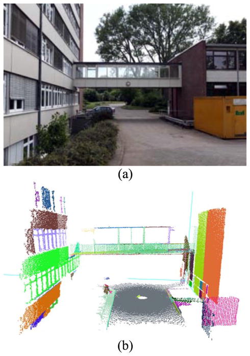
Although the NCC-RANSAC method is devised for extracting planes from the SR4000’s range data, it may also be applied to range data segmentation for other type of range sensors for robotic and computer vision applications. To demonstrate its practical use in segmenting LIDAR data, we ran the NCC-RANSAC on the data [14] collected from a 2-D laser scanner–UTM-30LX. The result is depicted in Fig. 18. It can be seen that the method successfully extracted both large and small planar surfaces. A closer look into the details of the extracted planes finds that these planes are of high quality due to the lower noise of the data.
Fig. 18.
Segmentation of NCC-RANSAC on LIDAR data. (a) Snapshot of the scene. (b) 3-D view (point cloud) of the extracted planes.
VIII. Conclusion
We have presented a new PE method, called NCC-RANSAC, for range data segmentation. The method employs a RANSAC plane-fitting procedure to maximize the number of inlier data points. It then checks normal coherence of the data points and removes those points whose normals are in conflict with that of the fitted plane. This results in a number of separate inlier patches, each of which is then used to extract the corresponding plane through an iterative plane clustering process. The entire NCC-RANSAC is repeated on the range data until all significant planes are found. The method uses one RANSAC plane-fitting procedure to extract multiple planes and is thus more computationally efficient than the CC-RANSAC algorithm. As the proposed method uses both normal and distance criteria to extract a plane from an inlier patch, the resulted planes are free of the over-extraction problem of the existing RANSAC method and its variants and are therefore of better quality. A probabilistic model is proposed to analyze the NCC-RANSAC’s robustness to range data noise and predict the success rate in extracting a plane. The model has been validated by the SR4000’s range data. The experimental results demonstrate that the NCC-RANSAC method has a very high rate of success (close to 100%) in PE.
The method can also be applied to range data segmentation for other type of sensors. It has high parallelism and is suitable for parallel computing. In the future, GPU implementation may be adopted to speed up the method for real-time onboard execution.
Acknowledgments
This work was supported in part by the NSF under Grant IIS-1017672, in part by the National Institute of Biomedical Imaging and Bioengineering and the National Eye Institute of the NIH under Award R01EB018117, and in part by NASA under Award NNX13AD32A.
Biographies

Xiangfei Qian (SM’14) received the B.S. degree in computer science from Nanjing University, Nanjing, China, in 2011. He is currently pursuing the Ph.D. degree from the Department of Systems Engineering, University of Arkansas at Little Rock, Little Rock, AR, USA.
His current research interests include 2-D/3-D computer vision, pattern recognition, and image processing.

Cang Ye (S’97–M’00–SM’05) received the B. E. and M. E. degrees from the University of Science and Technology of China, Hefei, China, in 1988 and 1991, respectively, and the Ph.D. degree from the University of Hong Kong, Hong Kong, in 1999.
From 1999 to 2001, he was a Research Fellow at the School of Electrical and Electronic Engineering, Nanyang Technological University, Singapore. He was also a Research Fellow from 2001 to 2003, and a Research Faculty from 2003 to 2005 with the Advanced Technologies Laboratory, University of Michigan, Ann Arbor, MI, USA. He was an Assistant Professor from 2005 to 2010 with the Department of Applied Science, and has also been an Associate Professor from July 2010 with the Department of Systems Engineering, University of Arkansas at Little Rock, Little Rock, AR, USA. His current research interests include mobile robotics, intelligent system, and computer vision.
Dr. Ye is a member of the Technical Committee on Robotics and Intelligent Sensing and IEEE Systems, Man, and Cybernetics Society.
Footnotes
The content is solely the responsibility of the authors and does not necessarily represent the official views of the funding agencies. This paper was recommended by Associate Editor Q. Ji.
Contributor Information
Xiangfei Qian, Email: xxqian@ualr.edu.
Cang Ye, Email: cxye@ualr.edu.
References
- 1.Ye C. Navigating a mobile robot by a traversability field histogram. IEEE Trans Syst, Man, Cybern B, Cybern. 2007 Apr;37(2):361–372. doi: 10.1109/tsmcb.2006.883870. [DOI] [PubMed] [Google Scholar]
- 2.Ye C, Borenstein J. Obstacle avoidance for the Segway Robotic Mobility Platform. Proc ANS Int Conf Robot Rem Syst Hazard Environ; Gainesville, FL, USA. 2004; pp. 107–114. [Google Scholar]
- 3.Lu X, Manduchi R. Detection and localization of curbs and stairways using stereo vision. Proc. IEEE ICRA; 2005; pp. 4648–4654. [Google Scholar]
- 4.Kinect for Xbox 360. [Online]. Available: http://www.xbox.com/en-US/KINECT.
- 5.Specification of SwissRanger SR4000. [Online]. Available: http://www.mesa-imaging.ch/prodview4k.php.
- 6.Suttasupa Y, Sudsang A, Niparnan N. Plane detection for Kinect image sequences. Proc. IEEE Int. Conf. ROBIO; Phuket, Thailand. 2011; pp. 970–975. [Google Scholar]
- 7.Endres F, Hess J, Engelhard N. An evaluation of the RGB-D SLAM system. Proc. IEEE Int. Conf. Robot. Autom; Saint Paul, MN, USA. 2012; pp. 1691–1696. [Google Scholar]
- 8.Henry P, Krainin M, Herbst E, Ren X, Fox D. RGB-D mapping: Using depth cameras for dense 3D modeling of indoor environments. Proc. ISER; Berlin, Germany. 2010. [Google Scholar]
- 9.Ye C. Navigating a portable robotic device by a 3D imaging sensor. Proc. IEEE Sensors Conf; Kona, HI, USA. 2010; pp. 1005–1010. [Google Scholar]
- 10.Ye C, Bruch M. A visual odometry method based on the SwissRanger SR-4000. Proc. Unmanned Syst. Tech. XII Conf. SPIE DSS; Orlando, FL, USA. 2010. [Google Scholar]
- 11.Jiang X. An adaptive contour closure algorithm and its experimental evaluation. IEEE Trans Pattern Anal Mach Intell. 2000 Nov;22(11):1252–1265. [Google Scholar]
- 12.Fan T, Medioni G, Nevatia R. Segmented description of 3D surfaces. IEEE Trans Robot Autom. 1987 Dec;3(6):527–538. [Google Scholar]
- 13.Kaushik R, Xiao J, Joseph S, Morris W. Fast planar clustering and polygon extraction from noisy range images acquired in indoor environments. Proc. IEEE ICMA; Xi’an, China. 2010; pp. 483–488. [Google Scholar]
- 14.Xiao J, Adler B, Zhang J, Zhang H. Planar segment based three-dimensional point cloud registration in outdoor environments. J Field Robot. 2013;30(4):552–582. [Google Scholar]
- 15.Poppinga J, Vaskevicius N, Birk A, Pathak K. Fast plane detection and polygonalization in noisy 3D range images. Proc. IEEE/RSJ Int. Conf. IROS; Nice, France. 2008; pp. 3378–3383. [Google Scholar]
- 16.Xiao J, Zhang J, Zhang J, Zhang H, Hildre HP. Fast plane detection for SLAM from noisy range images in both structured and unstructured environments. Proc. IEEE ICMA; Beijing, China. 2011; pp. 1768–1773. [Google Scholar]
- 17.Hegde GM, Ye C. Extraction of planar features from SwissRanger SR-3000 range images by a clustering method using normalized cuts. Proc. IEEE/RSJ Int. Conf. IROS; St. Louis, MO, USA. 2009; pp. 4034–4039. [Google Scholar]
- 18.Hoover A, et al. An experimental comparison of range image segmentation algorithms. IEEE Trans Pattern Anal Mach Intell. 1996 Jul;18(7):673–689. [Google Scholar]
- 19.Min J, Powell M, Bowyer KW. Automated performance evaluation of range image segmentation algorithms. IEEE Trans Syst, Man, Cybern B, Cybern. 2004 Feb;34(1):263–271. doi: 10.1109/tsmcb.2003.811118. [DOI] [PubMed] [Google Scholar]
- 20.Hegde GM, Ye C, Anderson GT. Robust planar feature extraction from SwissRanger SR-30000 range images by an extended normalized cuts method. Proc. IEEE Int. Conf. IROS; 2010; pp. 1190–1195. [Google Scholar]
- 21.Bellon O, Direne A, Silva L. Edge detection to guide range image segmentation by clustering techniques. Proc. IEEE ICIP; Kobe, Japan. 1999; pp. 725–729. [Google Scholar]
- 22.Gotardo PFU, et al. Range image segmentation into planar and quadric surfaces using an improved robust estimator and genetic algorithm. IEEE Trans Syst, Man, Cybern B, Cybern. 2004 Dec;34(6):2303–2315. doi: 10.1109/tsmcb.2004.835082. [DOI] [PubMed] [Google Scholar]
- 23.Nurunnabi A, Belton D, West G. Robust segmentation for multiple planar surface extraction in laser scanning 3D point cloud data. Proc. ICPR; Tsukuba, Japan. 2012; pp. 1367–1370. [Google Scholar]
- 24.Nurunnabi A, Belton D, West G. Robust segmentation in laser scanning 3D point cloud data. Proc. DICTA; Fremantle, WA, Australia. 2012; pp. 1–8. [Google Scholar]
- 25.Borrmann D, Elseberg J, Lingemann K, Nüchter A. The 3D Hough Transform for plane detection in point clouds—A review and a new accumulator design. J 3D Res. 2011 Mar;2(2):Article 32. [Google Scholar]
- 26.Fleishman S, Cohen-Or D, Silva CT. Robust moving least-squares fitting with sharp features. ACM Trans Graph. 2005;24(3):544–552. [Google Scholar]
- 27.Fischler MA, Bolles RC. Random sample consensus: A paradigm for model fitting with applications to image analysis and automated cartography. Commun ACM. 1981;24(6):381–395. [Google Scholar]
- 28.Model Fitting and Robust Estimation: RANSAC Algorithm. [Online]. Available: http://www.csse.uwa.edu.au/~pk/research/matlabfns.
- 29.Gallo O, Manduchi R, Rafii A. CC-RRANSAC: Fitting planes in the presence of multiple surfaces in range data. Pattern Recognit Lett. 2011;32(4):403–410. [Google Scholar]


