Using high-resolution satellite aerosol optical depth to estimate daily PM_2.5 geographical distribution in Mexico City

Abstract

Recent advances in estimating fine particle (PM_2.5) ambient concentrations use daily satellite measurements of aerosol optical depth (AOD) for spatially and temporally resolved exposure estimates. Mexico City is a dense megacity that differs from other previously modeled regions in several ways: it has bright land surfaces, a distinctive climatological cycle, and an elevated semi-enclosed air basin with a unique planetary boundary layer dynamic. We extend our previous satellite methodology to the Mexico City area, a region with higher PM_2.5 than most US and European urban areas. Using a novel 1 km resolution AOD product from the MODIS instrument, we constructed daily predictions across the greater Mexico City area for 2004–2014. We calibrated the association of AOD to PM_2.5 daily using municipal ground monitors, land use, and meteorological features. Predictions used spatial and temporal smoothing to estimate AOD when satellite data were missing. Our model performed well, resulting in an out-of-sample cross validation R² of 0.724. Cross-validated root mean squared prediction error (RMSPE) of the model was 5.55 μg/m³. This novel model reconstructs long- and short-term spatially resolved exposure to PM_2.5 for epidemiological studies in Mexico City.

Introduction

Mexico City is a megacity, with a population of more than 24 million. Air pollution is a major public health threat, particularly in the urban regions of Mexico. The Mexican National Institute of Statistics and Geography estimates that the total cost of atmospheric contamination was 3.4% of national GDP in 2012.¹ Effective quantitation of exposure to air pollution for epidemiologic studies and policy analysis requires measurements that go beyond the relatively sparse air monitoring network to more finely capture the exposure variability that may be driving health effects. Mexico City’s unique geography, climate, and demography contribute to the high levels of air pollution. The city sits in an elevated basin, 2240 m above sea level and surrounded on three sides by mountain ridges, but with a broad opening to the north and a narrower gap to the south-southeast. There are over 40,000 industries and >5.5 million vehicles passing through the city daily. The combined high altitude and tropical insolation contribute to incomplete combustion and the formation of secondary particulate matter (PM). Air quality is generally worse in the winter, when rain is less common and thermal inversions are more frequent.^{2, 3} These distinctive characteristics also make modeling air pollution in Mexico City challenging.

Until recent years, epidemiologic studies on the health effects of PM have used exposure estimates with limited geospatial information (such as central ground monitors), assigning measurements to populations within a specified distance of the monitor.^{4, 5} These types of exposure assignment methods have been used in studies of the health impacts of air pollution in Mexico City.^6–8 This exposure assignment method can introduce error and most likely biases the effect estimates downward due to spatial misalignment.⁹ To address this exposure misclassification, various tools have been developed over the past few years.^10–13 A commonly used approach is land use regression (LUR), which uses geographic covariates to expand in situ measurements of PM_2.5 concentrations to large areas. Unfortunately, because these geographic covariates are mostly non-time varying, the temporal resolution of most LUR models is limited and these types of exposure models are used mainly to assess chronic health effects. Recent improvements of LUR address some of its inherent limitations.^14–16 Some of these approaches use newly available satellite data to greatly expand the temporal variability as well as spatial coverage of LUR. Satellite-based aerosol optical depth (AOD) is a derived geophysical daily measurement that can be used to estimate air quality and pollution. AOD is a measure of the scattering/extinction of electromagnetic radiation at a given wavelength due to the presence of aerosols in the atmospheric column. Chang and colleagues have used new statistical downscaling and data fusion techniques to predict PM_2.5 concentrations at spatial point locations in the southeastern United States during the period 2003–2005 using MODIS (Moderate Resolution Imaging Spectroradiometer) satellite data.¹⁷ Their model performed well in cross-validated predictions (R²=0.78 and a root mean-squared error (RMSE) of 3.61 μg/m³). Similarly, Chudnovsky and colleagues¹⁸ used one year of observations from the newly developed Multi-Angle Implementation of Atmospheric Correction (MAIAC) algorithm based on MODIS.^{19, 20} They used AOD data at 1 km spatial resolution to generate daily PM_2.5 estimates for co-located AOD and PM_2.5 sites. The model predictive performance spatially was similar to that estimated by Chang et al. (spatial R²=0.79). More recently, our group used high resolution MAIAC data to develop models to predict daily PM_2.5 at a 1*1 km resolution across the entire northeastern USA for the years 2003–2011 which allowed us to better differentiate daily and long term exposure between urban, suburban, and rural areas.²¹ Our model performance improved upon these initial breakthroughs in satellite based modeling (cross-validated predictions R²=0.88). In addition, our results revealed very low bias (slope of predictions versus withheld observations of 0.99), which suggests that residual error in estimates from this approach will be non-differential.

Although demonstrated successfully in the northeastern USA, it remains uncertain how well the hybrid-satellite approach would perform in areas that are significantly different from the northeastern USA in geography, climate, and PM characteristics. Other groups have used lower resolution (~10km) AOD products in estimating the global burden of disease, including estimating PM_2.5 long term averages over Mexico City, but have not tailored the fit for daily predictions.²² A number of geographic features distinguish the Mexico City metropolitan area (MCMA) from other areas in which hybrid models have been generated, particularly in the northeastern USA. Differences include the meteorological patterns and seasonality, the semi-enclosed basin confining regional pollution, the higher elevation and consequent less efficient motor vehicle combustion. In addition, Mexico City has brighter land surfaces related to surface soils, limited vegetation, and prevalent building materials, which contributes to error in the derivation of the satellite AOD estimates. These physical/meteorological differences, the additional error in the AOD estimates, as well as limited data availability on local pollution sources (such as traffic density or roadway classifications) in the Mexico City region add to the challenge of generating PM_2.5 prediction models. The goal of this paper was to use the new MAIAC AOD satellite data to estimate PM_2.5 in the MCMA adapting and extending the previous hybrid-model approach to account for the unique challenges of the Mexico City region.

Methods

Study Area

The study area included the region of Mexico City within longitude −99.42 to −98.67 and latitude 19.09 to 19.77. To avoid making predictions in the largely uninhabited outlying mountains to the south west and east of the city, the study area was restricted to the contiguous Mexico City valley area of topologically connected grid cells with elevation less than 3000 meters using the mean elevation within each 1 km grid cell from the ASTER GDEM V2.²³ The resulting region included 4694 1 km grid cells.

AOD Data

Daily MAIAC spectral AOD was derived from MODIS Aqua Collection 6 L1B data for the period of 2004–2014. MAIAC algorithm provides a high resolution (1 km) AOD product that was used in our analysis for the Mexico City area. The MAIAC data from MODIS Aqua represent a midafternoon measurement (mean daily acquisition time of 2:57pm GMT -5 hours; range 2:10–3:45pm local overpass time). An in depth description of the MAIAC product and algorithm details can be found in previous publications.^{19, 20} Because AOD values may be spurious at cloud edges, AOD data were filtered to exclude values with adjacent cloud or high uncertainty flags, and with a moving window variance in the top 2.5th percentile. The resulting MAIAC dataset included 19.8% of all possible observations which is consistent with our previous work in the New England region.²¹

Monitoring data

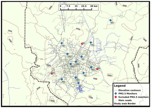
Data for daily PM_2.5 mass concentrations across Mexico City for the study period (January 2, 2004 to April 30, 2014) were downloaded from the automated air quality monitoring network of Mexico City (RAMA).²⁴ Daily PM_2.5 concentrations were calculated as the mean of the hourly measurements (≥18 available) collected on tapered element oscillating microbalance (TEOM) devices. The Atmospheric Monitoring System of Mexico City (SIMAT) also provided monitor locations and meteorological network data including temperature and relative humidity which were assigned based on the closest available station (e.g. from 23 stations reporting temperature). We analyzed local features of monitor locations and saw that specific locations had much lower MAIAC retrieval. For example, in the grid cell containing the station “PER”, the surface brightness analyzed by the MAIAC algorithm was 30–50% brighter than at the other sites making the MAIAC data less reliable in these locations. Due to these features, three monitors in atypical locations were excluded leaving a total of 12 monitors used in the remaining analyses (all locations shown in Figure 1). Measurements from Christmas and New Years included many outlying values, potentially associated with the use of fireworks. These two dates include 18 of the 20 highest monitor-day observations in the dataset and were excluded from model calibration.

Figure 1.

Map of the study area showing the border of the AOD grid, the location of the PM_2.5 monitoring stations, major roadways, and elevation contours.

Spatial and Temporal Predictors of PM_2.5

The multi-step regression modeling approach included AOD, classic land use predictors and temporal predictors. Spatial covariates were generated using ArcMap version 10.2 and mapped with QGIS version 2.8.^{25, 26} All spatial data were projected into UTM zone 14N. We used the following spatial predictors:

Roadway density

Roadway data were obtained from OpenStreetMap (downloaded July 31, 2013; openstreetmap.org).²⁷ Total road density was calculated using the line density tool in the ArcGIS spatial analyst toolbox. This calculates the total polyline distance of all roads per square kilometer around the centroids of the satellite AOD cells across the study area. We used the following temporal predictors:

Meteorological data

Temperature and relative humidity were obtained from the SIMAT except for 100 days of relative humidity in 2007 that were missing from the SIMAT database and were imputed using the airport meteorological station. Grid cells were matched to the closest weather station with available daily means for these variables (≥18 hourly measurements).

Planetary boundary layer

Hourly PBL (mixing height) measurements between 6:00 and 18:00 from a fixed site within the city were provided by the Secretaría del Medio Ambiente²⁸ and included in the model as the mean of the morning measurements. The height of the boundary layer may vary with local meteorological conditions, influencing the concentration and vertical profile of pollutants. The boundary layer not only controls transport and location of pollutants and aerosols but also their concentrations would be different in variable boundary layer structures.²⁹

Daily precipitation

Daily precipitation measurements (in mm) were entered as a daily citywide mean obtained through Sistema de Aguas de la Ciudad de México.³⁰

Population at risk estimates

Demographic data were obtained from the 2010 Mexican National Census.³¹ We calculated the average population for each 1 km grid cell centroid based on the census statistical areas (AGEBs) intersecting these grid cells.

Statistical Methods

All modeling was done using the R statistical software version 3.2.0.³² In the Mexico City area there are large day-to-day differences in mean PM_2.5 concentration, PBL, temperature, and precipitation. These daily differences create a varying relationship between the AOD surface and PM_2.5 for every single day and thus we chose to use a mixed effects model as we have done in some of our previous studies.^{21, 33, 34} We incorporate spatial and temporal predictors and day-specific random-effects to account for these temporal variations in the PM_2.5–AOD relationship. To generate the daily 1 km PM_2.5 predictions in each grid cell for the entire period, we developed an analytic process as follows:

The first stage calibrates the AOD grid-level observations to the PM_2.5 monitoring data using all monitor-day observations with the closest available AOD value within 1.1 km during the study period, while adjusting for spatial and temporal covariates. Specifically, we fit the following model (calibration stage):

$$\begin{array}{l}{\text{PM}}_{\text{ij}}=(\mathrm{\alpha }+{\mathrm{u}}_{\mathrm{j}})+({\mathrm{\beta }}_1+{\mathrm{v}}_{\mathrm{j}}){\text{AOD}}_{\text{ij}}+{\mathrm{\beta }}_2{\text{Temperature}}_{\text{ij}}+{\mathrm{\beta }}_3\text{Relative}{\text{Humidity}}_{\text{ij}}+{\mathrm{\beta }}_4\text{Mean}\text{AM}{\text{PBL}}_{\mathrm{j}}+{\mathrm{\beta }}_5\surd {\text{Precipitation}}_{\mathrm{j}}+{\mathrm{\beta }}_6\text{Roadway}{\text{density}}_{\mathrm{i}}+{\mathrm{\epsilon }}_{\text{ij}}\\ ({\mathrm{u}}_{\mathrm{j}}{\mathrm{v}}_{\mathrm{j}})~[(0,0),\mathrm{\sum }]\end{array}$$

Where: PM_ij denotes the measured PM_2.5 concentration at a spatial site i on a day j; α and u_j are the fixed and random daily intercepts, respectively, AOD_ij is the AOD value in the grid cell corresponding to site i on day j; β₁ and v_j are the fixed and random slopes, respectively. Temperature_ij and Relative Humidity_ij are the assigned closest available values in the grid cells corresponding to site i on a day j. Mean AM PBL_j and Precipitation_j are the values on date j. Roadway density_i is the mean in the grid cell containing site i. Finally, Σ is an unstructured variance-covariance matrix for the random effects.

Following this process we predicted daily PM_2.5 concentrations in grid cells without monitors but with available AOD measurements using the calibration stage model coefficients. This resulted in PM_2.5 prediction for all day-grid cell combinations with available satellite based AOD.

In the second stage (full coverage model), in order to predict daily PM_2.5 in grid cells with no AOD on that day across the study area, we make use of the city-wide association between grid-cell AOD and PM_2.5 levels, and the association between PM_2.5 level in a given grid cell with that in neighboring grid cells. Since the spatial pattern of air pollution varies by season we fit a separate smooth spatial surface for each season (cold-dry: November-February; warm-dry: March-April; and rainy: May-October) across the study time period.² To constrain this surface to positive variation around the time series, the full coverage model was fit on the square root of the calibration stage predictions and subsequently back transformed. Specifically, we fit the following model (full coverage stage):

$$\surd {\text{PredPM}}_{\text{ij}}=\mathrm{\alpha }+{\mathrm{\beta }}_1\surd {\text{MPM}}_{\mathrm{j}}+\mathrm{s}{({\mathrm{X}}_{\mathrm{i}},{\mathrm{Y}}_{\mathrm{i}})}_{\mathrm{k}(\mathrm{j})}+{\mathrm{\epsilon }}_{\text{ij}},$$

where PredPM_ij is the predicted PM_2.5 concentration at a grid cell i on a day j from the first stage fit; MPM_j is the mean PM across all monitors in the MCMA on a day j; α is the intercept, β₁ is the slope for the daily mean. The terms X_i,Y_i are the longitude and latitude, respectively, of the centroid of grid cell i, and s(X_i,Y_i) _k(j) is a generalized additive model using a tensor product of cubic regression splines specific to the seasonal period k(j) in which day j falls. To allow for differences over time this model is fit separately for each of the 32 seasonal periods.

Model performance was assessed using monitor-level leave-one-out cross-validation. Each monitor was withheld and predictions were aggregated from refitting the model 12 times. To test our results for bias, we regressed the measured PM_2.5 concentration for a given monitor and day against the corresponding predicted value generated without the use of that monitor. We estimated the model prediction precision by taking the square root of the mean squared prediction errors (RMSPE), which are reported in units of μg/m³.

Results

There were 12 included PM_2.5 monitors with unique locations operating across the city during the study period (Figure 1). Monitors were brought online at various dates and had measurements available for a median of 90% (range of 76% to 94%) of days between their deployment and their decommission date or the end of the study period. The mean daily PM_2.5 across the city during the study period at these monitors was 25.3 μg/m³ with a standard deviation of 10.3 μg/m³ and an interquartile range (IQR) of 17.8–31.5 μg/m³. Pearson correlations comparing pairs of monitors on days they were both running range from 0.69 to 0.93 (median 0.85) and were not substantively different from Spearman correlations.

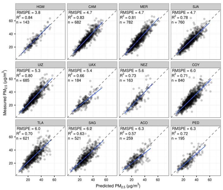
The calibration (stage 1) model presented high cross-validated fits across the entire study period, with a cross-validated R² of 0.729, and as expected, a highly significant association between PM_2.5 and the main explanatory variable AOD, which had the largest t-value of the calibration model covariates (Table 1). The cross-validated RMSPE of calibration fits was 5.42 μg/m³, which is less than the observed variability in PM_2.5 concentrations in the MCMA. The fit of the calibration stage varied across monitors and across time, with generally worse fits in the earlier years of the model and at monitoring stations further from the center of the region. Figure 2 shows the cross-validated predictions versus observations at each monitor. Subsetting by year, the predictions have been improving from the largest RMSPE of 6.3 μg/m³ in 2004 to the best fits in 2012 and 2014 of 4.5 and 4.6 μg/m³, respectively.

Table 1.

Calibration Model Regression Fixed Effects

	Estimate	Std. Error	t value	p-value
(Intercept)	12.94	1.35	9.60	< 2e-16
AOD	14.41	0.93	15.53	< 2e-16
Temperature	0.58	0.07	8.88	< 2e-16
Relative Humidity	0.12	0.02	7.97	2.0e-15
Mean AM PBL/100	−1.72	0.13	−12.92	< 2e-16
√Precipitation	−4.85	0.66	−7.33	4.1e-13
Roadway density	0.21	0.01	14.06	< 2e-16

Figure 2.

Calibration stage cross-validation predictions versus measurements at 12 monitors in Mexico City, 2004–2014.

The full coverage model also performed very well with a mean cross-validated R² of 0.724 (fit on the same dataset as the calibration model), which is relatively high considering that this model makes a prediction at all day-locations even if satellite AOD are not available. The cross-validated RMSPE of the full coverage model was 5.55 μg/m³, which was only slightly larger than the calibration stage. Predictions had little bias with cross-validated slopes (predicted versus observed) of 1.00 ± 0.008 s.e. and 1.12 ± 0.009 s.e., respectively, in the calibration and full coverage stages. As shown in Figure 3, the cross-validated model predictions from the full coverage stage are better on the non-Holiday dates although those two peak days (Christmas and New Years) account for many of the highest PM_2.5 concentrations in Mexico City which may be related to the use of fireworks and other abnormal pollution events.

Figure 3.

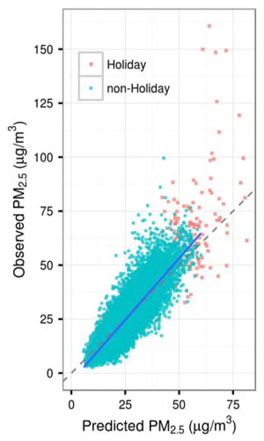
Cross-validated predictions from the full coverage model versus measurements at the 12 monitoring stations. The blue line is a generalized additive model fit to the subset of points that are not Christmas or New Years. The dashed grey line represents the one-to-one diagonal.

Figure 4 presents the ground level PM_2.5 and our cross-validated predictions from the full coverage model for a representative monitor, “CAM”, located in the middle of the city, for the year 2010. As can be seen in the figure there is an excellent agreement between the ground level PM_2.5 measurements and our cross-validated predictions.

Figure 4.

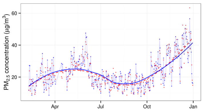
PM_2.5 measurements and cross-validated predictions from the full coverage model for the CAM monitor in 2010. Connected blue points are the daily PM_2.5 measurements while red points are the full coverage predictions. Smoothed curves are loess regression lines for measurements (solid) and predictions (dashed).

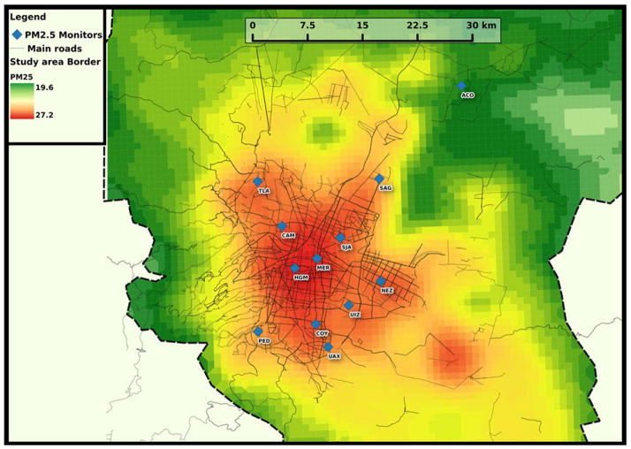
Figure 5 shows the spatial pattern of PM_2.5 predictions averaged over the entire study period. Mean predicted PM_2.5 concentrations range from 19.7 μg/m³ to 27.2 μg/m³, showing substantial spatial variability across the region even in the long-term average of the daily predictions. By superimposing the fine scale predictions on 2010 census units (AGEBs), we generate an estimate of the population at risk over this study period. While there is considerable variability in the estimated long-term PM_2.5 exposures, 50% of the population in this greater Mexico City area is exposed to at least 24.1 μg/m³ mean daily PM_2.5, which is far in excess of the new PM_2.5 Mexican Air Quality Standards (AQS) for annual averages of 12 μg/m³ as referenced by Calderón-Garcidueñas.⁷

Figure 5.

The overall mean of daily 1 km PM_2.5 predictions for all years (2004–2014) across the Mexico City region

Discussion

To our knowledge we have developed the first high spatially and temporally resolved PM_2.5 exposure model for the Mexico City Metropolitan Area for a decadal period (2004–2014). Using satellite measurements, we developed and validated models to predict daily PM_2.5 at a 1*1 km resolution across the large megacity region of the MCMA, allowing us to differentiate daily and long-term intra city exposure. Perhaps most importantly we have demonstrated the robustness of high-resolution satellite-based PM models by expanding their use into populated regions with unique features that required refinement of previous approaches. We have shown excellent model performance in a region that is challenging to model given the unique geographical and climatological characteristics of the MCMA. Our model building suggested that planetary boundary layer and precipitation data were important predictors in this region and that the model fit was improved through additional preprocessing of MAIAC datasets, perhaps because of the underlying bright surfaces and cloud detection/mask characteristics in this region. The resulting daily predictions on a 1*1 km grid offer exposure metrics for acute and chronic health outcome analyses in this understudied but highly exposed megacity. Finally, given the large population at risk (>9 million with more than 24.1 μg/m³ average PM_2.5 over 2004–2014), this daily exposure model will have great impact in studying acute and chronic associations of air pollution with consequent morbidity and mortality in the MCMA. Because this model can objectively capture spatially resolved PM_2.5 exposure for a 10 year period, the potential uses when linked to public health and research databases that cover the same time frame will be enormous.

The model allows the comparison of temporal trends across the region with those previously described for the monitoring locations alone.⁷ Calderón-Garcidueñas and colleagues note that there is no clear downtrend in PM_2.5 at the RAMA monitoring stations. In line with this study, when exploring our PM_2.5 predictions temporally (Figure 6), the highest mean concentrations were at the start of our study period but fluctuate in recent years without a clear temporal trend. Also in line with the analysis of Calderón-Garcidueñas at the monitoring stations, we note that there was a slight decrease in the predictions for the year 2010 relative to the years before and after.

Figure 6.

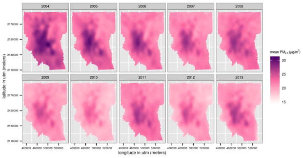
Temporal trends in annual mean daily PM_2.5 predictions across the Mexico City region showing 10 complete years (2004–2013).

Our approach has several new refinements over previous methods. Relative to previously available exposure modeling approaches in the MCMA,⁶ our model allows daily estimates even in areas within the city that are not adjacent to the few stationary municipal monitors. One potential application would be to determine locations in the MCMA in which the existing monitoring is not in agreement with our predictions in order to prioritize sites for additional monitors. Although reconstructed after collection, these prospective measurements are objective exposure estimates that go back a decade. Thus, this model is particularly well suited for use in epidemiologic studies including cohorts and national health surveys that collected residence data and took place from 2004 to 2014 anywhere within this geographic region.

Our model is subject to several limitations, some of which apply to all indirect exposure estimation methods. First, this model relies on a relatively small network of ground monitors and this limits the ability to consider how spatial covariates modify the association of AOD and ground level PM_2.5. Although we add in satellite measurements of AOD, the satellite measurements reflect particles in the entire air column and these data need to be calibrated against the ground concentrations before use in predictions to capture air levels within the population’s “breathing zone”. Our 1 km resolution predictions are the finest resolution of AOD data that have been produced to date. Even though our model has almost 5000 daily predictions over this urban region, and 100x the areal density of the more commonly used 10*10 km approach, it still may not capture very local effects such as residing directly next to a high traffic roadway. Future models may incorporate these very local effects in a third-stage LUR, as was recently applied in the Northeastern United States.²¹ Similarly, this model may not capture aberrant pollution events such as the fireworks associated with PM_2.5 spikes on Christmas and New Year days. The inclusion of additional co-pollutants may also improve the model fit by adjusting for how source emissions patterns alter the AOD-PM association. A major limitation in satellite-based approaches is that measurements are unavailable when they are obscured by clouds. Mexico City is particularly challenging because the rainy season can lead to prolonged periods with low satellite coverage. Our model exploits the correlation of PM in this region by smoothing to cover missing satellite data. Our cross-validation approach, in which each monitor is completely excluded from model fits in turn, serves as a useful check on the prediction accuracy for the exposure model at the monitoring locations which is akin to checking our model if we had an epidemiologic study participant living at that location. However, the limited scale and non-independence of the underlying monitor network limits the number of checks that we have on the resulting predictions. Another limitation of developing these models in new regions is the availability and quality of local geospatial data to characterize sources of pollution such as emissions from traffic. This model uses the density of roadways as estimated from OpenStreetMap, which is similar to metrics commonly used in many published LUR studies. This metric could likely be improved with additional data on the road type, classification, size, and traffic volume for each road segment. Unfortunately we were unable to procure more detailed traffic or roadway data for this model, which is part of the challenge of developing these modeling approaches in new regions.

Because our model uses physical measurements from the satellite, it cannot be used to forecast future exposure levels and thus the benefit for environmental policy may be primarily through understanding past and current patterns of exposure. However, the model may be quite useful in quantifying the impacts of previous public health interventions on air pollution reduction, and in epidemiologic studies of acute and chronic health effects. Ideal exposure assessment for epidemiologic health studies would entail continuous personal exposure monitoring. However, personal monitoring is not logistically feasible for large populations and can only be collected prospectively. The use of a prediction model as we present here is dependent on accurate residential history and geocoding and will not capture exposure events that happen exclusively indoors (e.g. cooking) or in other microenvironments (e.g. inside vehicles). However, the open architecture and low prevalence of air conditioning in Mexico City means that outdoor air pollution easily mixes with indoor air and our model is likely a reasonable estimate of pollution exposure in the home minus these additional sources.

Future iterations of this model will benefit from further developments of the MAIAC algorithm to derive AOD over brighter surfaces and from increased frequency of observations by combining MODIS data from NASA’s Terra and Aqua satellites. We are working on new modeling approaches that augment seasonal patterns of sparse MAIAC coverage with multi-level satellite data, emissions-based exposure models, and novel geostatistical methods. In addition, it may be possible to expand this approach to other regions of Mexico, particularly in the larger Megalopolis (the region including the MCMA and surrounding states) utilizing additional municipal ground monitoring networks.

References

- 1.INEGI (Instituto Nacional de Estadística y Geografía) Sistema de Cuentas Nacionales de México : cuentas económicas y ecológicas de México. 2012 http://www.inegi.org.mx/prod_serv/contenidos/espanol/bvinegi/productos/derivada/economicas/medio_ambiente/MONOGRAFIA_SCEEM_2012.pdf.
- 2.De Foy B, Caetano E, Magana V, Zitácuaro A, Cárdenas B, Retama A, Ramos R, Molina LT, Molina MJ. Mexico City basin wind circulation during the MCMA-2003 field campaign. Atmospheric Chemistry & Physics. 2005;5:2267–2288. [Google Scholar]
- 3.Molina LT, Madronich S, Gaffney J, Apel E, Foy Bd, Fast J, Ferrare R, Herndon S, Jimenez JL, Lamb B, et al. An overview of the MILAGRO 2006 Campaign: Mexico City emissions and their transport and transformation. Atmospheric Chemistry and Physics. 2010;10:8697–8760. [Google Scholar]
- 4.Laden F, Schwartz J, Speizer FE, Dockery DW. Reduction in fine particulate air pollution and mortality: extended follow-up of the Harvard Six Cities study. American journal of respiratory and critical care medicine. 2006;173:667–672. doi: 10.1164/rccm.200503-443OC. [DOI] [PMC free article] [PubMed] [Google Scholar]
- 5.Ebelt ST, Wilson WE, Brauer M. Exposure to ambient and nonambient components of particulate matter: a comparison of health effects. Epidemiology. 2005;16:396–405. doi: 10.1097/01.ede.0000158918.57071.3e. [DOI] [PubMed] [Google Scholar]
- 6.Romieu I, Meneses F, Ruiz S, Sienra JJ, Huerta J, White MC, Etzel RA. Effects of air pollution on the respiratory health of asthmatic children living in Mexico City. American journal of respiratory and critical care medicine. 1996;154:300–307. doi: 10.1164/ajrccm.154.2.8756798. [DOI] [PubMed] [Google Scholar]
- 7.Calderon-Garciduenas L, Kulesza RJ, Doty RL, D’Angiulli A, Torres-Jardon R. Megacities air pollution problems: Mexico City Metropolitan Area critical issues on the central nervous system pediatric impact. Environmental Research. 2015;137:157–169. doi: 10.1016/j.envres.2014.12.012. [DOI] [PubMed] [Google Scholar]
- 8.Escamilla-Nunez MC, Barraza-Villarreal A, Hernandez-Cadena L, Moreno-Macias H, Ramirez-Aguilar M, Sienra-Monge JJ, Cortez-Lugo M, Texcalac JL, del Rio-Navarro B, Romieu I. Traffic-related air pollution and respiratory symptoms among asthmatic children, resident in Mexico City: the EVA cohort study. Respiratory research. 2008;9:74. doi: 10.1186/1465-9921-9-74. [DOI] [PMC free article] [PubMed] [Google Scholar]
- 9.Zeger SL, Thomas D, Dominici F, Samet JM, Schwartz J, Dockery D, Cohen A. Exposure measurement error in time-series studies of air pollution: concepts and consequences. Environ Health Perspect. 2000;108:419–26. doi: 10.1289/ehp.00108419. [DOI] [PMC free article] [PubMed] [Google Scholar]
- 10.Vienneau D, De Hoogh K, Beelen R, Fischer P, Hoek G, Briggs D. Comparison of land-use regression models between Great Britain and the Netherlands. Atmospheric Environment. 2010;44:688–696. [Google Scholar]
- 11.Hoek G, Beelen R, de Hoogh K, Vienneau D, Gulliver J, Fischer P, Briggs D. A review of land-use regression models to assess spatial variation of outdoor air pollution. Atmospheric Environment. 2008;42:7561–7578. [Google Scholar]
- 12.Gryparis A, Paciorek CJ, Zeka A, Schwartz J, Coull BA. Measurement error caused by spatial misalignment in environmental epidemiology. Biostatistics (Oxford, England) 2009;10:258–274. doi: 10.1093/biostatistics/kxn033. [DOI] [PMC free article] [PubMed] [Google Scholar]
- 13.Beckerman BS, Jerrett M, Serre M, Martin RV, Lee SJ, van Donkelaar A, Ross Z, Su J, Burnett RT. A hybrid approach to estimating national scale spatiotemporal variability of PM2.5 in the contiguous United States. Environmental science & technology. 2013;47:7233–7241. doi: 10.1021/es400039u. [DOI] [PMC free article] [PubMed] [Google Scholar]
- 14.Sampson PD, Richards M, Szpiro AA, Bergen S, Sheppard L, Larson TV, Kaufman JD. A regionalized national universal kriging model using partial least squares regression for estimating annual PM 2.5 concentrations in epidemiology. Atmospheric Environment. 2013;75:383–392. doi: 10.1016/j.atmosenv.2013.04.015. [DOI] [PMC free article] [PubMed] [Google Scholar]
- 15.Liu Y, Paciorek CJ, Koutrakis P. Estimating Regional Spatial and Temporal Variability of PM2.5 Concentrations Using Satellite Data, Meteorology, and Land Use Information. Environ Health Perspect. 2009;117:886–892. doi: 10.1289/ehp.0800123. [DOI] [PMC free article] [PubMed] [Google Scholar]
- 16.Bergen S, Sheppard L, Sampson PD, Kim SY, Richards M, Vedal S, Kaufman JD, Szpiro AA. A national prediction model for PM2.5 component exposures and measurement error-corrected health effect inference. Environ Health Perspect. 2013;121(9):1017–25. doi: 10.1289/ehp.1206010. [DOI] [PMC free article] [PubMed] [Google Scholar]
- 17.Chang HH, Hu X, Liu Y. Calibrating MODIS aerosol optical depth for predicting daily PM2.5 concentrations via statistical downscaling. J Expo Sci Environ Epidemiol. 2014;24(4):398–404. doi: 10.1038/jes.2013.90. [DOI] [PMC free article] [PubMed] [Google Scholar]
- 18.Chudnovsky AA, Koutrakis P, Kloog I, Melly S, Nordio F, Lyapustin A, Wang Y, Schwartz J. Fine particulate matter predictions using high resolution Aerosol Optical Depth (AOD) retrievals. Atmospheric Environment. 2014;89:189–198. doi: 10.1016/j.atmosenv.2014.07.014. [DOI] [PMC free article] [PubMed] [Google Scholar]
- 19.Lyapustin A, Martonchik J, Wang Y, Laszlo I, Korkin S. Multiangle implementation of atmospheric correction (MAIAC): 1. Radiative transfer basis and look-up tables. Journal of Geophysical Research. 2011;116(D3) [Google Scholar]
- 20.Lyapustin A, Wang Y, Laszlo I, Kahn R, Korkin S, Remer L, Levy R, Reid JS. Multiangle implementation of atmospheric correction (MAIAC): 2. Aerosol algorithm. Journal of Geophysical Research. 2011;116(D3) [Google Scholar]
- 21.Kloog I, Chudnovsky AA, Just AC, Nordio F, Koutrakis P, Coull BA, Lyapustin A, Wang Y, Schwartz J. A new hybrid spatio-temporal model for estimating daily multi-year PM2.5 concentrations across northeastern USA using high resolution aerosol optical depth data. Atmospheric Environment. 2014;95:581–590. doi: 10.1016/j.atmosenv.2014.07.014. [DOI] [PMC free article] [PubMed] [Google Scholar]
- 22.Krzyzanowski M, Apte JS, Bonjour SP, Brauer M, Cohen AJ, Prüss-Ustun AM. Air pollution in the mega-cities. Current Environmental Health Reports. 2014;1(3):185–191. [Google Scholar]
- 23.NASA. METI ASTER Global Digital Elevation Model V2. https://lpdaac.usgs.gov/products/aster_products_table/astgtm.
- 24.SIMAT (Sistema de Monitoreo Atmosferico) http://www.aire.df.gob.mx/
- 25.ESRI. ArcGIS 10.2. ESRI; Redlands, CA: 2013. [Google Scholar]
- 26.QGIS Development Team. QGIS Geographic Information System. Open Source Geospatial Foundation; 2015. [Google Scholar]
- 27.Haklay M, Weber P. OpenStreetMap: User-Generated Street Maps. Pervasive Computing, IEEE. 2008;7(4):12–18. [Google Scholar]
- 28.SMA (Secretaría del Medio Ambiente) 2014 [Google Scholar]
- 29.Oke TR. Boundary layer climates. Routledge: 2002. [Google Scholar]
- 30.SACMEX . Gobierno del Distrito Federal. Vol. 2014 Sistema de Aguas de la Ciudad de México; 2014. Subdirección de Macromedición y Control de Redes. [Google Scholar]
- 31.INEGI (Instituto Nacional de Estadística y Geografía) Censo de Población y Vivienda. 2010 http://www.censo2010.org.mx.
- 32.R Core Team, R. A language and environment for statistical computing. R Foundation for Statistical Computing; Vienna, Austria: 2015. [Google Scholar]
- 33.Kloog I, Koutrakis P, Coull BA, Lee HJ, Schwartz J. Assessing temporally and spatially resolved PM2.5 exposures for epidemiological studies using satellite aerosol optical depth measurements. Atmospheric Environment. 2011;45(35):6267–6275. [Google Scholar]
- 34.Kloog I, Nordio F, Coull BA, Schwartz J. Incorporating local land use regression and satellite aerosol optical depth in a hybrid model of spatiotemporal PM2.5 exposures in the Mid-Atlantic states. Environmental science & technology. 2012;46:11913–11921. doi: 10.1021/es302673e. [DOI] [PMC free article] [PubMed] [Google Scholar]