Magnetic resonance temperature imaging-based quantification of blood flow-related energy losses

Abstract

This study presents a new approach for evaluating bioheat transfer equation (BHTE) models used in treatment planning, control and evaluation of all thermal therapies. First, 3D magnetic resonance temperature imaging (MRTI) data are used to quantify blood flow-related energy losses, including the effects of perfusion and convection. Second, that information is used to calculate parameters of a BHTE model; in this paper the widely used Pennes BHTE. As a self-consistency check, the BHTE parameters are utilized to predict the temperatures from which they were initially derived. The approach is evaluated with finite-difference simulations and implemented experimentally with focused ultrasound heating of an ex vivo porcine kidney perfused at 0, 20 and 40 ml/min (n = 4 each). The simulation results demonstrate accurate quantification of blood flow-related energy losses, except in regions of sharp blood flow discontinuities where the transitions are spatially smoothed. The smoothed transitions propagate into estimates of the Pennes perfusion parameter but have limited effect on the accuracy of temperature predictions using those estimates. Longer acquisition time periods mitigate the effects of MRTI noise, but worsen the effect of flow discontinuities. For the no-flow kidney experiments, the estimates of a uniform, constant Pennes perfusion parameter are approximately zero, and at 20 and 40 ml/min, the average estimates increase with flow rate to 3.0 and 4.2 kg/m³/s, respectively. When Pennes perfusion parameter values are allowed to vary spatially, but remain temporally constant, BHTE temperature predictions are more accurate than when using spatially uniform, constant Pennes perfusion values, with reductions in RMSE values of up to 79%. Locations with large estimated perfusion values correspond to high flow regions of the kidney observed in T1-weighted MR images. This novel, MRTI-based technique holds promise for improving understanding of thermal therapy biophysics and for evaluating biothermal models.

Graphical abstract

3D MR temperature data following focused ultrasound heating are used to quantify energy losses caused by blood flow for evaluation of biothermal models. Results in ex vivo perfused kidney demonstrate that the Pennes model with spatially varying blood flow is up to 79% more accurate at predicting temperatures than when assuming spatially uniform blood flow. This novel process is a step forward from past evaluations, because dynamic 3D temperatures allow for improved spatial and temporal sensitivity in evaluating biothermal models.

Introduction

Blood flow and biothermal modeling

Blood flow plays a significant role in magnetic resonance-guided focused ultrasound (MRgFUS) treatments (1–4) and other thermal therapies (5–8) by drawing energy away from the heated region, lowering temperatures and reducing the therapeutic effects of the applied energy. The increased heating time required to ablate high blood flow regions extends the overall treatment time, which may already be a significant treatment-limiting factor (2–3). The associated accumulation of thermal dose in the near- and far-fields may endanger healthy tissues (9). If achievable, accurate pretreatment predictions of blood flow-related energy losses and temperature distributions would provide clinicians the information necessary to preemptively adjust treatment plans for improved outcomes. Quantifying the effects of blood flow is also crucial to developing and evaluating the bioheat transfer equation (BHTE) models proposed for use in treatment planning, control and evaluation (10–11).

In a generic BHTE used for MRgFUS predictions of the absolute tissue temperature T (°C),

$$\rho c\frac{dT}{dt}={\dot{Q}}_{FUS}+\nabla ·(\mathrm{k}\nabla T)+{\dot{Q}}_m-{\dot{Q}}_{bl},$$ (1)

the tissue thermal properties- thermal conductivity k (W/m/°C), specific heat c (J/kg/°C), and density r (kg/m³)- and the power deposition pattern Q̇_FUS (W/m³) can be accurately determined from noninvasive methods (12–16), published tissue data (17–20), or ultrasound simulation algorithms (21–22). For MRgFUS applications, contributions of the metabolic heat generation rate Q̇_m are insignificant and therefore neglected in this work. Thus, determining the final term of Equation 1 representing blood flow-related energy losses Q̇_bl (W/m³) is the primary challenge when creating and evaluating biothermal models.

This study introduces a novel magnetic resonance temperature imaging (MRTI)-based process for quantifying blood flow-related energy losses and evaluating biothermal models. First, 3D MRTI data are used to quantify Q̇_bl. Those data are then utilized to calculate blood flow parameters of a BHTE model of interest. Finally, the BHTE model parameters are used to check the self-consistency of the model by predicting the temperatures from which they were derived. As an illustrative example, this study examines the widely applied Pennes BHTE (23) through finite-difference thermal simulations and MRgFUS experiments in an ex vivo perfused kidney.

Pennes bioheat transfer equation

In Pennes BHTE, blood flow-related energy losses are commonly characterized as a scalar thermal energy sink,

$${\dot{Q}}_{bl}=w{c}_{bl}(T-T_{ar}),$$ (2)

where w is the Pennes perfusion parameter (kg/m³/s), c_bl is the specific heat of blood (J/kg/°C), and T and T_ar represent the temperature (°C) of the tissue and arterial blood. While several investigators have attempted to formulate better tissue heat transfer models (e.g. 24–27), Pennes BHTE remains the most widely implemented.

Despite its frequent application, there are few experimental evaluations of the Pennes BHTE (23,28–34), all relying upon a small number of discrete thermocouple or thermistor measurements. This paper extends previous efforts by using 3D MRTI to quantify Q̇_bl, determine the Pennes perfusion parameter w, and test the predictive ability of the Pennes BHTE.

Theory

Quantifying blood flow-related energy losses

After the tissue has been heated and the ultrasound turned off, Equation 1 (assuming uniform thermal conductivity) becomes

$$\rho c\frac{d{T}_{\mathit{\text{exp}}}}{dt}=k{\nabla }^2{T}_{\mathit{\text{exp}}}-{\dot{Q}}_{bl},$$ (3)

where exp indicates 3D MRTI data. Since the thermal properties k, ρ, and c can be measured or found in property tables, direct estimates of Q̇_bl can be made since all other terms in Equation 3 are known. However, early attempts to directly estimate Q̇_bl were extremely susceptible to MRTI noise (35). A major source of this noise susceptibility seems to arise from evaluating the Laplacian conduction term k∇²T_exp, which is calculated from each voxel’s noise-influenced temperature and those of six adjacent voxels.

Replacing the Laplacian conduction term through the use of a finite-difference thermal model can mitigate the MRTI noise effects. To illustrate, consider two successive 3D MRTI measurements obtained during the cooling period at time points n and n+1. Using the first experimental temperature distribution, T_n,exp, as an initial condition, the temperature decay for the next MRTI acquisition time interval, Δt_acq, is calculated via finite-difference methods in a pure conduction model,

$$\rho c\frac{d{T}_{\mathit{\text{mod}}}}{dt}=k{\nabla }^2{T}_{\mathit{\text{mod}}}.$$ (4)

Subscript mod is for modeled data.

If the effects of conduction and blood flow are separable for the short time period involved (Δt_acq) (36–37), then

$$k{\nabla }^2{T}_{\mathit{\text{exp}}}=k{\nabla }^2{T}_{\mathit{\text{mod}}},$$ (5)

and Equation 3 becomes

$$\rho c\frac{d{T}_{\mathit{\text{exp}}}}{dt}=\rho c\frac{d{T}_{\mathit{\text{mod}}}}{dt}-{\dot{Q}}_{bl},$$ (6)

wherein the noisy Laplacian conduction term has been replaced by a smoother, modeled temperature term, $\rho c\frac{d{T}_{\mathit{\text{mod}}}}{dt}$.

Time derivatives in Equation 6 are approximated using Δt_acq, temperature changes from consecutive experimental measurements (ΔT_exp = T_n+1,exp − T_n,exp), and the corresponding modeled temperature changes (ΔT_mod = T_n+1,mod − T_n,exp). Simplifying Equation 6 yields

$${\dot{Q}}_{bl}=\rho c\left(\frac{T_{n+1,\mathit{\text{mod}}}-T_{n+1,\mathit{\text{exp}}}}{\mathrm{\Delta }{t}_{\mathit{\text{acq}}}}\right).$$ (7)

For each voxel, Equation 7 gives the average value of Q̇_bl between consecutive MRTI measurements; Q̇_bl is assigned to the midpoint in time. By stepping sequentially through the MRTI data during the cooling period, updating the initial condition (T_n,exp) and endpoint temperatures (T_n+1,exp and T_n+1,mod) for each consecutive pair of images, the dynamic 3D distribution of Q̇_bl can be evaluated.

Evaluating the Pennes BHTE

In the next step, the BHTE model parameters are calculated from Q̇_bl. For our illustrative example, Pennes perfusion parameter w is calculated using Equation 2, in which the tissue temperatures T are replaced with T_ave (the average of T_n,exp and T_n+1,exp) to align in time with Q̇_bl. Individual Q̇_bl and T_ave values can be used to calculate estimates of w for each voxel and MR acquisition time interval. Alternatively, subsets of Q̇_bl and T_ave values can be used to optimize averaged w values that are uniform in space and/or constant in time.

The BHTE model parameters are then substituted into Equation 3 and the BHTE model is utilized to predict the temperatures for the entire cooling period. Comparing the predicted and experimental temperatures assesses the quality of the model and its ability to reflect the details of the heat transfer process.

Simulation studies

Simulation methods

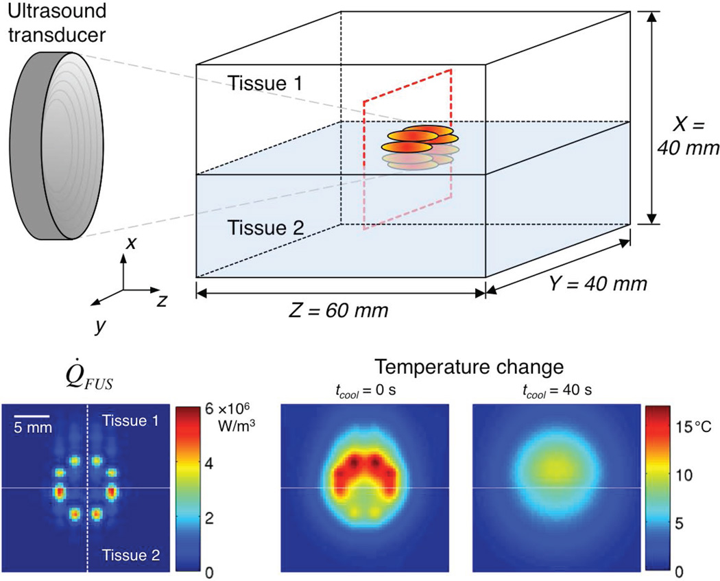
The simulations utilized Pennes BHTE in a two-tissue model (Figure 1). Parameters studied included blood flow, Δt_acq, and MRTI noise. Tissue properties (except blood flow) in Table 1 were from the literature; fat (tissue 1) and muscle (tissue 2) (19–20). Blood flow was modeled with spatially uniform, temporally constant perfusion values, set to 1 kg/m³/s in tissue 1, and adjusted in tissue 2 between 5, 10, and 50 kg/m³/s. The blood specific heat c_bl was equal to the tissue specific heat and T_ar was set equal to the tissues’ initial, uniform value. Adiabatic boundary conditions were applied.

Figure 1.

(Top) Schematic of the two-tissue model used for simulations. The dashed red outline identifies the transverse plane for which the simulated Q̇_FUS pattern (Bottom left) is shown. The horizontal line identifies the tissue interface and the dashed vertical line indicates the position of line plots presented in Figure 2. Representative temperature change data (Bottom middle, t_cool = 0 s; Bottom right, t_cool = 40 s) are also shown, for which the Pennes perfusion parameter values were 1 and 5 kg/m³/s in tissue 1 and tissue 2, respectively.

Table 1.

Tissue properties used in simulations to verify the new technique for quantifying blood flow-related energy losses.

	Units	Tissue 1	Tissue 2
Acoustic Properties
Attenuation coefficient	Np/m	3.3	8.5
Density	kg/m3	911	1090
Speed of sound	m/s	1450	1580
Thermal Properties
Thermal conductivity	W/m/°C	0.21	0.49
Specific heat	J/kg/°C	2348	3421
Thermal diffusivity	mm2/s	0.098	0.131
Blood Flow
Pennes Perfusion	kg/m3/s	1	5, 10, or 50

Heating was simulated using scanned focused ultrasound with eight focal locations, each electronically steered 4.0 mm from the geometric focus. The emitted acoustic power was 40 W. The eight focused ultrasound power deposition patterns (Q̇_FUS) were calculated via the hybrid angular spectrum method (21), superimposed, and averaged to simulate rapid scanning (Figure 1). Heating lasted for 40 s and cooling temperatures were calculated for an additional 40 s. The isotropic grid spacing was 0.4 mm, and the time step was 0.1 s. The finite-difference temperatures were subsampled at Δt_acq values of 1, 2, 4, and 8 s. For a few cases (w = 1, 5 kg/m³/s and Δt_acq = 1, 2, 4, and 8 s), zero-mean Gaussian noise was added to the temperature data (standard deviation (SD) = 0.2 °C).

Q̇_bl values were then estimated for each position during each Δt_acq from the simulated cooling temperature data. To examine the assumption of separability between conduction and blood flow, the values of k∇²T_exp (from the Pennes BHTE simulated experiments) and k∇²T_mod (from the pure conduction model) in Equation 5 were compared after each Δt_acq. The Q̇_bl estimates (Equation 7) were also compared to the values from Equation 2 (using the true perfusion values).

The estimated Q̇_bl and T_acq values were used to estimate a temporally constant w for each location. Finally, those constant w values were used in the Pennes BHTE (with the temperature distribution at the end of heating as the initial condition) to predict temperatures throughout the cooling period.

Simulation results and discussion

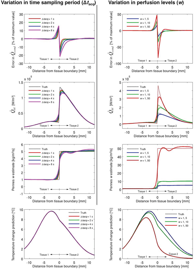
Figure 2 shows how Δt_acq (left column; w = 1, 5 kg/m³/s) and Pennes perfusion parameter (right column; Δt_acq = 4 s) affect the estimation outcomes. Note, the columns’ scales differ, but the blue lines in each column are equivalent, both using w = 1, 5 kg/m³/s and Δt_acq = 4 s.

Figure 2.

Effects of varying Δt_acq (left column; w = 1, 5 kg/m³/s) and Pennes perfusion levels (right column; Δtacq = 4 s) upon outcomes of the simulation study. Errors in Q̇_cond (top row, t_cool = 40 s) evaluate the assumption of conduction and blood flow separability (Equation 5). The true Q̇_bl values (from Equation 2) and estimates (from Equation 7) at t_cool ~ 40 s are seen in the second row. For each position, all Q̇_bl estimates for the 40 s of cooling data are used to calculate constant w estimates (third row), which are then used in the Pennes BHTE to predict cooling temperatures (bottom row, t_cool = 40 s) as a check for self-consistency.

The first row in Figure 2 assesses the conduction and blood flow separability assumption represented by Equation 5 by defining the error in Q̇_cond as a percentage of the maximum k∇²T_exp value, i.e. (k∇²T_mod − k∇²T_exp)/k∇²T_exp,max × 100. This metric preserves comparisons of the errors’ magnitudes at different locations while also providing a sense of their size relative to the overall conduction. It is clear that the separability assumption is least valid near the tissue interface, with error increasing with tissue perfusion differences (Top right). Interface errors also increase with larger Δt_acq (Top left); more importantly, the tissue region with significant Q̇_cond errors widens with increasing Δt_acq (the >1% error region near the interface spans 2.4 and 7.6 mm for Δt_acq of 1 and 8 s, respectively). While the Q̇_cond errors presented in Figure 2 are taken at t_cool = 40 s, results from the rest of the cooling period are very similar (<10% variation).

The second row of Figure 2 shows how errors in the separability assumption affect estimates of Q̇_bl; the magnitude of errors near the interface increases with increasing perfusion differences (second row, right), and the magnitude and spread of errors increase with increasing Δt_acq (second row, left). In essence, the sharp transition in Q̇_bl values at the tissue interface is changed into a smooth transition by the estimation approach. In tissue regions with gradual changes in Q̇_bl, the estimates are excellent, consistently with <1% error. Again, the presented Q̇_bl values at the end of cooling are representative of the entire cooling period, though in general the magnitude of Q̇_bl decreases with time.

The smoothing of Q̇_bl values then blends the tissue discontinuity in the Pennes perfusion parameter w (Figure 2, third row) estimates. Larger Δt_acq widens the region affected by this effect (third row, left). At distances greater than 1.6 mm from the tissue interface, errors in w estimates are consistently less than 5% for all perfusion levels (third row, right).

When w estimates are used in the Pennes BHTE to predict the temperatures from which they were derived (Figure 2, bottom row), the variations caused by different Δt_acq (left) and perfusion levels (right) have minimal effect upon the predicted temperatures, with all errors in predicted temperatures less than 0.1 °C.

Figure 3 demonstrates the effects of MRTI noise. First, the approach clearly requires adequate signal-to-noise ratio (SNR) to produce accurate estimates of w. The white outline in the leftmost image identifies the region with > 5 °C temperature rise in the noiseless data. Mean estimates of perfusion in this region approach the true values (Table 2). Outside this region, MRTI noise confounds the results. Second, the smoothing effect seen at perfusion discontinuities now beneficially reduces variation in w estimates caused by noise. Longer Δt_acq therefore produces cleaner estimates of the perfusion profile. Table 2 shows this trend quantitatively, where the SD of w decreases with increasing Δt_acq.

Figure 3.

Effects of Gaussian noise in the simulated temperature data (SD = 0.2 °C) upon estimates of the Pennes perfusion parameter w for different Δt_acq. The white outline on the true w image (left) identifies locations that had a temperature rise of at least 5 °C at the beginning of cooling.

Table 2.

Mean ± SD of Pennes perfusion parameter w estimates from noisy simulations as a function of Δt_acq for all locations experiencing > 5 °C temperature rise (white outline in leftmost image of Figure 3). The noise SD was 0.2 °C and the actual, uniform w values were 1 kg/m³/s for tissue 1 and 5 kg/m³/s for tissue 2.

Δtacq s	w: tissue 1 kg/m3/s	w: tissue 2 kg/m3/s
1	1.0 ± 3.3	4.5 ± 5.3
2	1.2 ± 2.5	4.6 ± 3.9
4	1.2 ± 1.9	4.8 ± 2.8
8	1.2 ± 1.3	4.6 ± 2.0

In conclusion, the approach introduces a finite-difference conduction model based on separability of conduction and blood flow effects during Δt_acq. Simulations demonstrate that this approach smooths sharp transitions in blood flow, with a broadening of the affected region for longer Δt_acq. The smoothing effect reduces errors introduced by MRTI noise. A strong temperature signal is necessary for obtaining meaningful results with this approach. In regions without sharp discontinuities in blood flow, the approach generates correct Q̇_bl and w estimates with accurate temperature predictions.

Experimental study

Experimental methods

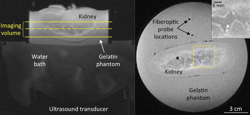
The experimental study was performed in an ex vivo perfused porcine kidney (Figure 4). Following excision and cannulation of the renal artery, the kidney was flushed with a heparin and saline solution (38). The kidney was secured in a gelatin phantom to provide a region for referenceless temperature reconstruction (39). In the coronal T1-weighted magnitude image of Figure 4, acquired during 40 ml/min flow with no heating, the yellow box identifies the region of interest (ROI) used for presenting the experimental results. This ROI has been magnified in the top right inset of Figure 4 where high flow locations can be identified by their bright intensity.

Figure 4.

Experimental setup for MRgFUS heating of ex vivo perfused porcine kidney. In the axial image at left, the temperature imaging volume lies between the yellow solid lines. The dashed yellow line identifies the position of the coronal T1-weighted magnitude image at right. The blue circle indicates the focused ultrasound heating region for location 1 and the yellow box indicates the inset region of interest (top right) where bright spots identify locations of high flow. This inset corresponds to the ROI for data presented in Figures 5–7,10. For heating at location 2, the blue circle and yellow box are shifted and centered upon the black asterisk.

Heating was achieved by electronically steering a 256-element phased-array ultrasound transducer (Imasonics, Besancon, France and Image Guided Therapy, Pessac, France) rapidly in an 8-mm radius circle (blue circle, Figure 4) for 120 s at 90 acoustic watts. The kidney was perfused with a heparin-H₂O solution at fixed flow rates (0, 20, and 40 ml/min) (40). To obtain a high, consistent temperature distribution at the start of cooling, flow was kept at zero during heating and initiated at the start of the cooling period. Two heating scans were performed at each of the three flow rates in two different locations yielding twelve data sets. For the second heating location, the blue circle for focused ultrasound heating and yellow box for results was shifted and centered on the asterisk in Figure 4.

MR data were acquired in 10 coronal slices with a 3T Siemens Trio MRI (3D segmented-EPI, TR/TE = 30/11 ms, FOV = 192×156×30 mm³, FA = 15°, 694 Hz/pixel, EPI factor = 9, 2×2×3 mm³, Δt_acq = 3.3 s) using a custom-built, single-channel loop coil. Temperatures were reconstructed via the proton resonance frequency method (41–42) with a 2D referenceless reconstruction technique using a fifth-order polynomial (39), and zero filled interpolated to 0.5-mm isotropic spacing (43–44). Kidney properties were obtained via invasive probe measurements (KD2 Pro, Decagon Devices, Pullman, WA) and the displaced-water technique following the experiment.

The temperature data were utilized to quantify Q̇_bl using Equation 7 for each voxel and acquisition interval. Conduction model calculations used a finite-difference spacing that matched the zero-filled interpolated voxel size (0.5 mm-isotropic) and a time step of 0.1 s. Adiabatic boundary conditions were assumed.

Over the course of the experiment, fiberoptic probes in the gelatin phantom indicated that the background tissue temperature increased from 21.8 to 27.6 °C. Since the background tissue temperature is used as a reference baseline for MRTI and the perfusate temperature (23.0 °C) was constant throughout the experiment, T_ar, defined as the difference between the perfusate and the background tissue temperatures, changed slowly from 1.2 to −4.6 °C during the experiment; however, for the few minutes needed to acquire MRTI data from each individual heating scan, T_ar was assumed to be constant. A minimum of 10 minutes cooling was implemented between experiments to allow for thermal equilibrium before data acquisition.

Two approaches were implemented for determining the Pennes perfusion parameter w. First (spatially varying w), 60 s of Q̇_bl and T_ave data were used to optimize for a temporally constant w in each voxel. The optimization routine (MATLAB function fminsearch) updated w to minimize the least-squares error between experimentally determined Q̇_bl values (Equation 7) and those predicted by Equation 2. Q̇_bl values from the first two MRTI acquisitions of the cooling period were not used to avoid non-steady state perfusate flows. Therefore, Q̇_bl and T_ave values from t_cool = 10.7–69.6 s were used to find w on a voxel-by-voxel basis.

Second (spatially uniform w), all of the Q̇_bl and T_ave values in a 2×2×2 cm³ region (centered in the yellow box of Figure 4) over the time period from t_cool = 10.7–69.6 s were used to optimize for a single average w value in space and time. To determine whether those MRTI-based w values were of appropriate magnitude, simplified uniform perfusion values were also calculated according to

$$\mathit{\text{Perfusion}}\left(\frac{kg}{m^3·s}\right)=\frac{\mathit{\text{Flow rate}}(ml/s)*\mathit{\text{Perfusate density}}(kg/m^3)}{\mathit{\text{kidney volume}}(ml)}.$$ (8)

Finally, the predictive ability of w values obtained in this study was tested in simulations using the Pennes BHTE. Temperatures were predicted for 68.0 s of cooling using both spatially varying and spatially uniform w values. Experimental temperatures just prior to cooling were used as the initial condition with adiabatic boundary conditions. Maximum errors and root-mean-squared errors (RMSE) were calculated for the inset ROI of Figure 4.

Experimental results and discussion

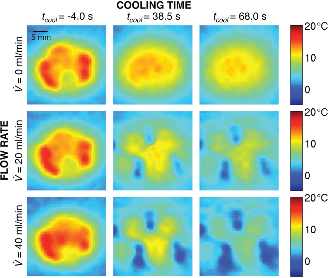
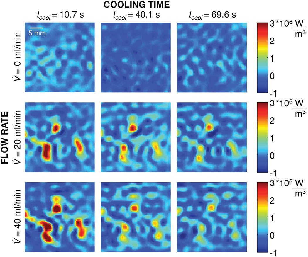
Representative temperature change profiles at different times and flow rates are shown in Figure 5. The initial temperature distributions (left column) are similar for all flow conditions as expected (mean temperature differences < 0.2 °C), because the perfusate flow was always off during heating and the applied power was equivalent. Later in the cooling period (center and right columns), temperature profiles at different flow rates diverge, with regions of greatest cooling (blue) corresponding to high flow locations (Figure 4, inset).

Figure 5.

Experimental MR temperature changes at the end of heating (left column), 38.5 s (center column) and 68.0 s (right column) into the cooling period for flow rates of 0 ml/min (top row), 20 ml/min (middle row), and 40 (bottom row) ml/min.

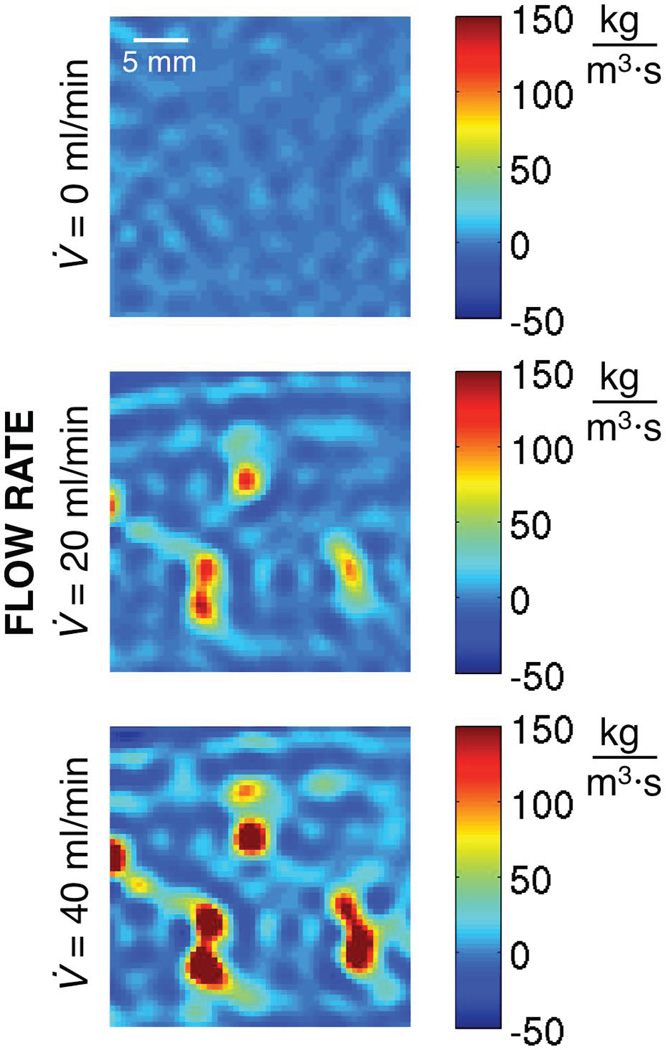
Figure 6 shows the values of Q̇_bl corresponding to the temperature profiles of Figure 5 (the left column has been delayed several MR acquisitions to ensure a steady perfusate flow). For the 0 ml/min case (top row), there are no energy losses caused by flow and, as expected, the calculated Q̇_bl values are approximately zero; nonzero Q̇_bl values represent variations caused by MRTI noise and/or errors in the approach’s approximations. For 20 ml/min (middle row) and 40 ml/min (bottom row), the locations of greatest Q̇_bl (red) correspond to the locations of greatest cooling (blue) in Figure 5. As time progresses, the initially large Q̇_bl values decrease because energy is continually being drawn away by the perfusate. All blood flow related-energy losses, both convective losses to large vessels and Pennes sink-like perfusion losses, are accounted for in Q̇_bl, with no indication of the specific mechanism.

Figure 6.

Spatially varying, dynamic values of perfusion-related energy losses (Q̇_bl) at different times in the cooling period for three different flow rates.

Q̇_bl is a function of both the flow magnitude and the amount of thermal energy in the tissue. Early in cooling, Q̇_bl is larger for the 40 ml/min case than the 20 ml/min case, because the flow rate is greater and the thermal energy in the tissue is approximately the same at this time. Later, the Q̇_bl values are greater for the 20 ml/min case than the 40 ml/min case. It appears that the tissue quickly reaches thermal equilibrium with the perfusate in high flow regions at 40 ml/min, so there is limited residual energy to be drawn away by the perfusate at the later times.

Once the 3D distributions of Q̇_bl are determined, they can be used to evaluate the Pennes BHTE. While the empirically derived Pennes perfusion parameter is only equal to the true capillary blood perfusion in limited situations (25), reported capillary blood perfusion values can help identify appropriate magnitudes of w. For reference, average fat and resting muscle perfusions are 0.55 and 0.65 kg/m³/s, respectively, brain perfusion is 9.3 kg/m³/s, liver is 15 kg/m³/s, and kidney is 69 kg/m³/s (20). If large vessels traverse the MRgFUS heated region, much larger local perfusion values could be calculated since the Pennes model does not distinguish between convective and perfusion effects. In such cases, w is only an empirical parameter accounting for blood flow-related energy losses.

Spatially varying estimates of w (assumed constant in time) are presented in Figure 7. For the no-flow case (top), w values have a mean of −0.7 kg/m³/s and range from −13.7 to 15.1 kg/m³/s. Ideally, all of these values should be zero. Despite the optimization in time, MRTI noise (SD = 0.2 °C for these data) is still introducing variation in w estimates. For flow situations (middle and bottom), values of w increase with increasing flow rate and the largest w values correspond to high flow locations identified in Figure 4.

Figure 7.

Spatially varying Pennes perfusion parameter w optimized in each voxel for a single constant value over ~60 s of cooling for three different flow rates.

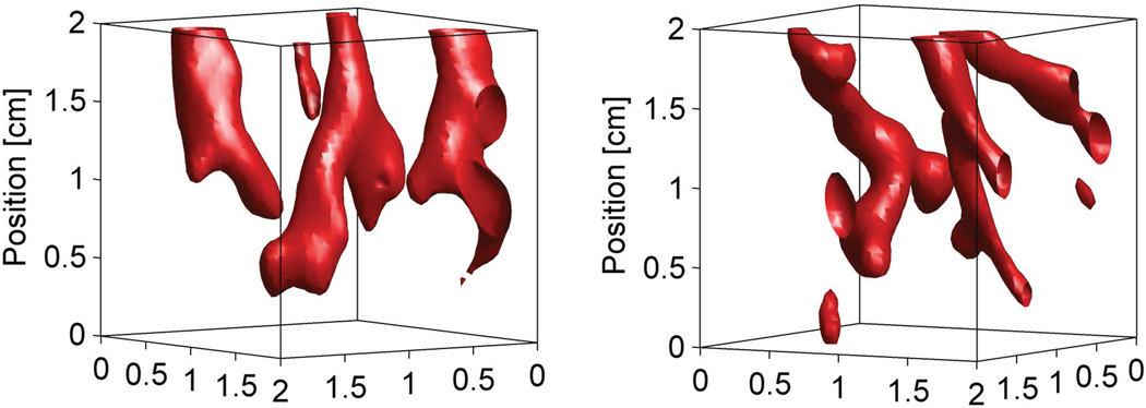
Figures 5–7 show only a single, representative 2D slice from three data sets. Figure 8 highlights the three-dimensional nature of this study, showing projections of the spatially varying w values (flow rate = 40 ml/min) that are greater than 125 kg/m³/s in a 2×2×2 cm³ region centered on the heated volume. The two projections, from different heating locations, approximately trace the discrete kidney vasculature.

Figure 8.

Three-dimensional projections of spatially varying Pennes perfusion parameter w values greater than 125 kg/m³/s in an 8 (2×2×2) cm³ region centered on the heated volume. The projections were obtained from data sets with a flow rate of 40 ml/min at different locations of the kidney. The ultrasound transducer is positioned below the projected images.

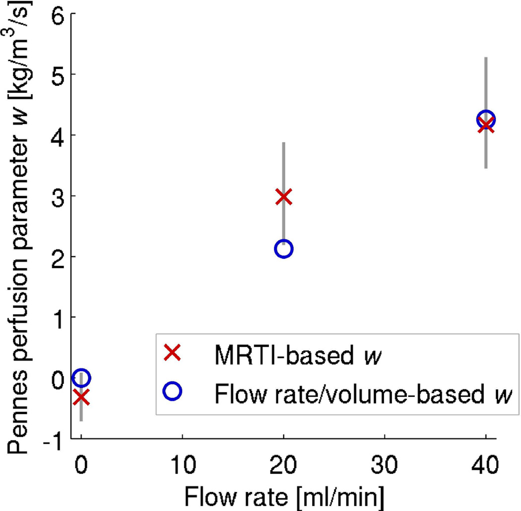
Figure 9 shows results from all twelve data sets using a spatially uniform w. Red × markers indicate the average of w estimates at each flow rate (n=4) with vertical bars identifying the range of measured values. The average values increase as anticipated, −0.3, 3.0, and 4.2 kg/m³/s for flow rates of 0, 20, and 40 ml/min, respectively. These are a fraction of published values (69 kg/m³/s) for in vivo kidney (20), because the experimental flow rates are much lower than those experienced in vivo (estimated at ~700 ml/min using Equation 8). Attempts to perfuse the ex vivo kidney at in vivo flow rates caused cannulation sutures to fail. However, comparison with the simplified uniform perfusion values (blue circle markers) calculated from Equation 8 for the ex vivo experimental flow rates shows that the MRTI-based w values are of an appropriate magnitude. One might expect that experimental values would increase linearly with flow rate, but this was not observed in our experiments, potentially due to the limited sample size, residual noise effects, or non-uniform increases of perfusate flow in the kidney as the flow rate was increased.

Figure 9.

Average values of the spatially uniform Pennes perfusion parameter w based on MRTI data (n=4 for each flow rate) are represented by red × markers. Vertical lines indicate the full range of those estimates. Blue circle markers denote calculations of uniform perfusion based upon the flow rate and kidney volume.

Considering the four 0 ml/min data sets where estimates should be zero, MRTI-based values of w range from −0.7 to 0.1 kg/m³/s. These errors are approximately the range of perfusion values for fat and resting muscle and suggest that this technique may need to be improved to have sufficient sensitivity for measurements in those and other low perfusion tissues, unless improvements in MRTI SNR are made. However, such small perfusion values would have little impact on MRgFUS temperatures and may not be critical for pretreatment planning purposes.

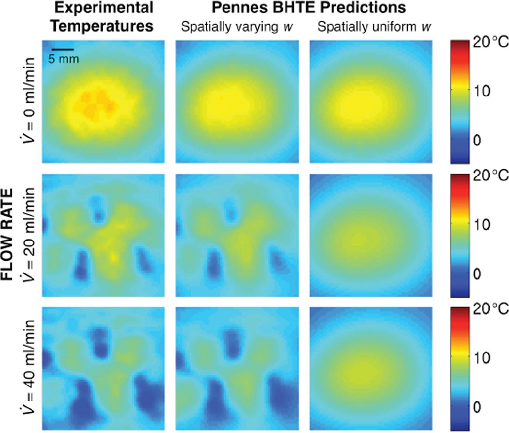
Without independent measurements of perfusion or blood flow, testing the ability of w estimates to predict temperature changes is an appropriate method for assessing their magnitude. The left column of Figure 10 repeats the experimental temperatures at t_cool = 68.0 s from Figure 5. Temperature predictions from simulations of the Pennes BHTE using either spatially varying w (center) or spatially uniform w (right) are shown in the adjacent columns. Maximum temperature errors and RMSE for the Pennes BHTE temperature predictions are found in Table 3. By using spatially varying instead of spatially uniform w, maximum errors in temperature prediction are reduced by an average of 27% for the no-flow case, 72% for the 20 ml/min case, and by 73% for the 40 ml/min case. RMSE values are reduced on average by 2%, 67%, and 79% for the 0, 20, and 40 ml/min cases, respectively. Such predictions help assess the self-consistency of the model being evaluated.

Figure 10.

Experimental temperatures after 68.0 s of cooling (left column) are compared with temperature predictions from simulations of Pennes BHTE with either spatially varying w values (center column) or spatially uniform w values (right column).

Table 3.

Maximum errors and RMSE for temperature predictions from Pennes BHTE.

	Pennes BHTE predictions
Flow rate (ml/min)	Spatially varying w		Spatially uniform w
	Max error (°C)	RMSE (°C)	Max error (°C)	RMSE (°C)
0*	1.4	0.6	1.7	0.7
0	1.0	0.3	1.1	0.4
0	2.6	0.8	4.0	0.8
0	1.7	0.6	3.2	0.5
20*	1.5	0.5	7.0	1.8
20	4.0	0.6	8.3	2.0
20	2.5	0.8	9.7	2.0
20	1.7	0.5	9.4	2.0
40*	3.1	0.6	8.9	2.7
40	3.4	0.7	9.3	3.0
40	1.9	0.4	9.3	2.6
40	1.9	0.7	11.6	3.2

^*indicates data sets corresponding to Figure 10 results.

The Pennes BHTE using spatially uniform values for w is least accurate near large blood vessels (25,31,33,45–47). This study supports that conclusion, since temperature predictions using a spatially uniform w (right column of Figure 10) are especially poor in the high flow regions identified in Figure 4. However, most methods for experimentally estimating w will only identify a single uniform value (12–13,48–49), and property tables only provide average values (17–18,20). The inclusion of discrete vasculature in thermal modeling significantly improves temperature prediction, but requires a priori knowledge of the vessel network and increases the complexity of thermal models (50–52).

The accurate predictive power of the spatially varying Pennes model used in this study suggests that the Pennes BHTE, while not ideal, may be useful and appropriate for some cases of vascularized tissues if w can be evaluated and implemented on a voxel-by-voxel basis instead of uniformly. Errors in the temperature predictions are still greatest near large vessels, but are significantly smaller than those made using spatially uniform w values. Thus, while the Pennes model may not accurately represent the details of convective heat transfer, the self-consistency demonstrated in temperature predictions suggests that it can at least coarsely reflect the nature of thermal energy losses to large vessels. For considerations of pretreatment planning in vascularized tissues like this kidney model, the spatially varying Pennes model is superior to the spatially uniform Pennes model. The residual RMSE seen in Table 3 suggest that further improvements are possible. Future models of increased complexity should provide better results. However, residual RMSE may in part be attributed to sources beyond model insufficiencies, such as MRTI drift or noise and the variability of equipment or experimental execution.

The technique used in this study for quantifying Q̇_bl can also be applied using MRTI heating data, but introduces an additional source of uncertainty by requiring knowledge of Q̇_FUS in Equation 1. Utilizing heating data would be particularly helpful for the more realistic case of continuous blood flow through the heating and cooling periods. Clinically, it is not practical to restrict blood flow during heating as was artificially done in the presented experiment, though some pre-clinical studies have shown it is possible (53). Blood flow during the heating period would lower the magnitude of the temperature rise and create large local temperature gradients. If Q̇_FUS is known, the additional heating data could help offset these adverse effects by providing more information for Q̇_bl quantification and model evaluations.

In equating the two conduction terms of Equation 5, this approach assumes that blood flow and conduction effects are separable over short time intervals (Δt_acq). In practice, where the assumption is least valid (at blood flow discontinuities), the finite-difference model smooths sharp transitions and introduces a blending effect in Q̇_bl and w values. This effect is seen in simulations at the interface between tissues (Figure 2) and is likely present on the edges of the high flow locations in the kidney. With very localized blood flow discontinuities such as those at high flow vessels, the smoothing effect may prevent this approach from capturing the true magnitude of Q̇_bl, most likely resulting in underestimation of Q̇_bl within the vessel. Improving the temporal resolution of MRTI will mitigate such errors by minimizing the time for which the finite-difference model approximation is applied, but will also reduce the SNR of MRTI data and the ability of the model to smooth errors introduced by MRTI noise.

The accuracy of results depends in part upon the accuracy of the approximations and a priori knowledge required by the technique. In this paper, we have assumed uniform, constant tissue thermal properties. Errors in the assumed local tissue property values will be reflected in the estimated Q̇_bl values, as the technique will compensate for errors by adjusting Q̇_bl. This is not a limitation of the technique itself, since if the thermal properties were known, they could be implemented in the technique.

In spite of the challenges described above, the self-consistency demonstrated by this approach when implementing the relatively simple, spatially variable Pennes BHTE is encouraging for its use in evaluating Pennes and other BHTE models. Of note, another technique was recently proposed for using the Pennes BHTE to simultaneously reconstruct the distribution of tissue thermal properties, blood flow, and metabolic heat generation from simulated heating data caused by transmit RF coils (54). That technique was also shown to be least accurate at interfaces between tissues and at flow discontinuities.

Currently, this approach is only clinically applicable in retrospective studies, because the tissue heating required to obtain Q̇_bl for biothermal model evaluation is not reasonable in the pretreatment setting. To fully configure these techniques for clinical use, an independent and quantitative measure of blood flow is essential, e.g. arterial spin labeling or dynamic contrast enhanced imaging (55–56). For pretreatment planning, such quantitative blood flow measurements will need to be converted through the biothermal model parameters to the blood flow-related energy losses. Our approach is one possible method for calibrating that conversion. Once this goal is accomplished, biothermal models for treatment planning will have the ability to accurately predict temperature distributions, dose profiles, and treatment outcomes before the thermal therapy begins.

Conclusion

The novel 3D MRTI-based approach presented in this study for quantifying blood flow-related energy losses and evaluating the Pennes BHTE is a step forward from past validation efforts, because the extensive 3D MRTI data allow evaluation with greater spatial and temporal sensitivity. The finite-difference model implemented in the approach blends sharp transitions in blood flow and mitigates noise effects. Estimates of spatially varying Pennes perfusion parameter w values yielded significantly more accurate temperature predictions than the traditionally implemented spatially uniform w. This approach has promise in both quantifying the role of blood flow in treatments and in the comprehensive evaluation of biothermal models used in MRgFUS thermal therapies.

Abbreviations

BHTE

bioheat transfer equation

MRTI

magnetic resonance temperature imaging

MRgFUS

magnetic resonance-guided focused ultrasound

Q̇_bl

blood flow-related energy losses [W/m³]

Q̇_FUS

focused ultrasound power deposition [W/m³]

ROI

region of interest

RMSE

root-mean-squared error

SD

standard deviation

SNR

signal-to-noise ratio

Δt_acq

MRTI acquisition time interval [s]

w

Pennes perfusion parameter [kg/m³/s]

References

- 1.Chen L, ter Haar G, Hill CR, Dworkin M, Carnochan P, Young H, Bensted JPM. Effect of blood perfusion on the ablation of liver parenchyma with high-intensity focused ultrasound. Phys. Med. Biol. 1993;38(11):1661–1673. doi: 10.1088/0031-9155/38/11/011. [DOI] [PubMed] [Google Scholar]
- 2.McDannold N, Tempany CM, Fennessy FM, So MJ, Rybicki FJ, Stewart EA, Jolesz FA, Hynynen K. Uterine leiomyomas: MR imaging–based thermometry and thermal dosimetry during focused ultrasound thermal ablation. Radiology. 2006;240(1):263–272. doi: 10.1148/radiol.2401050717. [DOI] [PMC free article] [PubMed] [Google Scholar]
- 3.Lenard ZM, McDannold NJ, Fennessy FM, Stewart EA, Jolesz FA, Hynynen K, Tempany CM. Uterine Leiomyomas: MR imaging-guided focused ultrasound surgery-imaging predictors of success. Radiology. 2008;249(1):187–194. doi: 10.1148/radiol.2491071600. [DOI] [PMC free article] [PubMed] [Google Scholar]
- 4.Zhang L, Zhu H, Jin C, Zhou K, Li K, Su H, Chen W, Bai J, Wang Z. High-intensity focused ultrasound (HIFU): effective and safe therapy for hepatocellular carcinoma adjacent to major hepatic veins. Eur. Radiol. 2009;19(2):437–445. doi: 10.1007/s00330-008-1137-0. [DOI] [PubMed] [Google Scholar]
- 5.Billard BE, Hynynen K, Roemer RB. Effects of physical parameters on high temperature ultrasound hyperthermia. Ultrasound Med. Biol. 1990;16(4):409–420. doi: 10.1016/0301-5629(90)90070-s. [DOI] [PubMed] [Google Scholar]
- 6.Albrecht D, Germer CT, Isbert C, Ritz JP, Roggan A, Müller G, Buhr HJ. Interstitial laser coagulation: evaluation of the effect of normal liver blood perfusion and the application mode on lesion size. Laser Surg. Med. 1998;23(1):40–47. doi: 10.1002/(sici)1096-9101(1998)23:1<40::aid-lsm6>3.0.co;2-w. [DOI] [PubMed] [Google Scholar]
- 7.Goldberg SN, Hahn PF, Tanabe KK, Mueller PR, Schima W, Athanasoulis CA, Compton CC, Solbiati L, Gazelle GS. Percutaneous radiofrequency tissue ablation: does perfusion-mediated tissue cooling limit coagulation necrosis? J. Vasc. Interv. Radiol. 1998;9(1):101–111. doi: 10.1016/s1051-0443(98)70491-9. [DOI] [PubMed] [Google Scholar]
- 8.Shih TC, Liu HL, Horng ATL. Cooling effect of thermally significant blood vessels in perfused tumor tissue during thermal therapy. Int. Commun. Heat Mass. 2006;33(2):135–141. [Google Scholar]
- 9.Payne A, Vyas U, Todd N, de Bever J, Christensen DA, Parker DL. The effect of electronically steering a phased array ultrasound transducer on near-field tissue heating. Med. Phys. 2011;38(9):4971–4981. doi: 10.1118/1.3618729. [DOI] [PMC free article] [PubMed] [Google Scholar]
- 10.Dewhirst MW, Gibbs FA, Jr, Roemer RB, Samulski TV. Hyperthermia. In: Gunderson LL, Tepper JE, editors. Clinical Radiation Oncology. New York: Churchill Livingstone; 2000. pp. 256–282. [Google Scholar]
- 11.de Bever J, Todd N, Payne A, Christensen DA, Roemer RB. Adaptive model-predictive controller for magnetic resonance guided focused ultrasound therapy. Int. J. Hyperthermia. 2014;30(7):456–470. doi: 10.3109/02656736.2014.968223. [DOI] [PubMed] [Google Scholar]
- 12.Cheng HLM, Plewes DB. Tissue thermal conductivity by magnetic resonance thermometry and focused ultrasound heating. J. Magn. Reson. Imaging. 2002;16(5):598–609. doi: 10.1002/jmri.10199. [DOI] [PubMed] [Google Scholar]
- 13.Dragonu I, de Oliveira PL, Laurent C, Mougenot C, Grenier N, Moonen CT, Quesson B. Non-invasive determination of tissue thermal parameters from high intensity focused ultrasound treatment monitored by volumetric MRI thermometry. NMR Biomed. 2009;22(8):843–851. doi: 10.1002/nbm.1397. [DOI] [PubMed] [Google Scholar]
- 14.Dillon CR, Vyas U, Payne A, Christensen DA, Roemer RB. An analytical solution for improved HIFU SAR estimation. Phys. Med. Biol. 2012;57(14):4527–4544. doi: 10.1088/0031-9155/57/14/4527. [DOI] [PMC free article] [PubMed] [Google Scholar]
- 15.Dillon CR, Payne A, Christensen DA, Roemer RB. The accuracy and precision of two non-invasive, magnetic resonance-guided focused ultrasound-based thermal diffusivity estimation methods. Int. J. Hyperthermia. 2014;30(6):362–371. doi: 10.3109/02656736.2014.945497. [DOI] [PMC free article] [PubMed] [Google Scholar]
- 16.Zhang J, Fischer J, Warner L, Oto A, Hor PH, Muthupillai R. Noninvasive, in vivo determination of uterine fibroid thermal conductivity in MRI-guided high intensity focused ultrasound therapy. J. Magn. Res. Imaging. 2014 doi: 10.1002/jmri.24724. [DOI] [PubMed] [Google Scholar]
- 17.Duck FA. Physical properties of tissues: a comprehensive reference book. Academic Press; 1990. [Google Scholar]
- 18.Holmes KR. Thermal properties. [Accessed September 2014];1999 http://users.ece.utexas.edu/~valvano/research/Thermal.pdf. [Google Scholar]
- 19.International Commission on Radiation Units and Measurements. Bethesda, MD: ICRU Publications; 1998. ICRU report 61: tissue substitutes, phantoms and computational modelling in medical ultrasound. [Google Scholar]
- 20.Hasgall PA, Neufeld E, Gosselin MC, Klingenböck A, Kuster N. IT’IS database for thermal and electromagnetic parameters of biological tissues. Version 2.5. 2014 www.itis.ethz.ch/database. [Google Scholar]
- 21.Vyas U, Christensen DA. Ultrasound beam simulations in inhomogeneous tissue geometries using the hybrid angular spectrum method. IEEE Trans. Ultrason. Ferroelectr. Freq. Control. 2012;59(6):1093–1100. doi: 10.1109/tuffc.2012.2300. [DOI] [PubMed] [Google Scholar]
- 22.Pulkkinen A, Werner B, Martin E, Hynynen K. Numerical simulations of clinical focused ultrasound functional neurosurgery. Phys. Med. Biol. 2014;59(7):1679–1700. doi: 10.1088/0031-9155/59/7/1679. [DOI] [PMC free article] [PubMed] [Google Scholar]
- 23.Pennes HH. Analysis of tissue and arterial blood temperatures in the resting human forearm. J. Appl. Physiol. 1948;1(2):93–122. doi: 10.1152/jappl.1948.1.2.93. [DOI] [PubMed] [Google Scholar]
- 24.Chen MM, Holmes KR. Microvascular contributions to tissue heat transfer. Ann. NY Acad. Sci. 1980;335(1):137–150. doi: 10.1111/j.1749-6632.1980.tb50742.x. [DOI] [PubMed] [Google Scholar]
- 25.Roemer RB, Dutton AW. A generic tissue convective energy balance equation: Part I-theory and derivation. J. Biomech. Eng. 1998;120(3):395–404. doi: 10.1115/1.2798007. [DOI] [PubMed] [Google Scholar]
- 26.Weinbaum S, Jiji LM. A new simplified bioheat equation for the effect of blood flow on local average tissue temperature. J. Biomech. Eng. 1985;107(2):131–139. doi: 10.1115/1.3138533. [DOI] [PubMed] [Google Scholar]
- 27.Weinbaum S, Xu LX, Zhu L, Ekpene A. A new fundamental bioheat equation for muscle tissue: Part I-perfusion term. J. Biomech. Eng. 1997;119(3):278–288. doi: 10.1115/1.2796092. [DOI] [PubMed] [Google Scholar]
- 28.Wissler EH. Pennes’ 1948 paper revisited. J. Appl. Physiol. 1998;85(1):35–41. doi: 10.1152/jappl.1998.85.1.35. [DOI] [PubMed] [Google Scholar]
- 29.Mitchell JW, Galvez TL, Hengle J, Myers GE, Siebecker KL. Thermal response of human legs during cooling. J. Appl. Physiol. 1970;29(6):859–865. doi: 10.1152/jappl.1970.29.6.859. [DOI] [PubMed] [Google Scholar]
- 30.Sekins KM, Lehmann JF, Esselman P, Dundore D, Emery AF, Delateur BJ, Nelp WB. Local muscle blood flow and temperature responses to 915MHz diathermy as simultaneously measured and numerically predicted. Arch. Phys. Med. Rehabil. 1984;65(1):1–7. [PubMed] [Google Scholar]
- 31.Moros EG, Dutton AW, Roemer RB, Burton M, Hynynen K. Experimental evaluation of two simple thermal models using hyperthermia in muscle in vivo. Int. J. Hyperthermia. 1993;9(4):581–598. doi: 10.3109/02656739309005054. [DOI] [PubMed] [Google Scholar]
- 32.Crezee J, Lagendijk JW. Experimental verification of bioheat transfer theories: measurement of temperature profiles around large artificial vessels in perfused tissue. Phys. Med. Biol. 1990;35(7):905–923. doi: 10.1088/0031-9155/35/7/007. [DOI] [PubMed] [Google Scholar]
- 33.Crezee J, Mooibroek J, Lagendijk JJW, Van Leeuwen GMJ. The theoretical and experimental evaluation of the heat balance in perfused tissue. Phys. Med. Biol. 1994;39(5):813–832. doi: 10.1088/0031-9155/39/5/003. [DOI] [PubMed] [Google Scholar]
- 34.Kolios MC, Worthington AE, Sherar MD, Hunt JW. Experimental evaluation of two simple thermal models using transient temperature analysis. Phys. Med. Biol. 1998;43(11):3325–3340. doi: 10.1088/0031-9155/43/11/011. [DOI] [PubMed] [Google Scholar]
- 35.Dillon CR. PhD Dissertation. University of Utah; 2014. Identifying parameters from the bioheat transfer equation using magnetic resonance-guided focused ultrasound. [Google Scholar]
- 36.Carluccio G, Oh S, Collins C. Ultra-fast calculation of SAR-induced termperature increase; Proc. 19th Ann. Mtg. ISMRM; 2011. p. 1844. [Google Scholar]
- 37.Carluccio G, Erricolo D, Oh S, Collins CM. An approach to rapid calculation of temperature change in tissue using spatial filters to approximate effects of thermal conduction. IEEE T. Biomed. Eng. 2013;60(6):1735–1741. doi: 10.1109/TBME.2013.2241764. [DOI] [PMC free article] [PubMed] [Google Scholar]
- 38.Holmes KR, Ryan W, Weinstein P, Chen MM. A fixation technique for organs to be used as perfused tissue phantoms in bioheat transfer studies. ASME Adv. Bioeng. 1948:9–10. [Google Scholar]
- 39.Rieke V, Vigen KK, Sommer G, Daniel BL, Pauly JM, Butts K. Referenceless PRF shift thermometry. Magn. Reson. Med. 2004;51(6):1223–1231. doi: 10.1002/mrm.20090. [DOI] [PubMed] [Google Scholar]
- 40.Payne A, Goodrich KC, Kholmovski EG, Roemer RB, Parker DL. Isolated kidney phantom for development of biothermal vascular models with application to high intensity focused ultrasound therapy. Med. Phys. 2008;35(10):4426–4434. doi: 10.1118/1.2975226. [DOI] [PubMed] [Google Scholar]
- 41.De Poorter JD, De Wagter C, De Deene Y, Thomsen C, Stahlberg F, Achten E. Noninvasive MRI thermometry with the proton resonance frequency (PRF) method: in vivo results in human muscle. Magn. Reson. Med. 1995;33(1):74–81. doi: 10.1002/mrm.1910330111. [DOI] [PubMed] [Google Scholar]
- 42.Ishihara Y, Calderon A, Watanabe H, Okamoto K, Suzuki Y, Kuroda K, Suzuki Y. A precise and fast temperature mapping using water proton chemical shift. Magn. Reson. Med. 1995;34(6):814–823. doi: 10.1002/mrm.1910340606. [DOI] [PubMed] [Google Scholar]
- 43.Todd N, Vyas U, de Bever J, Payne A, Parker DL. The effects of spatial sampling choices on MR temperature measurements. Magn. Reson. Med. 2011;65(2):515–521. doi: 10.1002/mrm.22636. [DOI] [PMC free article] [PubMed] [Google Scholar]
- 44.Dillon CR, Todd N, Payne A, Parker DL, Christensen DA, Roemer RB. Effects of MRTI sampling characteristics on estimation of HIFU SAR and tissue thermal diffusivity. Phys. Med. Biol. 2013;58(20):7291–7307. doi: 10.1088/0031-9155/58/20/7291. [DOI] [PMC free article] [PubMed] [Google Scholar]
- 45.Kolios MC, Sherar MD, Hunt JW. Blood flow cooling and ultrasonic lesion formation. Med. Phys. 1996;23(7):1287–1298. doi: 10.1118/1.597694. [DOI] [PubMed] [Google Scholar]
- 46.Kolios MC, Worthington AE, Holdsworth DW, Sherar MD, Hunt JW. An investigation of the flow dependence of temperature gradients near large vessels during steady state and transient tissue heating. Phys. Med. Biol. 1999;44(6):1479–1497. doi: 10.1088/0031-9155/44/6/304. [DOI] [PubMed] [Google Scholar]
- 47.Huang HW, Shih TC, Liauh CT. Predicting effects of blood flow rate and size of vessels in a vasculature on hyperthermia treatments using computer simulation. Biomed. Eng. Online. 2010;9:18. doi: 10.1186/1475-925X-9-18. [DOI] [PMC free article] [PubMed] [Google Scholar]
- 48.Roemer RB, Fletcher AM, Cetas TC. Obtaining local SAR and blood perfusion data from temperature measurements; steady state and transient techniques compared. Int. J. Radiat. Oncol. Biol. Phys. 1985;11(8):1539–1550. doi: 10.1016/0360-3016(85)90343-8. [DOI] [PubMed] [Google Scholar]
- 49.Kress R, Roemer R. A comparative analysis of thermal blood perfusion measurement techniques. J. Biomech. Eng. 1987;109(3):218–225. doi: 10.1115/1.3138672. [DOI] [PubMed] [Google Scholar]
- 50.Rawnsley RJ, Roemer RB, Dutton AW. The simulation of discrete vessel effects in experimental hyperthermia. J. Biomech. Eng. 1994;116(3):256–262. doi: 10.1115/1.2895728. [DOI] [PubMed] [Google Scholar]
- 51.Kotte A, van Leeuwen G, de Bree J, van der Koijk J, Crezee H, Lagendijk J. A description of discrete vessel segments in thermal modelling of tissues. Phys. Med Biol. 1996;41(5):865–884. doi: 10.1088/0031-9155/41/5/004. [DOI] [PubMed] [Google Scholar]
- 52.Deng ZS, Liu J. Numerical study of the effects of large blood vessels on three-dimensional tissue temperature profiles during cryosurgery. Numer. Heat Tr. A-Appl. 2006;49(1):47–67. [Google Scholar]
- 53.Cornelis F, Grenier N, Moonen CT, Quesson B. In vivo characterization of tissue thermal properties of the kidney during local hyperthermia induced by MR-guided high-intensity focused ultrasound. NMR Biomed. 2011;24:799–806. doi: 10.1002/nbm.1624. [DOI] [PubMed] [Google Scholar]
- 54.Alon L, Collins C, Carluccio G, Novikov D, Zhu Y, Sodickson D. Tissue thermal property tomography. Proc. Intl. Soc. Mag. Reson. Med. 2013;21:2519. [Google Scholar]
- 55.Knutsson L, van Westen D, Petersen ET, Bloch KM, Holtas S, Stahlberg F, Wirestam R. Absolute quantification of cerebral blood flow: correlation between dynamic susceptibility contrast MRI and model-free arterial spin labeling. Magn. Reson. Imag. 2010;28(1):1–7. doi: 10.1016/j.mri.2009.06.006. [DOI] [PubMed] [Google Scholar]
- 56.Winter JD, St Lawrence KS, Cheng HLM. Quantification of renal perfusion: comparison of arterial spin labeling and dynamic contrast-enhanced MRI. J. Magn. Reson. Imag. 2011;34(3):608–615. doi: 10.1002/jmri.22660. [DOI] [PubMed] [Google Scholar]