Simultaneous Longitudinal Registration with Group-wise Similarity Prior

Abstract

Here we present an algorithm for the simultaneous registration of N longitudinal image pairs such that information acquired by each pair is used to constrain the registration of each other pair. More specifically, in the geodesic shooting setting for Large Deformation Diffeomorphic Metric Mappings (LDDMM) an average of the initial momenta characterizing the N transformations is maintained throughout and updates to individual momenta are constrained to be similar to this average. In this way, the N registrations are coupled and explore the space of diffeomorphisms as a group, the variance of which is constrained to be small. Our approach is motivated by the observation that transformations learned from images in the same diagnostic category share characteristics. The group-wise consistency prior serves to strengthen the contribution of the common signal among the N image pairs to the transformation for a specific pair, relative to features particular to that pair. We tested the algorithm on 57 longitudinal image pairs of Alzheimer’s Disease patients from the Alzheimer’s Disease Neuroimaging Initiative and evaluated the ability of the algorithm to produce momenta that better represent the long term biological processes occurring in the underlying anatomy. We found that for many image pairs, momenta learned with the group-wise prior better predict a third time point image unobserved in the registration.

1 Introduction

Nonlinear image registration in brain imaging has progressed to an advanced stage with powerful mathematical tools for sensitive and precise measurements with important theoretical properties. The LDDMM framework establishes a setting wherein constructions like the Fréchet mean and geodesic regression in a space of diffeomorphisms are well defined [16, 7]. For some lines of work, the availability of such statistical constructs has promoted a more probabilistic view of transformations. Real image data is noisy, and transformations estimated from it are susceptible to over fitting to this noise. For example, given three images of the same anatomy acquired over time, it is not likely that a geodesic can be drawn in the transformation space that passes through the identity and the optimal transformations for both of the follow up images. (For example, see Figure 4 in [5].) Hence, an initial momentum characterizing the geodesic between the identity and the optimal transformation for the first or second follow up image does not describe the optimal geodesic that would be obtained from geodesic regression of all three images.

Fig. 4.

SSD between year 2 images predicted by integration of average momenta and actual year 2 image acquisitions for all 57 image pairs and all ln(α) values. The red stars represent the mean.

In this paper we attempt to estimate initial momenta from only two images with improved ability to predict future unobserved images, by simultaneously registering many image pairs that share information throughout optimization. Our approach can be viewed in two equivalent ways: we maintain a group level representation of a transformation and constrain individual transformations to be similar to this representation, which is equivalent to compressing the variance of the set of transformations about their mean. Both of these techniques have precedent in the literature. For example in [13], to estimate functional networks from resting state fMRI data, the authors construct a hierarchical Markov Random Field (hMRF) where the highest level of the hierarchy is a group-wise representation of the network estimate. Edges connecting this level to the individual levels represent a group-wise consistency constraint. Shrinkage of the transformations about their mean is also reminiscent of a James-Stein estimator [4], where we have chosen the average momentum as the prior estimate of the true geodesic regression slope. From this perspective, our method can be viewed as an empirical Bayes prior.

This work uses cross-sectional information in a longitudinal study, which also has precedent in the literature. Other works have used statistical information to constrain registration, but more often in the form of a prior learned from a training set as suggested in [8] and implemented in [2]. These authors constrained the strain tensor of an elastic transformation to be similar to an average strain learned from training data. More recently, the authors of [5] use the transformations of normal controls to refine transformations of AD patients for effects due to the disease. Perhaps most similar to our proposal is [9], in which a group level trajectory is jointly estimated with individual trajectories. The group level trajectory is considered a latent generator for the individual trajectories, but unlike the proposed work, deviation from the group level is not explicitly penalized. In all cases, the incorporation of group level information resulted in transformations with features not found without the group level information, and in many cases, these features were shown to be desirable.

2 Methods

Background, the LDDMM framework

We begin with a brief review of the LDDMM framework for nonlinear image registration [1]. Given I₀, I₁ ∈ L²(Ω, R), the LDDMM energy functional is defined as:

$$W(v,I_0,I_1)={\int }_0^1\parallel \upsilon {\parallel }_{\upsilon }dt+\parallel I_0\circ {\varphi }_1^{-1}-I_1{\parallel }_{L_2}$$ (1)

where ν ∈ L²([0, 1], V ) is a time dependent velocity field drawn from the reproducing kernel Hilbert space (RKHS) V . The RKHS is specified by the choice of kernel K, and the inner product in V is then given by (K⁻¹u, u)_L for any u ∈ V . The transformation φ(t, x) is given by the flow of the velocity ν(t, x) through the ODE: (d/dt)φ(t, x) = ν(t, φ(t, x)), with initial condition φ(0, x) = x. ν(t, x) and φ(t, x) will be written as v_t(x) and φ_t(x). The minimizer of (1) is considered the optimal φ for the registration of I₀ and I₁.

The second term on the right hand side of (1) is a quantitative assessment of the similarity between the images $I_{0}o{\varphi }_1^{-1}$ and I₁, whereas the first term is the geodesic energy of the flow of ν_t(x). For suitable choices of K, φ_t(x) is always a diffeomorphism [10]; hence, (1) defines φ₁ to be the transformation that best matches I₀ and I₁ such that φ_t is a geodesic in a space of diffeomorphisms specified by the choice of K. As φ_t is a geodesic when E(v, I₀, I₁) is optimal, E(ν, I₀, I₁) defines a metric distance d(Id, φ₁)² in the space of diffeomorphisms. This can also be considered a metric d(I₀, I₁)² on the orbit given by the group action of the space of diffeomorphisms on the template image I₀.

Background, geodesic shooting algorithm

Several approaches to optimizing (1) have been proposed. In this paper we use the geodesic shooting approach [6, 12], which we now review. The kernel K can also be considered a mapping between V ^*, the space of linear functionals on V , and V itself. Note that V ^* is also a Hilbert space. An Element of V ^* is called a momentum. Hence for any momentum m ∈ V ^* there is some v ∈ V such that Km = v and K⁻¹v = m.

An optimal solution to (1) specifies a geodesic, which is uniquely determined by its initial velocity ν₀(x), or equivalently, its initial momentum m₀(x). m_t for all t, and hence v_t and φ_t, can then be determined by solving the co-adjoint equation [6]: $(\partial ∕\partial t)m_t=-a{d}_V^{\ast }{m}_t=-{\left(D\upsilon \right)}^T{m}_t-D{m}_t\upsilon -div\left(\upsilon \right)m_t$, where D denotes the Jacobian operator and div(.) the divergence operator. If the initial momentum is assumed to be proportional to the template image gradient, that is m₀(x) = p₀(x)∇I₀(x) for some scalar field p₀, the adjoint equation can be separated into a disjoint system of differential equations for I_0,t and p_t respectively [12], where $I_{0,t}=I_{0}o{\varphi }_t^{-1}$. Considering these equations and the gradient of (1) with respect to ν_t, we arrive at a system of partial differential equations that completely specifies φ_t given initial conditions I₀ and p₀ (* denotes convolution):

$$\{\begin{array}{c}(\partial ∕\partial t)p+\nabla \cdot \left(p\upsilon \right)=0\hfill \\ (\partial ∕\partial t)I+\nabla I\cdot \upsilon =0\hfill \\ (\partial ∕\partial t)\upsilon +K\ast \nabla Ip=0\hfill \end{array}\phantom{\}}$$ (2)

With this in mind, (1) is replaced with a functional of the initial momentum exclusively:

$$\epsilon (p_0,I_0,I_1)=\langle p_0\nabla I_0,K{\ast }_{p_0}\nabla {I_0}_{L_2}+\parallel I_{0,1}-I_1{\parallel }_{L_2}^2$$ (3)

and optimization proceeds within V ^* only. In order to optimize (3) by gradient descent, we need the gradient of (3) with respect to p₀, subject to the geodesic shooting constraints (2). This naturally gives way to an optimal control problem. Time dependent Lagrange multipliers ${\widehat{p}}_t,{\widehat{I}}_{0,t},\mathrm{and}{\widehat{\upsilon }}_t$ enable us to write an augmented functional for (3) incorporating the constraints (2):

$$\begin{array}{cc}\hfill \tilde{\epsilon }{(}_{p_0},I_0,I_1)=\epsilon +& {\int }_0^1\langle {\widehat{p}}_t,(\partial ∕\partial t)p+\nabla \cdot \left(p\upsilon \right)\rangle dt+\hfill \\ \hfill & {\int }_0^1\langle {{\widehat{I}}_{0,}}_{t,}(\partial ∕\partial t)I+\nabla I\cdot \upsilon \rangle dt+\hfill \\ \hfill & {\int }_0^1\langle {\widehat{\upsilon }}_t,(\partial ∕\partial t)\upsilon +K\ast \nabla I_p\rangle dt\hfill \end{array}$$ (4)

The first variation of (4) gives the gradient of (3) subject to (2):

$${\nabla }_{p_0}\epsilon =\nabla I_0\cdot K\ast p_0\nabla I_0-{\widehat{p}}_0$$ (5)

where ${\widehat{p}}_0$ is specified by a system of partial differential equations solved backward in time termed the adjoint system:

$$\{\begin{array}{c}(\partial ∕\partial t)\widehat{p}+\nabla \widehat{p}\cdot \upsilon -\nabla I\cdot K\ast \widehat{\upsilon }=0\hfill \\ (\partial ∕\partial t)\widehat{I}+\nabla \cdot \left(I\upsilon \right)+\nabla \cdot pK\ast \widehat{\upsilon }=0\hfill \\ (\partial ∕\partial t)\widehat{\upsilon }+\widehat{I}\nabla I-p\nabla \widehat{p}=0\hfill \end{array}\phantom{\}}$$ (6)

with initial conditions ${\widehat{I}}_1=I_1-I_{0,1}\mathrm{and}{\widehat{p}}_1=0$. The gradient descent proceeds by solving the system (2) forward in time to acquire p_t, I_0,1, and ν_t for a sufficiently dense sampling of t ∈ [0, 1], then solving (6) backward in time to acquire p₀. p₀ is then updated with (5), and the process is repeated until convergence.

Group-wise similarity prior

We consider the case where we are given N longitudinal image pairs $I_0^i,I_1^i\in L^2(\Omega ,R),i\in [1,2,\dots ,N]$, all taken approximately the same time interval apart. We take Ω to be the unit cube with periodic boundary conditions, and the time interval to be [0, 1]. Additionally, we are given N transformations ψⁱ mapping the initial images $I_0^i$ to a Minimal Deformation Template (MDT) coordinate system, that is, $I_0^{k}o{\psi }^k~I_0^{j}o{\psi }^j$ for all k and j. To consider all N registrations simultaneously with no modification to the geodesic shooting approach, we could write ${\tilde{\epsilon }}_{tot}={\Sigma }_{i=1}^N{\tilde{\epsilon }}_i\mathrm{where}{\tilde{\epsilon }}_i$ is equation (3) for the ith image pair. The first variation of ${\tilde{\epsilon }}_{tot}$ with respect to an initial momentum $p_0^i$ will only include terms for the ith pair, that is, the N transformations are decoupled. However, we would like the N transformations to explore the space of diffeomorphisms as a group. We couple them by considering equations of the form:

$${\tilde{\epsilon }}_{tot}=\alpha \mathcal{G}(p_1,p_2,\dots ,P_N+\sum _{i=1}^N{\tilde{\epsilon }}_i$$ (7)

G(.) is intended to enforce some criteria that we may think all $p_0^i$ must satisfy. In this paper, we consider longitudinal studies where all N image pairs come from patients in the same diagnostic group, where a predictable distribution of volume change is known to occur. Because V ^* is a Hilbert space, we can calculate statistical moments in this space in an ordinary manner, being careful to spatially normalize the $p_0^i$ to a MDT coordinate system using coadjoint transport [15]. First, let $p_0^{mdt,i}=\mid D{\psi }^i\mid p_0^{i}o{\psi }^i$, be the ith initial momentum in the MDT coordinate system. Let $p_0^{mdt,avg}=(1∕N){\Sigma }_{i=1}^N{p}_0^{mdt,i}$ be the sample average initial momentum in MDT coordinates. Let $p_0^{mdt,cen,i}=p_0^{mdt,i}-p_0^{mdt,avg}$ be the mean centered initial momentum for image pair i in MDT coordinates, and let $A={[p_0^{mdt,cen,1},p_0^{mdt,cen,2},\dots ,p_0^{mdt,cen,N}]}^T$ be the mean centered design matrix for all initial momenta in MDT coordinates. We take G(.) to be:

$$\mathcal{G}(p_1,p_2,\dots ,p_N)=Trace\left(A{A}^T\right)=\sum _{i=1}^N\parallel p_0^{mdt,i}-p_0^{mdt,avg}{\parallel }_{L_2}^2$$ (8)

the trace of the sample inner-product matrix for p₀.

First we consider the rightmost form of (8). We see that this term maintains a group-wise average of the initial momentum, and requires that all momenta be close to this average. This is similar to hierarchical latent variable models that maintain a group-wise representation of the data and constrain updates to predictions to be similar to this representation.

Now consider the middle form of (8). The covariance matrix A^T A has the same eigenvalues as the inner-product matrix AA^T . Covariance matrices are symmetric positive-definite, and therefore have all real non-negative eigenvalues. Finally, the trace of a matrix is invariant to rotation. So, considering the canonical form of A^T A, we see that $Trace\left(A{A}^T\right)={\Sigma }_{i=1}^N{\lambda }_i$ where λ_i is the ith eigenvalue of the sample covariance matrix. Each λ_i is a measurement of the magnitude of the corresponding principal axis of the covariance. Hence, by minimizing ${\Sigma }_{i=1}^N{\lambda }_i$, we are compressing the covariance about the mean.

To minimize (8) we need to consider the contribution of G(.) to the gradient (5). In our implementation, $p_0^{mdt,avg}$ is considered to be constant during any given iteration (see section on gradient descent strategy). Hence, the gradient of G(p₁, p₂, …, p_N ) with respect to $p_0^i$ for some k in MDT coordinates is simply found to be:

$${\nabla }_{p_0^k}\mathcal{G}(p_1,p_2,\dots ,p_N)=2\alpha (p_0^{mdt,k}-p_0^{mdt,avg})$$ (9)

to put this back into individual coordinates, we compose with the appropriate inverse transformation:

$${\nabla }_0^k\mathcal{G}(p_1,p_2,\cdots ,p_N)=2\alpha \mid D{\left({\psi }^k\right)}^{-1}\mid (p_0^{mdt,k}-p_0^{mdt,avg})\circ {\left({\psi }^k\right)}^{-1}$$ (10)

and so the complete gradient of (7) with respect to an initial momentum $p_0^i$ in the coordinate system for the kth template image is the sum of equations (5) and (10). The result is that for every update of $p_0^i$ it is pulled in such a way as to map $I_0^k\mathrm{to}{I}_1^k$ by (5), but it is also held close to the group representation of p₀ by (10).

Gradient descent algorithms for optimization of (7)

We now consider optimizing (7) with respect to each $p_0^i$ one at a time. Multiple strategies are available for the order in which we update the $p_0^i$. The most rigorous update would be to use the maximum amount of information possible at each update. That is, for the (l + 1)st update of the kth momentum, $p_0^{avg}$ in (10) equals $(1∕n){\Sigma }_{i=1}^{k-1}{p}_0^{i,l+1}o{\psi }^i+(1∕n){\Sigma }_{i=k}^N{p}_0^{i,l}o{\psi }^i$. This approach requires the N registrations to be done in series for every iteration and is exceedingly costly in both time and memory.

An alternative is use $(1∕n){\Sigma }_{i=k}^N{p}_0^{i,l}o{\psi }^i\mathrm{for}{p}_0^{avg}$ for all N at the (l + 1)st iteration. This way, for a given iteration, the $p_0^{i,l}$ can be updated in parallel. Subsequently, each pair shares its updated value $I_0^{i,l+1}$ to compute $p_0^{avg,l+1}=(1∕n){\Sigma }_{i=1}^N{p}_0^{i,l+1}o{\psi }^i$ to be used in the (l + 2)nd iteration. We used this strategy to compute the results presented in the next section.

3 Results

Experimental setup

We downloaded screening, 1 year follow up, and 2 year follow up 1.5 Tesla T1-weighted images for 57 participants in the Alzheimer’s Disease Neuroimaging Initiative (ADNI). All 57 participants had been diagnosed with Alzheimer’s Disease (AD) prior to the acquisition of their screening image. The population consisted of 32 males mean age 75.91 +/− 7.85 years and 25 females mean age 75.08 +/− 8.15 years. This was the maximum number of individuals we could download from the ADNI 1 cohort that were in the AD group and had screening, year 1, and year 2 follow up images available. All images were corrected for geometric distortion and bias in the static field with GradWarp and N3 before downloading as part of the ADNI preprocessing protocol. Subsequent to downloading, the images were linearly registered to the ICBM template and skull stripped using ROBEX [3]. Transformations ψⁱ mapping the template images Iⁱ into a MDT coordinate system were computed using a preexisting implementation of [14].

We used a multi-resolution approach for 50, 30, 20, and 5 iterations at 64³, 80³, 96³, and 128³ resolutions respectively to register the screening images to the year 1 follow up images. We used the second strategy described in the above section to optimize (7) with respect to the initial momenta for the 57 pairs. To test the influence of the group-wise term G(.), we ran the algorithm over a range of values for α including 0.0 (control), 0.01, 0.025, 0.05, 0.075, 0.1, and 0.5. After completion, we computed and compared the average and variance of the initial momenta for each value of α. We then solved the system (2) over the interval [0, 2], which in this case represents 2 years, and compared the computed image I_0,2 to the year 2 follow up images for all values of α.

Mean and variance images

Coronal slices for the final mean and variance of the initial momenta are shown in Figure 1 for all values of α. As α increases, both the mean and variance become smaller in magnitude, however the variance falls off at a much faster pace. The primary features of the mean image, including the change in the ventricles and temporal lobes, remain the strongest with increasing α, while individual features fade away with increasing group-wise influence.

Fig. 1.

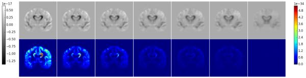
Mean and variance images for different values of α. Top: Mean images, Bottom: Variance images, Columns correspond to α values from left to right: 0.0, 0.01, 0.025, 0.05, 0.075, 0.1, and 0.5.

The sum of squared difference during registration

The initial sum of squared difference (SSD) between the screening and year 1 image was retained and used to normalize the SSD at every iteration. This normalized SSD was summed over all 57 image pairs. The results for all values of α are shown in Figure 2. Clearly, as α increases the total normalized SSD increases for every iteration, which is expected considering the forms of equations (7) and (10). As alpha increases, exact matching to the target is compromised for more coherence with the group-wise representation. The spikes occur where the resolution changes in the multi-scale registration approach.

Fig. 2.

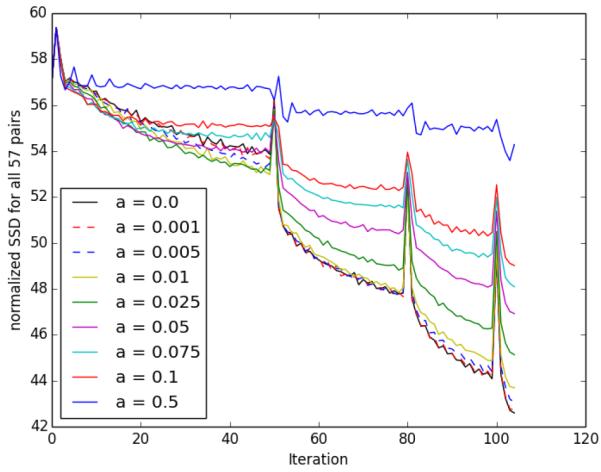
Normalized SSD throughout optimization for all values of α. The Spikes occur when the resolution changes.

Prediction of year 2 images from initial momenta

The momenta learned for all values of α were integrated from [0, 2], representing a 2 year period, and the screening images were transformed with the resulting diffeomorphisms. These images were quantitatively compared to actual year 2 follow up acquisitions. The SSD between the year 2 prediction and actual year 2 image, normalized by its value for α = 0.0, is presented in Figure 3. A value less than one indicates the prediction at a particular α level is closer by SSD than the prediction for α = 0.0. Clearly, for many images the prediction improves with increasing α. These images are those for which the true, unobserved, initial momenta lies closer to the group-wise mean. For some images, the prediction becomes worse with increasing α. These images are those for which the true, unobserved, initial momenta does not lie closer to the group-wise mean. An immediate extension of this work to address this issue is to modify (8) to allow for multiple subgroup-wise representations and/or to accommodate outliers.

Fig. 3.

SSD between year 2 images predicted by integration of initial momenta and actual year 2 image acquisitions for all 57 image pairs and all ln(α) values. The red stars represent the mean.

We performed a one-sided student’s t-test to determine if the SSD for predictions with α not equal to zero were significantly different from those with α equal to zero. All values of α except α = 0.5 have significantly different SSD values (at a standard significance level of p = 0.05) for their predictions. The relevant values are presented in Table 1.

Table 1.

t-test results comparing all α not equal to zero with α = 0 for SSD between year 2 prediction and acquired year 2 image. μ is the average difference between SSD values for α = 0 and α ≠ 0, σ is the standard deviation, T is the t-statistic, and p is the p-value. Recall, there were 57 image pairs. Significant results are bold.

α	0.001	0.005	0.01	0.025	0.05	0.075	0.1	0.5
μ	13.70	70.21	120.51	222.10	287.75	306.79	324.23	157.03
σ	52.25	143.67	278.01	586.49	953.82	1177.70	1335.04	2066.4
T	1.98	3.70	3.27	2.86	2.28	1.97	1.83	0.57
p	.026	.00025	.00092	.003	.013	0.027	0.036	0.29

Prediction of year 2 images from average momenta

The average momentum for all α in MDT coordinates was transformed into individual coordinates for the ith image pair using coadjoint transport through (ψⁱ)⁻¹. The resulting average momenta in individual coordinates were integrated over [0, 2], representing a 2 year period. The screening images were transformed with the resulting diffeomorphisms and the resulting images were compared to the actual year 2 acquisitions. The results are presented in Figure 4.

We performed a one-sided student’s t-test to determine if the SSD for predictions from the average momenta with α not equal to zero were significantly different from those with α equal to zero. All values of α have significantly different SSD values (at a standard significance level of p = 0.05) for their predictions. The relevant values are presented in Table 2.

Table 2.

t-test results comparing all α not equal to zero with α = 0 for SSD between year 2 prediction from average momenta and acquired year 2 image. μ is the average difference between SSD values for α = 0 and α! = 0, σ is the standard deviation, T is the t-statistic, p is the p-value. Recall, there were 57 image pairs. Significant results are bold.

α	0.001	0.005	0.01	0.025	0.05	0.075	0.1	0.5
μ	10.91	46.26	81.55	148.97	203.29	230.76	246.85	259.22
σ	9.04	37.91	67.28	127.07	179.47	207.67	224.56	249.41
T	9.11	9.21	9.15	8.85	8.55	8.39	8.30	7.85
p	2.22e-12	1.53e-12	1.92e-12	5.89e-12	1.82e-11	3.34e-11	4.69e-11	2.59e-10

4 Discussion

The first feature of the above presented methods and results to discuss is the obvious compromise between exact image pair matching and group-wise consistency represented by the parameter α. Figure 2 demonstrates the sensitivity of the exact image matching to this parameter. It’s interesting to note that the solution trajectory over iterations is very similar in shape for all values of α, though we get less exact matching as α increases as expected. Figure 3 and Table 1 demonstrate the potential advantage to group-wise consistency in learning momenta that more accurately reflect the unobserved long term change. Figure 3 and Table 1 both suggest that there are some values of α that strike a potentially desirable compromise between exact image matching and improved prediction of long term change.

Of course, for some images, the momenta learned with coupling are worse predictors of long term change. As mentioned previously, one avenue to address this is to allow multiple sub-group representations and assign each image pair to the sub-group representation that best approximates it. One interesting question that arises is what is the optimal number of sub-groups for a given population? Additionally, what differences will the sub-group representations encode in them after convergence? Alternatively, the mean is sensitive to outliers, and we could consider replacing the group representation with a different statistic more robust to such variation.

The proposed work has made no effort to normalize temporal misalignment in disease progression across patients. The experimental results suggest that AD disease progression is sufficiently similar at different stages of the disease for group level information to be applicable to individual trajectory estimation. However, this may not be the case for other populations such as the Mild Cognitively Impaired (MCI) or other Neurodegenerative disorders with less well characterized structural changes. Hence, explicit modeling of temporal misalignment in age and disease progression as done in [9] may improve results.

It is important to mention that momenta learned with this technique should not be naively used for statistical tests. We have explicitly minimized the trace covariance of these momenta, so any voxel-wise statistics computed from them are biased [11]. This issue can be compensated for by determining the null distribution for a particular statistic and establishing significance relative to this learned distribution. However, non-statistical inference applications such as momenta or change map atlas construction and shooting of individual templates via the learned momenta are not affected by this problem.

5 Conclusions

We have presented a mathematical framework for coupling the registration of N image pairs in the geodesic shooting approach for the optimization of the LDDMM energy functional. Individual registrations are coupled by maintaining a group-wise representation of their initial momenta and constraining updates to stay close to this representation. This is an explicit minimization of the variance of the initial momenta in the Lie algebra for the space of diffeomorphisms specified by the choice of metric K. This establishes a trade-off between exact image matching for individual image pairs and group-wise consistency. We’ve shown that increasing group-wise consistency can improve the prediction of long term change encoded within individual momenta. Finally, we have described some of the strengths and weaknesses of our initial choice for the coupling term G(.) and suggested methods to address those weaknesses.

References

- 1.Beg MF, Miller MI, Trouvé A, Younes L. Computing large deformation metric mappings via geodesic flows of diffeomorphisms. Int. J. Comput. Vision. 2005 Feb;61(2):139–157. http://dx.doi.org/10.1023/B:VISI.0000043755.93987.aa. [Google Scholar]
- 2.Brun CC, Lepore N, Pennec X, Chou YY, Lee AD, de Zubicaray GI, McMahon K, Wright MJ, Gee JC, Thompson PM. A nonconservative lagrangian framework for statistical fluid registration - safira. IEEE Trans. Med. Imaging. 2011;30(2):184–202. doi: 10.1109/TMI.2010.2067451. http://dblp.unitrier.de/db/journals/tmi/tmi30.htmlBrunLPCLZMWGT11. [DOI] [PubMed] [Google Scholar]
- 3.Iglesias J, Liu C, Thompson P, Tu Z. Robust brain extraction across datasets and comparison with publicly available methods. IEEE Transactions on Medical Imaging. 2011;30(9):1617–1634. doi: 10.1109/TMI.2011.2138152. [DOI] [PubMed] [Google Scholar]
- 4.James W, Stein C. Estimation with quadratic loss. Proceedings of the Fourth Berkeley Symposium on Mathematical Statistics and Probability, Volume 1: Contributions to the Theory of Statistics; Berkeley, Calif: University of California Press; 1961. pp. 361–379. http://projecteuclid.org/euclid.bsmsp/1200512173. [Google Scholar]
- 5.Lorenzi M, Pennec X, Frisoni GB, Ayache N. Disentangling Normal Aging from Alzheimer’s Disease in Structural MR Images. Neurobiology of Aging. 2014 Sep; doi: 10.1016/j.neurobiolaging.2014.07.046. [DOI] [PubMed] [Google Scholar]
- 6.Miller MI, Trouvé A, Younes L. Geodesic shooting for computational anatomy. Journal of Mathematical Imaging and Vision. 2006;24(2):209–228. doi: 10.1007/s10851-005-3624-0. [DOI] [PMC free article] [PubMed] [Google Scholar]
- 7.Niethammer M, Huang Y, Vialard FX. Geodesic regression for image timeseries. In: Fichtinger G, Martel AL, Peters TM, editors. MICCAI (2). Lecture Notes in Computer Science. Vol. 6892. Springer; 2011. pp. 655–662. http://dblp.uni-trier.de/db/conf/miccai/miccai2011-2.htmlNiethammerHV11. [DOI] [PMC free article] [PubMed] [Google Scholar]
- 8.Pennec X, Stefanescu R, Arsigny V, Fillard P, Ayache N. Riemannian elasticity: A statistical regularization framework for non-linear registration. MICCAI. 2005;8:943–950. doi: 10.1007/11566489_116. [DOI] [PubMed] [Google Scholar]
- 9.Singh N, Hinkle J, Joshi S, Fletcher P. A hierarchical geodesic model for diffeomorphic longitudinal shape analysis. Proceedings of the International Conference on Information Processing in Medical Imaging (IPMI). Lecture Notes in Computer Science (LNCS); 2013. [DOI] [PMC free article] [PubMed] [Google Scholar]
- 10.Trouve A. Diffeomorphisms groups and pattern matching in image analysis. 1998 [Google Scholar]
- 11.Tustison NJ, Avants BB, Cook PA, Kim J, Whyte J, Gee JC, Stone JR. Logical circularity in voxel-based analysis: Normalization strategy may induce statistical bias. Hum Brain Mapp. 2012 Nov; doi: 10.1002/hbm.22211. [DOI] [PMC free article] [PubMed] [Google Scholar]
- 12.Vialard FX, Risser L, Rueckert D, Cotter CJ. Diffeomorphic 3d image registration via geodesic shooting using an efficient adjoint calculation. Int. J. Comput. Vision. 2012 Apr;97(2):229–241. http://dx.doi.org/10.1007/s11263-011-0481-8. [Google Scholar]
- 13.Wei L, Awate S, Anderson J, Fletcher T. A functional network estimation method of resting-state fmri using a hierarchical markov random field. Neuroimage. 2014 Jun; doi: 10.1016/j.neuroimage.2014.06.001. [DOI] [PMC free article] [PubMed] [Google Scholar]
- 14.Yanovsky I, Thompson PM, Osher S, Leow AD. Topology preserving log-unbiased nonlinear image registration: Theory and implementation. In: CVPR. IEEE Computer Society. 2007 http://dblp.unitrier.de/db/conf/cvpr/cvpr2007.htmlYanovskyTOL07.
- 15.Younes L, Qiu A, Winslow RL, Miller MI. Transport of relational structures in groups of diffeomorphisms. Journal of Mathematical Imaging and Vision. 2008;32(1):41–56. doi: 10.1007/s10851-008-0074-5. http://dblp.unitrier.de/db/journals/jmiv/jmiv32.htmlYounesQWM08. [DOI] [PMC free article] [PubMed] [Google Scholar]
- 16.Zhang M, Singh N, Fletcher P. Bayesian estimation of regularization and atlas building in diffeomorphic image registration. 2013;23:586–591. doi: 10.1007/978-3-642-38868-2_4. IPMI. [DOI] [PMC free article] [PubMed] [Google Scholar]