Controlling False Discovery Rate in Signal Space for Transformation-Invariant Thresholding of Statistical Maps

Abstract

Thresholding statistical maps with appropriate correction of multiple testing remains a critical and challenging problem in brain mapping. Since the false discovery rate (FDR) criterion was introduced to the neuroimaging community a decade ago, various improvements have been proposed. However, a highly desirable feature, transformation invariance, has not been adequately addressed, especially for voxel-based FDR. Thresholding applied after spatial transformation is not necessarily equivalent to transformation applied after thresholding in the original space. We find this problem closely related to another important issue: spatial correlation of signals. A Gaussian random vector-valued image after normalization is a random map from a Euclidean space to a high-dimension unit-sphere. Instead of defining the FDR measure in the image’s Euclidean space, we define it in the signals’ hyper-spherical space whose measure not only reflects the intrinsic “volume” of signals’ randomness but also keeps invariant under images’ spatial transformation. Experiments with synthetic and real images demonstrate that our method achieves transformation invariance and significantly minimizes the bias introduced by the choice of template images.

1 Introduction

Mapping functional activation or genetic influence to brain anatomy involves hypothesis tests carried out at numerous voxel locations. Due to its stochastic nature, it is impossible to completely eliminate statistical errors, but at best to keep an appropriate balance between false positives and false negatives. If the threshold is too conservative, then true hints may be overlooked; if it is too liberal, then spurious claims may flood in, and accompanied with publication bias [16] towards positive results they will later mislead the research community to spend extra resources on hypotheses that do not exist in the first place.

A good threshold should be selected according to the amount of simultaneously conducted tests and an error rate criterion. Though an arbitrary uncorrected threshold may yield more “promising” results, its misgauged uncertainty may turn into pitfalls. A functional study in 2009 [5] illustrated that “significant” activation can be “detected” with uncorrected thresholds even in a dead salmon’s brain. Two widely used criteria are (1) the family wise error rate (FWER) [11] which is the probability that at least one error occurs in the results, and (2) the false discovery rate (FDR) [2,19] which, roughly speaking, is the expected portion of false discoveries among reported discoveries. Rather than prohibiting even a single error, the FDR provides a direct trade-off between detection power and error ratio, so since its debut in 1995 [2] it has been actively adopted.

Though multiple testing affects a broad range of modern science, from hunting genetic causes of complex diseases to correlating social factors with economic decisions, its application in statistical mapping is uniquely challenging because it involves both randomness and geometry. First, it essentially involves an infinite and uncountable number of tests residing on a continuous space, unlike a finite number of tests in genetic scans. Second, geometric operations and topological properties, such as spatial transformation and connected components, stand as important concerns. Moreover, spatial dependence among signals makes the problem highly complicated.

In this paper, we are particularly interested in transformation invariance in FDR control, especially for voxel-based FDR. We find it closely related to another important issue, spatial correlation, as discussed in Section 4. It is a popular practice to warp subjects’ images to a template space for statistical mapping, for example, the Talairach atlas [12], the LPBA40 atlas [18], the ICBM152 atlas [8] or customized atlases built with various software, such as ANTS, AIR, ART, Diffeomorphic Demons, FNIRT. As statistical mapping may take place in so many possible image spaces, it naturally raises a question: if we threshold a statistical map in two homogeneous spaces with the same FDR level, will their results be consistent under spatial transformation? If our methods are transformation variant, then our results may include the bias introduced by our arbitrary choice of atlases or registration software and parameters.

Since Genovese, Lazar, and Nichols [9] introduced the FDR to the neuroimaging community a decade ago, various adaptations and improvements have been made. However, transformation invariance, this highly desirable feature, has not been adequately addressed. To the best of our knowledge, this is the first paper dedicated to this topic. In Genovese et al.’s work (2002) [9], the FDR is the defined as the volumetric ratio of false positive regions again positive regions, and controlled by Benjamini and Hochberg’s step-up procedure [2,4] applied to voxel p-values. Nguyen et. al. (2014) [14] revisited Genovese et al.’s method [9], and reduced speckles with Markov random field. This voxel-based FDR definition has an obvious problem: if the image is spatially transformed, its volumetric measure will change and so does the FDR.

Pacifico et al. (2004) [15] pioneered to control the FDR for the number of clusters (which formally are connected excursion sets), instead of the volumetric ratio. He classified a cluster as false positive if its false positive volume exceeds a pre-defined ratio. Heller et. al. (2006) [10] then proposed a two-stage method: in the first stage, functional activated clusters are segmented with pilot data; then in the second stage, FDR control is applied to p-values derived from clusters’ average signals. Benjamini and Heller (2007) [1] later extended the method in [10] by weighting each cluster with its volumetric size. Though the number of clusters does not change under spatial transformation, these methods all partially rely on volumetric measure which is transformation variant: classification of false positive clusters by volumetric ratio in Pacifico et al.’s method [15], taking clusters’ average signals in Heller et. al.’s method [10], and weighting clusters with their sizes in Benjamini and Hochberg’s method [1].

Chumbley and Friston (2009) [7] and Chumbley et. al. (2010) [6] worked on random field theory. According to Gaussian random field theory, they calculated cluster p-values by either their sizes [7] or peak signals [6], and then they applied Benjamini and Hochberg’s step-up procedure [2,4] for FDR correction. Though these methods enjoy transformation invariance in their cluster-based FDR definition and p-value calculation, they introduced another problem: the number of clusters entering into the FDR stage, even pre-screened with a fixed threshold, becomes a random variable, while Benjamini and Hochberg’s methods [2,4] demand a fixed number of clusters. These methods then require the number of pre-screened clusters to be independent of cluster p-values, an assumption whose proof is unclear.

To achieve transformation invariance, we shall either define the FDR based on topological indices such as the number of clusters, or local properties such as local maximas, or if volumetric integration is involved, use a measure that does not change under transformation. Here we explore defining the measure in the signal space instead of the native image space. Although it is natural to define the measure directly in the image’s Euclidean space, spatial transformation and atlas choice affect this measure. Rather, the signal space is intrinsic and unaffected. We find that normalized residuals of a Gaussian multi-variate linear regression model uniformly distribute on a unit hyper-sphere independent of its regression statistics such as the t-statistics, F-statistics and p-values. Therefore, the image and the normalized residuals form a mapping from a Euclidean space to a unit hyper-sphere. We can define the volumetric measure as the “area” spanned by signals on the unit hyper-sphere. Because volumetric measure is involved in many aforementioned FDR methods [9,14,15,10,1], embedding our hyper-spherical measure could equip them with this highly desirable transformation-invariance feature.

In Section 2, we elaborate our method, including the unit hyper-sphere of normalized residuals, the weighted FDR, and the voxel-based FDR using signal space measure. In Section 3, we demonstrate with synthetic and real images that our method significantly reduces the bias introduced by spatial transformation. In Section 4, we discuss transformation invariance and signal’s spatial dependence.

2 Methods

2.1 Intrinsic Spherical Signal Space

We consider a linear model Y = Xβ + ε where X is an m-by-n (m > n) full column-rank matrix, Y is a column vector of length m, β is a column vector of length n, and ε_is (i = 1, ···, m) are identical and independently distributed (i.i.d.) variables following a Gaussian distribution N(0, σ²). In research applications, Y may be an fMRI time serials at a voxel location and X may be the design matrix of functional tasks, or in a tensor-based morphometry (TBM) study Y may be subjects’ Jacobian determinant at a voxel location and X may be a factor matrix of age, gender or disease states, etc. Please note:

• We assume that X is full column-rank so that the inverse of X^⊤X exists.

• We assume that m > n so that it is possible to estimate σ².

The maximum-likelihood and unbiased estimate of β is

$$\widehat{\beta }\equiv {(X^{\top }X)}^{-1}{X}^{\top }Y=\beta +{(X^{\top }X)}^{-1}{X}^{\top }\epsilon .$$

The residuals and the unbiased estimate of σ² are

$$\{\begin{array}{ll}\widehat{\epsilon }\hfill & \equiv Y-X\widehat{\beta }=\left[I-X{(X^{\top }X)}^{-1}{X}^{\top }\right]\epsilon ,\hfill \\ {\widehat{\sigma }}^2\hfill & \equiv \frac{{\widehat{\epsilon }}^{\top }\widehat{\epsilon }}{df},\text{where}df=m-n.\hfill \end{array}$$

Let us focus on the probabilistic and geometric properties of ε̂.

1. It follows a σ²-variance isotropic multi-variate Gaussian distribution embedded in the null space of X’s columns. More specifically, there exists an m-by-df matrix Z which satisfies X^⊤Z = 0 and Z^⊤Z = I, such that ε̃ ≡ Z^⊤ε̂~ N(0, σ²I_df×df) and ε̂= Zε̃.

2. It is independent of β̂.

3. Its normalized vector û = ε̂/|ε̂| uniformly distributes on a unit hyper-sphere in the null space of X’s columns, independent of σ² and σ̂².

Property 1 is the most insightful and it easily derives properties 2 and 3. We outline its proof as follows:

1. Because X is a full column-rank m-by-n matrix, its column null space has df = m − n dimensions.

2. Define Z as an m-by-df matrix whose columns are a set orthonormal bases of the null space of X’s columns. By definition, Z satisfies X^⊤Z = 0 and Z^⊤Z = I.

3. Define ε̃ ≡ Z^⊤ε̂, then this df-element random vector follows a Gaussian distribution N(0, σ²I_df×df), because:

   • ε̃ ≡ Z^⊤ε̂ = Z^⊤ [I − X (X^⊤X)⁻¹ X^⊤] ε = Z^⊤ε, as a linear combination of ε follows a multi-variate Gaussian distribution;

   • The expected value of ε̃ is Eε̃ = Z^⊤Eε = 0;

   • The variance of ε̃ is Eε̃ε̃^⊤ = E [Z^⊤εε^⊤Z] = Z^⊤E [εε^⊤]Z = Iσ².

4. Z also satisfies ZZ^⊤ = I − X (X^⊤X)⁻¹ X^⊤ because:

   • Both ZZ^⊤ [X Z] and [I − X (X^⊤X)⁻¹ X^⊤] [X Z] equal [0 Z];

   • [X Z] is a full-rank m-by-m matrix so its inverse exists;

   • Both ZZ^⊤ and [I − X (X^⊤X)⁻¹ X^⊤] equal [0 Z] [X Z]⁻¹.

5. ε̂ equals Zε̃ because

   $$\widehat{\epsilon }=\left[I-X{(X^{\top }X)}^{-1}{X}^{\top }\right]\epsilon =Z{Z}^{\top }\epsilon =Z\stackrel{\sim }{\epsilon }.$$

2.2 Weighted FDR in Volume

Let R_pos denote the detected region, R_tru the underlying truth, and |•| the volume of a region. The volume-based FDR is defined as follows

$$\mathit{FDR}\equiv E\left[\frac{\mid R_{\mathit{pos}}\backslash R_{\mathit{tru}}\mid }{\mid R_{\mathit{pos}}\mid }\right]\text{where}\frac{\mid R_{\mathit{pos}}\backslash R_{\mathit{tru}}\mid }{\mid R_{\mathit{pos}}\mid }\equiv 0\text{if}\mid R_{\mathit{pos}}\mid =0.$$ (1)

Genovese, Lazar, and Nichols [9] defined the volumetric measure in the image space, and consequently it can be translated as the number of voxels in voxel-based analysis. Benjamini and Hochberg’s step-up procedure [2] was applied to control the FDR. The step-up procedure finds

$$k^{\ast }=max\{k\mid \frac{p_{(k)}N}{k}\le q\},$$

where q is the user specified FDR level, p_(k) is the k-th smallest voxel p-value, and N is the number of voxels. This step-up procedure is able to handle positive dependence among tests, as Benjamini and Yekutieli discussed in [4]. For more general dependence among tests, please refer to [4].

Benjamini and Hochberg (1997) [3] upgraded it to a weighted version whose FDR and control procedure are

$$\mathit{FDR}\equiv E\left[\frac{{\sum }_{i\in R_{\mathit{pos}\backslash R_{\mathit{tru}}}}{w}_i}{{\sum }_{i\in R_{\mathit{pos}}}{w}_i}\right],k^{\ast }=max\{k\mid \frac{p_{(k)}{\sum }_{i=1}^N{w}_{(i)}}{{\sum }_{i=1}^k{w}_{(i)}}\le q\},$$ (2)

where w_i is the weight associated with a voxel.

2.3 FDR in Signal Space

If an image is spatially transformed, some voxels will expand and some will shrink, so does the volumetric measure of the positive and false positive regions. The weighted FDR provides us a way to exploit the signal space volumetric measure for transformation invariance. The normalized residual image u = f(x) (where x is a point and u is a normalized residual vector) defines a mapping from to (where D is the image’s dimension). Instead of defining |R_pos| and |R_tru| in , we define them in the unit space:

$${\mid R\mid }_{\mathit{sig}}={\int }_{x\in R}\sqrt{det[J^{\top }(x)J(x)]}dx,$$

where R stands for either R_pos or R_tru, and J(x) is the Jacobian matrix of the mapping at x. For voxel-based FDR implementation, we can assign each voxel i a weight $w_i=\sqrt{J^{\top }J}$ and then apply the weighted step-up procedure (2). For the calculation of J(x), instead of directly taking linear difference between a center u and its neighboring voxel value u^†, we first map u^† to u’s tangent plane:

$$v^{†}\equiv log(u^{†})\equiv \frac{u^{†}-ucos\phi }{\Vert u^{†}-ucos\phi \Vert }\phi ,\text{where}\phi =arccos(\langle u,u^{†}\rangle ).$$

The length of v^† is the length of the geodesic connecting u and u^† on and its direction is same as the initial velocity from u to u^†.

3 Experiments

The proposed method is tested with synthetic 2D brain images and real 3D brain images, in comparison with Genovese, Lazar, and Nichols’ [9] voxel-based FDR method using the image space measure. For convenience, we denote the two methods as sigFDR and volFDR respectively. We choose the method in [9] for comparison because it is the most straight-forward adaptation of FDR to statistical maps. In this way, we minimize influence introduced by other factors, such as Markov Random Field smoothing [14] or cluster pre-screening [10], but solely focus on the use of difference volumetric measures.

The experiments are performed in the following framework: vector-valued images are generated in its original space which we call the fixed image space, and then warped with linear interpolation to a new space which we call the moving image space. After FDR thresholding is applied at the 5% level in both the fixed and moving image spaces, the results in the two image spaces are compared. To evaluate the FDR, positive signals are added to some regions, so the ground truth is known in the image generation stage and the evaluation stage, but blind to the FDR thresholding stage. This procedure randomly repeats several times to estimate the expected value and standard deviation of performance indices. We span the signal to noise ratio (SNR) in a range to provide a broad view of the performance. The evaluation indices include:

• Image-wise consistency: Let P_fix and P_mov respectively denote the detected binary-valued image (where 1 stands for positive and 0 for negative) in the fixed and moving image spaces, and P_mov ∘ Φ the transformation of P_mov to the fixed image space with linear interpolation followed by thresholding at 0.5. Image-wise consistency, measured with the Dice index between P_fix and P_mov ∘ Φ, is

  $$\mathit{Dice}\equiv \frac{2{\sum }_{i\in \mathit{brain}}{P}_{\mathit{fix}}(i)\wedge P_{\mathit{mov}}\circ \mathit{\Phi }(i)}{{\sum }_{i\in \mathit{brain}}[P_{\mathit{fix}}(i)+P_{\mathit{mov}}\circ \mathit{\Phi }(i)]}.$$
• Image-wise detection power: Let T denote the binary image of the ground truth, and P a detection result in the same space. Image-wise detection power is

  $$\mathit{Power}=\frac{{\sum }_{i\in \mathit{brain}}P(i)\wedge T(i)}{{\sum }_{i\in \mathit{brain}}T(i)}.$$

  P_fix and P_mov ∘ Φ are respectively used as P and the truth image in the fixed image space is used as T.

• FDR: For P_fix and P_mov ∘ Φ, their FDR is calculated with Eq. (1).

• Voxel-wise consistency: The detection of a voxel in repetitive trials builds a binary vector. The detection consistency at a voxel location is the Dice index between the two binary vectors derived from P_fix and P_mov∘Φ.

• Voxel-wise detection power: The detection power at a voxel location is the ratio of its detection in the repetitive trials.

3.1 Experiment with Synthetic 2D Images

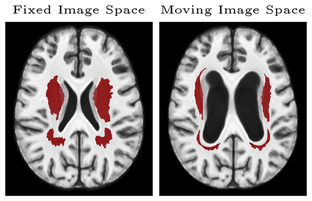
50 T1-weighted MR images are selected from the Philadelphia Neurodevelopmental Cohort (PNC) [17] to construct an 3D atlas. An axial slice of the atlas is extracted as the fixed image, and spatially transformed to generate the moving image. In each trial, 40 images filled with unit-variance white noises are simulated and then smoothed with a 4-voxel wide Gaussian kernel. Then, signals are added in the regions shown in Figure 1. The SNR ranges from 0.1 to 0.2. Voxel p-values are calculated with the two-sided t-test. 50 random trials are repeated.

Fig. 1.

Truth Images

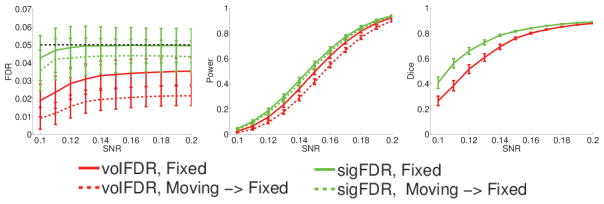
The image-wise FDR, detection power and consistency are shown in Figure 2. Both the sigFDR (green) and the volFDR (red) methods control the FDR, as measured in the fixed image space, around the target 5%. However, the volFDR shows considerable difference in its FDR and detection power between detection directly in the fixed image space (solid curves) and that warped back from the moving image space (dashed curves). On the other hand, the sigFDR shows much less difference. This is also evidenced by the Dice index plot.

Fig. 2.

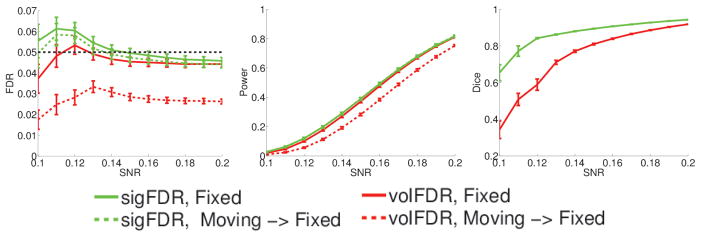
Image-wise performances evaluated in the fixed image space. Green and red curves respectively show the performance of the sigFDR and volFDR methods. In the FDR and Power plots, solid curves are for detection directly in the fixed image space, and dashed curves (except the black one) are for detection in the moving image space later warped back to the fixed image space. The dashed black curve is the target FDR value 5%. In the Dice plot, curves show the consistency between the detection taking place in the two image spaces.

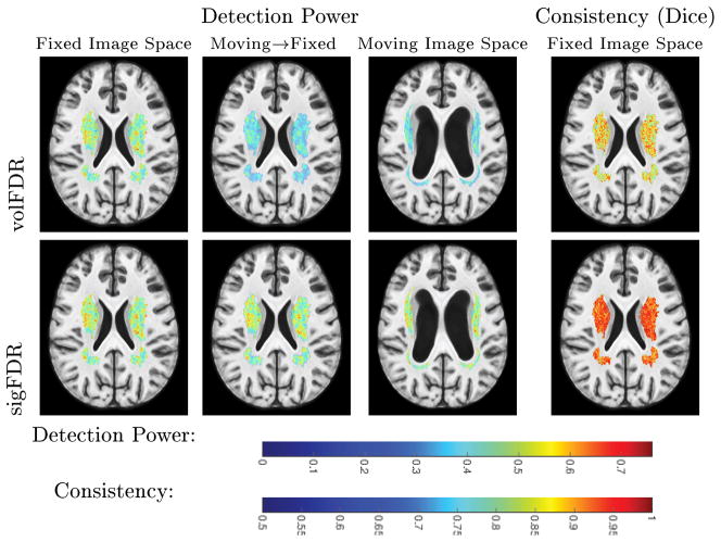
The voxel-wise detection power and consistency at SNR = 0.16 are shown in Figure 3. The power images of the volFDR method show considerable difference between the two image spaces, while the sigFDR results are much more consistent. The Dice images show clear evidence of the sigFDR method’s improved consistency.

Fig. 3.

Voxel-wise performances

3.2 Experiment with PNC Data

50 subjects are randomly selected from the Philadelphia Neurodevelopmental Cohort (PNC) [17]. The sampled subjects include 29 males (average age = 14.069 with std. = 3.741), and 21 females (average age = 15.4286 with std. = 3.9060). A 3D T1-weighted atlas is constructed and normalized Jacobian determinant maps are derived from TBM analysis for each subject. To build null hypotheses, we remove the linear effects contributed by both age and gender from the normalized Jacobian maps, but just utilize the residual images. Please note that the residual images still hold the non-homogeneous spatial dependence in the real data. 50 random trials are generated with bootstrap as follows. In each trial, 50 subjects are randomly re-sampled to replace the original residuals, and then signals (SNR=0.1~0.2) correlated with their ages are added to the hippocampus region, as shown in Figure 4. Voxel p-values are calculated with two-sided t-test to detect the effect of age. The hippocampus region is shrinked to produce moving images.

Fig. 4.

Truth Images

The image-wise FDR, detection power and consistency are shown in Figure 5. The sigFDR (green) controls the FDR more close to the target value 5% than the volFDR (red) does. The detection power of the volFDR decreases by about 7% in the moving image space (dashed curves), while that of the sigFDR only changes slightly. The sigFDR also gains 7%~20% absolute increase in the Dice consistency. The reader should note that it is possible for the volFDR to acheive higher detection power if the regions of interest expand instead of shrink. The key advantage of the sigFDR is its consistency under spatial transformation.

Fig. 5.

Image-wise performances evaluated in the fixed image space. Green and red curves respectively show the performance of the sigFDR and volFDR methods. In the FDR and Power plots, solid curves are for detection directly in the fixed image space, and dashed curves (except the black one) are for detection in the moving image space later warped back to the fixed image space. The dashed black curve is the target FDR value 5%. In the Dice plot, curves show the consistency between the detection taking place in the two image spaces.

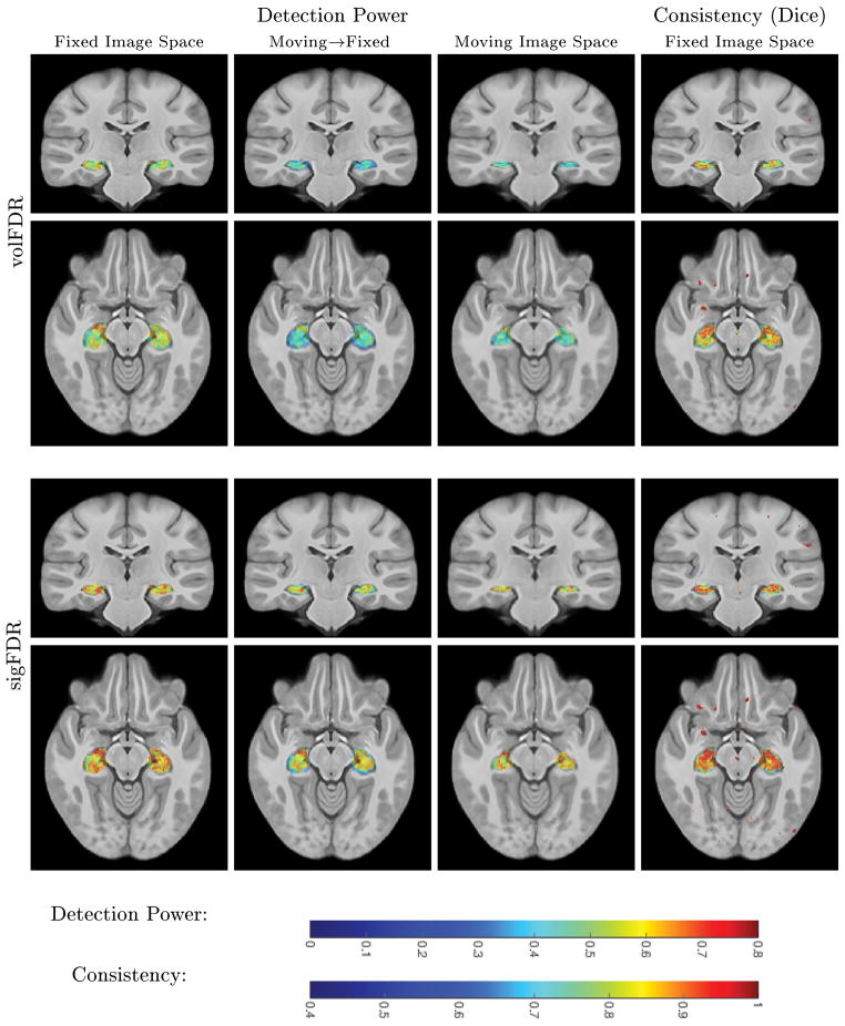
The voxel-wise detection power and consistency at SNR=0.15 are shown in Figure 6. The detection power of the volFDR decreases considerably in the moving image space, while the sigFDR method does not show significant changes. The sigFDR also achieves high voxel-wise consistency than the volFDR.

Fig. 6.

Voxel-wise performances

4 Discussions and Conclusions

We have shown in theory that defining volumetric measure in the intrinsic signal space can achieve transformation invariance in FDR control. Our experiments evidence the significant gain in consistency across thresholding taking place in different image spaces. (It should be noted that interpolation error may still affect consistency.) As volumetric measure is a fundamental component in FDR control, it can benefit many variations of spatial FDR control methods, for instance, those in [15,10,1,14], as we have already shown with Genovese, Lazar, and Nichols’ method [9]. Therefore, the relationship between our method and other methods are complementary rather than competitive.

Volumetric measure in the intrinsic signal space is also closely related to signals’ “effective volume of randomness”. Generally, the more tests are conducted simultaneously, the more stringent the p-values should be adjusted. Due to dependence among the tests, it may be over-conservative to adjust with the number of tests, but more suitable with the effective number of independent tests, as successfully demonstrated in many genetic studies [13]. In statistical mapping, the volumetric measure in signal space indicates the dispersion of signals on the unit hyper-sphere, and adjusts dynamically with signals’s spatial dependence.

Worsley (1999) [20] used resels to adjust the FWER of cluster sizes in random field theory. He assumed that the image space can be “flattened” to make signals’ spatial dependence homogeneous. It is unclear how to prove this assumption in general cases. Our method does not rely on such an assumption, but consider the normalized residual image as a mapping from a Euclidean space to a unit hyper-sphere. Worsley’s work was dedicated to signals’ spatial dependence and the FWER, while ours is for transformation invariance and the FDR, and also provides a thorough examination on the statistical and geometric properties of residuals. Putting these two works together, it is very clear that transformation invariance and spatial dependence are two closely related issues.

References

- 1.Benjamini Yoav, Heller Ruth. False discovery rates for spatial signals. Journal of the American Statistical Association. 2007 Dec;102(480):1272–1281. [Google Scholar]
- 2.Benjamini Yoav, Hochberg Yosef. Controlling the false discovery rate: A practical and powerful approach to multiple testing. Journal of the Royal Statistical Society. Series B (Methodological) 1995;57(1):289–300. [Google Scholar]
- 3.Benjamini Yoav, Hochberg Yosef. Multiple hypotheses testing with weights. Scandinavian Journal of Statistics. 1997 Sep;24(3):407418. [Google Scholar]
- 4.Benjamini Yoav, Yekutieli Daniel. The control of the false discovery rate in multiple testing under dependency. The Annals of Statistics. 2001;29(4):1165–1188. [Google Scholar]
- 5.Bennett CM, Miller MB, Wolford GL. Neural correlates of interspecies perspective taking in the post-mortem atlantic salmon: an argument for multiple comparisons correction. NeuroImage. 2009 Jul;47:S125. [Google Scholar]
- 6.Chumbley J, Worsley K, Flandin G, Friston K. Topological FDR for neuroimaging. Neuroimage. 2010 Feb;49(4):3057–3064. doi: 10.1016/j.neuroimage.2009.10.090. [DOI] [PMC free article] [PubMed] [Google Scholar]
- 7.Chumbley Justin R, Friston Karl J. False discovery rate revisited: FDR and topological inference using Gaussian random fields. Neuroimage. 2009 Jan;44(1):62–70. doi: 10.1016/j.neuroimage.2008.05.021. [DOI] [PubMed] [Google Scholar]
- 8.Fonov VS, Evans AC, McKinstry RC, Almli CR, Collins DL. Unbiased nonlinear average age-appropriate brain templates from birth to adulthood. NeuroImage. 2009 Jul;47:S102. [Google Scholar]
- 9.Genovese Christopher R, Lazar Nicole A, Nichols Thomas. Thresholding of statistical maps in functional neuroimaging using the false discovery rate. Neuroimage. 2002 Apr;15(4):870–878. doi: 10.1006/nimg.2001.1037. [DOI] [PubMed] [Google Scholar]
- 10.Heller Ruth, Stanley Damian, Yekutieli Daniel, Rubin Nava, Benjamini Yoav. Cluster-based analysis of FMRI data. NeuroImage. 2006 Nov;33(2):599–608. doi: 10.1016/j.neuroimage.2006.04.233. [DOI] [PubMed] [Google Scholar]
- 11.Hochberg Yosef, Tamhane Ajit C. Multiple comparison procedures. Wiley Series in Probability and Statistics. 1987 Sep; [Google Scholar]
- 12.Lancaster Jack L, Woldorff Marty G, Parsons Lawrence M, Liotti Mario, Freitas Catarina S, Rainey Lacy, Kochunov Peter V, Nickerson Dan, Mikiten Shawn A, Fox Peter T. Automated Talairach atlas labels for functional brain mapping. Hum Brain Mapp. 2000;10(3):120–131. doi: 10.1002/1097-0193(200007)10:3<120::AID-HBM30>3.0.CO;2-8. [DOI] [PMC free article] [PubMed] [Google Scholar]
- 13.Li J, Ji L. Adjusting multiple testing in multilocus analyses using the eigenvalues of a correlation matrix. Heredity. 2005 Aug;95(3):221–227. doi: 10.1038/sj.hdy.6800717. [DOI] [PubMed] [Google Scholar]
- 14.Nguyen Hien D, McLachlan Geoffrey J, Cherbuin Nicolas, Janke Andrew L. False discovery rate control in magnetic resonance imaging studies via Markov random fields. IEEE Trans Med Imaging. 2014 Aug;33(8):1735–1748. doi: 10.1109/TMI.2014.2322369. [DOI] [PubMed] [Google Scholar]
- 15.Perone Pacifico M, Genovese C, Verdinelli I, Wasserman L. False discovery control for random fields. Journal of the American Statistical Association. 2004 Dec;99(468):1002–1014. [Google Scholar]
- 16.Rosenthal Robert. The file drawer problem and tolerance for null results. Psychological Bulletin. 1979;86(3):638–641. [Google Scholar]
- 17.Satterthwaite Theodore D, Elliott Mark A, Ruparel Kosha, Loughead James, Prabhakaran Karthik, Calkins Monica E, Hopson Ryan, Jackson Chad, Keefe Jack, Riley Marisa, et al. Neuroimaging of the Philadelphia neurodevelopmental cohort. NeuroImage. 2014 Feb;86:544–553. doi: 10.1016/j.neuroimage.2013.07.064. [DOI] [PMC free article] [PubMed] [Google Scholar]
- 18.Shattuck David W, Mirza Mubeena, Adisetiyo Vitria, Hojatkashani Cornelius, Salamon Georges, Narr Katherine L, Poldrack Russell A, Bilder Robert M, Toga Arthur W. Construction of a 3D probabilistic atlas of human cortical structures. NeuroImage. 2008 Feb;39(3):1064–1080. doi: 10.1016/j.neuroimage.2007.09.031. [DOI] [PMC free article] [PubMed] [Google Scholar]
- 19.Storey John D. A direct approach to false discovery rates. Journal of the Royal Statistical Society. Series B (Statistical Methodology) 2002;64(3):479–498. [Google Scholar]
- 20.Worsley KJ, Andermann M, Koulis T, MacDonald D, Evans AC. Detecting changes in nonisotropic images. Hum Brain Mapp. 1999;8(2–3):98–101. doi: 10.1002/(SICI)1097-0193(1999)8:2/3<98::AID-HBM5>3.0.CO;2-F. [DOI] [PMC free article] [PubMed] [Google Scholar]