A Framework for Registration, Statistical Characterization and Classification of Cortically Constrained Functional Imaging Data

Abstract

We present a framework for registering and analyzing functional neuroimaging data constrained to the cortical surface of the brain. We assume as input a set of labeled data points that lie on a set of parameterized topologically spherical surfaces that represent the cortical surfaces of multiple subjects. To perform analysis across subjects, we first co-register the coordinates from each surface to a cortical atlas using labeled sulcal maps as constraints. The registration minimizes a thin plate spline energy function on the deforming surface using covariant derivatives to solve the associated PDEs in the intrinsic geometry of the individual surface. The resulting warps are used to bring the functional data for multiple subjects into a common surface atlas coordinate system. We then present a novel method for performing statistical analysis of points on this atlas surface. We use the Green's function of the heat equation on the surface to model probability distributions and thus demonstrate the use of PDEs for statistical analysis in Riemannian manifolds. We describe methods for estimating the mean and variance of a set of points, such that the mean also lies in the manifold. We demonstrate the utility of this framework in the development of a maximum likelihood classifier for parcellation of somatosensory cortex in the atlas based on current dipole fits to MEG data, simulated to represent a somatotopic mapping of S1 sensory areas in multiple subjects.

1 Introduction

Studies of brain activity often result in the detection of focal activated regions constrained to the cerebral cortex. For instance, current dipoles, representing focal neural current sources localized using MEG, can be constrained to lie on the cortical surface [1]. Meaningful analysis of these data requires methods that take into account the non-Euclidean geometry of the surface. For multiple subject analysis, assuming that parameterized representations of the surfaces are available, the problem can be reduced to two stages: (i) coregistration of the coordinate systems of each subject to a cortical atlas; and (ii) statistical analysis of the variability of these registered point sources in the intrinsic geometry of this atlas. For the purposes of this paper we select one representative cortical surface as the target or “atlas”. To register other individual cortical surfaces to this atlas, we solve the biharmonic equation using covariant derivatives to obtain a thin-plate spline warp from subject to atlas coordinates. The warp is constrained by a set of sulcal landmarks. Through use of covariant derivatives when solving the PDEs we make the resulting warp dependent only on the intrinsic geometry of the surface and independent of the specific parameterization. This approach is similar to that in [2] except that here we use a thin-plate spline rather than linear elastic energy resulting in a pair of decoupled PDEs, one for each component of the warping field. The resulting warp provides point to point correspondence between subject and atlas cortices by aligning their coordinate systems.

Once the surfaces have been registered, we can apply the same transformation to the functional point-source data so that we have a collection of points, all lying on the atlas surface, which we wish to analyze. The example we will use later in the paper is the location of the primary somatsensory area S1 for digits of the right hand as determined using magnetoncephalography. Mapping these areas for each subject to the atlas will give a collection of points for each digit reflecting the degree of variability of these functional areas in the surface space of the atlas. Our goal is to perform a statistical analysis of this variability.

Since the data are constrained to lie in a manifold, it makes sense to talk about an ‘average’ that is also constrained to lie in the manifold. Such an average can be called the ‘intrinsic mean’ [3,4]. More generally, we would like to define statistical distributions with respect to the manifold [5,6]. Since there is no simple notion of distance on the surface, averaging and quantifying variance in the intrinsic geometry is not straightforward. Note that geodesic distances are global rather than local attributes. We base our scheme on local attributes by using covariant PDEs, since in local neighborhoods, surfaces look like Euclidean spaces. Consequently it is possible to solve PDEs in the intrinsic geometry of the surfaces [7,8]. We use this idea to define statistical distributions on a manifold using the Green's function of the heat equation or the heat kernel. The heat kernel can be computed on any Riemannian manifold and reduces to a Gaussian function in Euclidean space. In this respect, our approach is a generalization of the use of Gaussian distributions from Euclidean to Riemannian spaces. Using this framework we describe methods for computing the mean and standard deviation of a set of points such that the mean itself lies on the surface. We then describe how to use these ideas to generate a maximum likelihood classifier in the intrinsic geometry of the cortical surface.

2 Surface Registration in the Intrinsic Geometry

2.1 Surface Extraction and Parameterization

We first extract cortical surfaces from MM for each subject using the Brainsuite software [9], which includes a 6 stage cortical modeling sequence. First the brain is extracted from the surrounding skull and scalp tissues using a combination of edge detection and mathematical morphology. Next the intensities of the MRI are corrected for shading artifacts. Each voxel in the corrected image is labeled according to tissue type using a statistical classifier. Coregistration to a standard atlas is then used to automatically identify the white matter volume, fill ventricular spaces and remove the brain stem and cerebellum, leaving a volume whose surface represents the outer white-matter surface of the cerebral cortex. It is likely that the tessellation of this volume will produce surfaces with topological handles. Prior to tessellation, these handles are identified and removed automatically using a graph based approach. The resulting mask is then tessellated to produce a genus zero surface.

We use our p-harmonic functional minimization scheme to map each cortical hemisphere onto a unit square. Our cortical flat maps are computed as described in [10]. Each brain hemisphere is mapped onto a unit square while constraining the interhemispheric fissure to lie on the boundary of the unit square. Let S denote the cortical surface. We assign a vector in R² to every point in the surface such that the two components denote the u and v coordinates assigned to that point, i.e. we define a vector-valued function ϕ : S → R². We chose the function ϕ to minimize the integral ∫_M‖∇ϕ‖^p where M denotes the integral over the hemisphere. The integral is discretized and minimized numerically using a conjugate gradient method to obtain a bijective p-harmonic map [10,11].

The square maps for each hemisphere are then resampled on a regular 256×256 grid, as illustrated in Fig 1. Because the interhemispheric fissure is fixed on the boundary of the square for each hemisphere, one can visualize the parameter space as two squares placed on each other and connected at the boundaries of the squares. This allows us to calculate partial derivatives across the two hemispheres and explicitly include the connectivity of the two cortical hemispheres in subsequent analysis. This boundary-less space is then used for solving the differential equations that will align the (u,v) coordinates of the sulcal features from the subject to the atlas space.

Fig. 1.

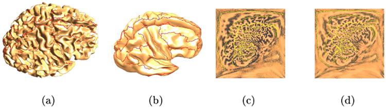
(a) A cortical surface with hand labeled sulci; (b) a smoothed version of the surface; (c) and (d) square p-harmonic maps of the left and right hemispheres. The interhemispheric fissure is constrained to lie on the boundary of the square.

The maps described above serve two purposes. First, they set up an initial alignment of the features across multiple subjects. Second, they are used as our computational space to align the cortices. However, thin plate spline based alignment uses covariant derivatives, and therefore is invariant with respect to the specific parameterization [12].

2.2 Thin Plate Splines in the Intrinsic Geometry of the Cortical Surface

Having parameterized each of the cortical surfaces, we now align coordinate systems between one surface, which we denote the “atlas”, and each of the other brain surfaces. The alignment uses a set of interactively labeled sulci, sampled uniformly along their lengths, as a set of point constraints [13]. To compute a smooth warping field ϕ from one coordinate system to the other we use the thin plate spline bending energy on the atlas surface as a regularizing function.

Thin plate (biharmonic) splines [14] have become a very popular method for landmark registration of 2D or 3D images. These splines are a generalization of the 1D cubic spline and correspond to the bending energy E_b of a thin metal plate:

$$E_b=\int {\left(\frac{{\partial }^2\varphi }{\partial x^2}\right)}^2+2{\left(\frac{{\partial }^2\varphi }{\partial x\partial y}\right)}^2+{\left(\frac{{\partial }^2\varphi }{\partial y^2}\right)}^2\mathit{\text{dxdy}}$$ (1)

We minimize this bending energy subject to the point landmark constraints, implemented here using a quadratic penalty function approach. Since we wish to minimize the bending energy in the surface, we must account for the intrinsic geometry of the surface when computing the integral. While we use the parameter space for doing the calculations required for evaluation of the bending energy, we account for the effect of the parameterization while calculating the integral. This is achieved using covariant derivatives which results in the property that given a set of homologous landmarks (initial alignment), the deformation is independent of the parameterization used for the computation of the TPS deformation field. The the use of covariant derivatives eliminates the effect of the initial parameterization on the resulting warping field.

We note that the eigenfunctions of the biharmonic operator on the surfaces are dependent on the surface itself. Therefore we cannot expand the deformations in terms of a common eigenfunction basis as in [14]. Instead we take a more direct approach and minimize the integral numerically. The bending energy is minimized in the intrinsic geometry after replacing the first and second partial derivatives in (1) by the corresponding covariant derivatives. This is explained in more detail in the Appendix. Integration over the surface can be carried out by integration in the parameter space while compensating with the surface metric g. The differential form ds² for the integration in the surface S is related to its counterpart in the parameter space (u, v) by ds² = gdudv. Let S be the set of all vertices, and let S_c denote the set of constrained vertices (landmarks). Let $d_j^1$ and $d_j^2$ denote the u and v displacements required at the j^th landmark, 1 ≤ j ≤ N, to take it to its location in the atlas space. The warping field (ϕ¹, ϕ²) with respect to the parameter space (u, v) that minimizes bending energy in the surface while matching the constraints is then given by:

$$\begin{array}{c}{\varphi }^1=arg\underset{{\psi }^1}{min}{\int }_P({({\psi }^1,11)}^2+{(\sqrt{2}{\psi }^1,12)}^2+{({\psi }^1,22)}^2)g\mathit{\text{dudv}},\text{with}{\varphi }^1(u_j,v_j)=d_j^1,\forall j\in S_c\\ {\varphi }^2=arg\underset{{\psi }^2}{min}{\int }_P({({\psi }^2,11)}^2+{(\sqrt{2}{\psi }^2,12)}^2+{({\psi }^2,22)}^2)g\mathit{\text{dudv}},\text{with}{\varphi }^2(u_j,v_j)=d_j^2,\forall j\in S_c\end{array}$$

We discretized the above integral in the parameter space over a 256×256 regular grid for each hemisphere. We denote the covariant differential operator in the above equations by L. As described previously, our parameter space takes into account the neighborhood relationships between the two hemispheres and thus the covariant operator L is discretized in such a way that derivatives at the interhemispheric fissure are calculated correctly. In our current implementation our constraints are enforced by adding a quadratic penalty term rather than the exact matching constraints in (2). Let Φ = (ϕ¹, ϕ²) denote the deformation field. The discretized cost function then takes the form

$$\Phi =arg\; min\sum _{i\in S}{\Vert \sqrt{g}{L}_i{\Phi }_i\Vert }^2+{\sigma }^2\sum _{j\in S_c}{\Vert \sqrt{g}(L_j{\Phi }_j-d_j)\Vert }^2$$

The resulting least squares problem is very high-dimensional (256×256×2×2 parameters), but it can be solved directly since the matrix L is sparse. However, we reduce the dimensionality of the problem by projecting onto a subset of the discrete cosine transform (DCT) basis functions. Provided the constraints can be satisfied with a relatively smooth deformation, this approach will work with fewer basis functions than the original 256×256 samples in (u, v) space. Let B denotes the DCT basis matrix, T = LB, Ψ = B^TΦ and T_i = L_iB. The optimization problem reduces to:

$$\begin{array}{c}\Phi =arg\; min\sum _{i\in S}{\Vert \sqrt{g}{L}_{i}B{B}^T{\Phi }_i\Vert }^2+{\sigma }^2\sum _{i\in S_c}{\Vert \sqrt{g}{L}_{i}B{B}^T{\Phi }_i-d_i\Vert }^2\\ \Psi =arg\; min\sum _{i\in S}{\Vert \sqrt{g}T\Psi \Vert }^2+{\sigma }^2\sum _{i\in S_c}{\Vert \sqrt{g}{T}_i\Psi -d_i\Vert }^2\end{array}$$

In this way, we calculate the deformations in DCT transform space. Use of this basis leads to a significant increase in speed. The warps thus obtained are then applied to the (u, v) coordinates of each cortical surface to coregister them to the template. This process is illustrated in Fig. 2 where we show the sulci traced on the original cortical surface and their corresponding locations in flat space. We then show the relative locations of these sulcal features in flat space for the subject and atlas before and after matching. Note that we use a quadratic penalty function to match the landmarks so that they do not exactly align after registration. Note also that cortical regions near the boundary of the unit square exhibit larger metric distortion relative to the cortical surface than do regions near the center. Since the warp bending energy is computed with respect to the intrinsic geometry of the surface rather than flat space, we see that the warp in flat space exhibits larger deformations near the boundaries than at the center, following the pattern of metric distortion.

Fig. 2.

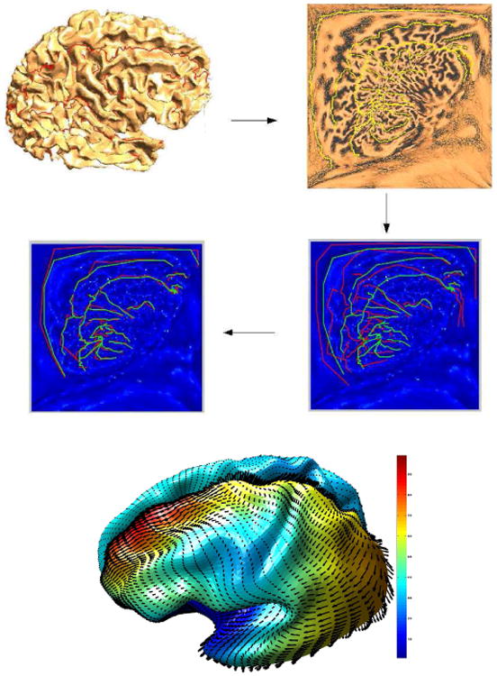
The intrinsic TPS warping process. The figure show the extracted cortex, its p-harmonic map, and sulci of the subject and atlas mapped to the parameter space before (right) and after (left) warping. The figure at the bottom shows the warping field computed on the surface. The color indicates the magnitude of the deformation.

3 Statistical Analysis in Riemannian spaces

We now turn to the problem of statistical analysis in the space of the cortical surface atlas. We describe a general approach to modeling statistical variability of points on this surface, and illustrate its application to pattern classification. In functional brain imaging, localized regions of activation can be constrained to lie on the cortical surface. Pattern classification of this data requires a classification scheme that considers the intrinsic geometry of the cortical surface. Here we present such a scheme based on a parametric model that extends the Gaussian distribution to Riemannian surfaces [15]. This approach uses the heat kernel to replace the Gaussian distribution so that a probability density function on the surface can be defined by analogy to heat propagation on a surface.

3.1 The heat equation in the intrinsic geometry

The heat equation in the intrinsic geometry of the surface is given by:

$$(\Delta -\frac{\partial }{\partial t})\zeta =0\text{where}\Delta =\frac{1}{\sqrt{g}}\frac{\partial }{\partial u^i}\sqrt{g}{g}^{ij}\frac{\partial }{\partial u^j}$$

where Δ denotes the Laplace-Beltrami operator and ζ is the scalar field being diffused. We discretized the operator using the metric tensor calculations described in the Appendix. Using this discretized operator, we set up the Crank-Nicolson scheme [16] for solving the heat equation since it is known to be stable. We illustrate the differences between using the usual Laplacian and the Laplace-Beltrami operator in Fig. 3. In the former, diffusion is computed with respect to the 2D Euclidean space and produces a 2D Gaussian distribution in the flat parameter space which maps to a clearly anisotropic distribution on the surface. Conversely, the Laplace-Beltrami form computes the diffusion directly on the surface, on which it produces an isotropic distribution while exhibiting anisotropic behavior with respect to the parameter space. Solutions of linear partial differential equations, such as the heat equation, can be characterized by Green's functions. The Green's function of the heat equation, also known as the heat kernel, has been a topic of extensive research in spectral theory [17]. Though the heat kernel can only be implicitly defined in arbitrary surfaces, several of its properties in Euclidean spaces extend to Riemannian spaces and, in particular, to surfaces.

Fig. 3.

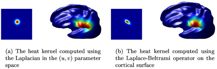
The heat kernels are displayed in the parameter space and on the surface. It can be seen that when the Laplace-Beltrami operator is used instead of the Laplacian, the heat kernel is not isotropic in the parameter space, however it is isotropic on the surface.

Here we list a few properties we will use later in this paper. Proofs can be found in [17]. Let M be a geodesically complete Riemannian manifold. Then the heat kernel K_t(x, y) exists and satisfies

1. K_t(x, y) = K_t(y, x)

2. lim_t→0K_t(x,y) = δ_x(y)

3. $(\Delta -\frac{\partial }{\partial t})K=0$

4. K_t(x, y) = ∫_M K_t−s(x, z)K_s(z, y)dz

5. $K_t(x,y)={\sum }_{i=0}^{\infty }{e}^{-{\lambda }_{i}t}{\varphi }_i(x){\varphi }_i(y)$

3.2 The heat kernel as a pdf

We know that the heat kernel is positive everywhere. It integrates to one on the manifold [18] and therefore it is a suitable candidate for modeling the probability density function of sample points lying in the manifold. Moreover, in Euclidean space, the heat kernel is identical to the Gaussian pdf. Therefore we propose replacing the Gaussian density with the covariant heat kernel in our surface-based analysis [15].

Just as we can characterize an isotropic Gaussian distribution in the Euclidean plane through its mean and standard deviation, so we can characterize distributions on the surface through mean and variance-like parameters that characterize the location of the heat kernel and the ‘time’ at which it is observed. Estimation of these parameters is in turn analogous to maximum likelihood parameter estimation, i.e. parameter estimation for a set of sample points on the surface can be viewed as the problem of finding the kernel of a covariant differential operator that best fits these points.

For isotropic distributions the corresponding heat kernel K(m, t) on a Riemannian manifold can be completely specified by two parameters: m, the location of the initial impulse, and the time t. Parameters m and t play the role of the mean and variance in the Gaussian case. Thus the probability of finding a sample at x is modeled as p(x|m, t) = K_t(m, x). So the problem of fitting the heat kernel in the given sample points can be reduced to the problem of estimating these two parameters of the heat kernel.

If the sample points are x_i, we define the likelihood function for m and t as:

$$L(m,t)=\prod _{n=1}^N{K}_t(m,x_i)$$

Because of property 2 above, K_t(m, x) can be calculated explicitly by placing a delta function at point m and solving the heat equation up to time t. The problem with this approach is that the parameter m (the location of the mean) is unknown. However, since the heat kernel is symmetric (property 1), we can instead place the delta function at the sample points x_i whose locations are known, rather than at the unknown mean location m, and running the heat equation up to time t. This allows us to explicitly compute the likelihood function (2) for a set of sample points x_i for any time point t. The values of m and t for which the likelihood function L(m, t) attains its maximum are then our estimates of the mean and variance.

To use this scheme for supervised classification of two clusters of points, we first compute ML estimates of the parameters (m₁, t₁) and (m₂, t₂) for the two clusters. We then define a likelihood ratio as the ratio of the two heat kernels: R = K₁(m₁, t₁)/K₂(m₂, t₂) and compute this ratio at each point on the surface. The surface is then partitioned into two regions R > 1 and R ≤ 1.

4 Applications and Results

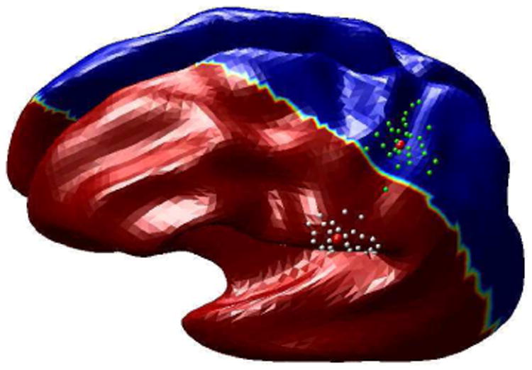
We illustrate the technique presented above for classification of point localizations of S1 somatosensory regions. For each of 5 subjects we simulated 6 points each representing locations of thumb and index figure on the postcentral gyrus; the 6 points could, for example, represent localizations from 6 separate studies on a single subject. We brought the cortical surfaces for all subjects into register, using one of the subjects as the atlas, as described above. We then used the pooled data from all subjects in the atlas-coordinates to compute the mean and standard deviation for the thumb and index finger respectively as illustrated in Fig. 4. We then applied the likelihood ratio statistic to partition the cortex as illustrated in Fig. 5. Note that this two-class problem classifies the entire brain, including both hemispheres, into two regions. With more somatosensory areas involved we could perform a finer partitioning of somatsensory cortex producing maps of the most probable areas to which each sensory unit would map. While this is a somewhat artificial problem, it is clear that an extension of this analysis would allow us to produce probabilistic maps of functional localization in the atlas space.

Fig. 4.

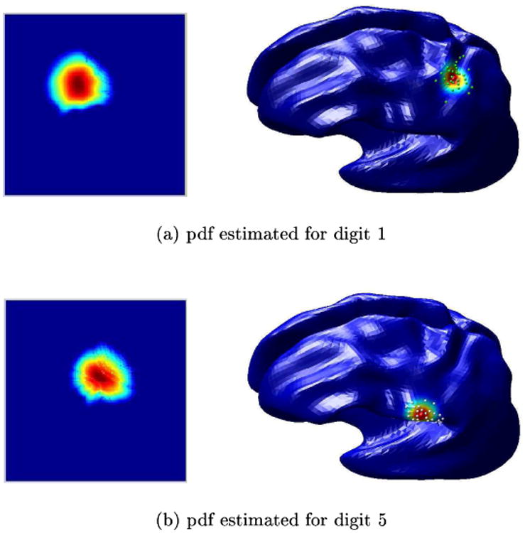
The figures shows the heat kernels estimated to fit the two datasets for MEG somatosensory data. For each of the datasets the estimated pdf is displayed in the parameter space and on the cortical surface.

Fig. 5. The classifier: Red and Blue regions shows the two decision regions.

5 Conclusion

We have presented a unified framework for analyzing cortically constrained functional data from multiple subjects where the analysis is performed in the intrinsic geometry of the surface. This allows us, for example, to compute the mean with respect to a cluster of points, such that the mean also lies in the surface. We have illustrated this framework by applying the analysis to produce functional parcellation of somatosensory cortex based on (simulated) MEG source localizations across multiple subjects. The method is currently limited to isotropic distributions and to point-wise analysis, but the idea of using the intrinsic heat equation, and kernels of covariant differential operators in place of the Gaussian distribution generalizes to the development of multivariate statistical analysis tools for data constrained to Riemannian manifolds.

Appendix

Let x denote the 3-D position vector of a point on the cortical surface. Let u¹, u² denote the coordinates in the parameter space. The metric tensor coefficients required in the computation are given by:

$$g_{11}={\Vert \frac{\partial \mathrm{x}}{\partial u^1}\Vert }^2,g_{22}={\Vert \frac{\partial \mathrm{x}}{\partial u^2}\Vert }^2,g_{12}=g_{21}=\langle \frac{\partial \mathrm{x}}{\partial u^1},\frac{\partial \mathrm{x}}{\partial u^2}\rangle ,g=g_{11}{g}_{22}-{(g_{12})}^2$$

Cartesian tensors suffice for flows in 2D or 3D Euclidean spaces. However the cortical surface is a two dimensional non-Euclidean space and from the outset demands a full tensorial treatment. We do this by replacing the usual partial derivatives by covariant derivatives. Although we want the deformation field with respect to the cortical surface to be independent of the specific choice of parameterization, the deformation field expressed in the 2D parameter space invariably does depend on the parameterization. Small deformations expressed in the parameter space can be modeled as contravariant vectors [19, 7] since, with respect to two different parameterizations u and ū, the respective values of the deformations ϕ and ϕ̄ are related by ${\overline{\varphi }}^{\beta }={\varphi }^j\frac{\partial {\overline{u}}^{\beta }}{\partial u^{\alpha }}$. In order to preserve their tensorial nature, we need to use covariant derivatives instead of the usual partial derivatives. The covariant derivative ${\varphi }_{,\sigma }^{\beta }$ of a contravariant tensor ϕ^β is given by:

$${\varphi }_{,\sigma }^{\beta }=\frac{\partial {\varphi }^{\beta }}{\partial u^{\sigma }}+{\varphi }^{\kappa }{{\Gamma }_{\kappa \sigma }}^{\beta }\text{where}\alpha ,\beta ,\kappa \in \{1,2\}$$

where Γ_κσ denote the Christoffel symbols of the second kind [7]. The first covariant derivative of a contravariant tensor ϕ^ζ is a mixed tensor ${\varphi }_{,\beta }^{\zeta }$. Covariant derivatives ${\varphi }_{,\beta \sigma }^{\zeta }$ of such a tensor is given by:

$${\varphi }_{,\beta \sigma }^{\zeta }=\frac{\partial {\varphi }_{,\beta }^{\zeta }}{\partial u^{\sigma }}-{\varphi }_{,\mu }^{\zeta }{{\Gamma }_{\beta \sigma }}^{\mu }+{\varphi }_{\beta }^{\nu }{{\Gamma }_{\nu \sigma }}^{\zeta }\text{where}\sigma ,\beta ,\mu ,\kappa \in \{1,2\}$$

References

- 1.George JS, Aine CJ, Mosher JC, Schmidt DM, Ranken DM, Schlitt HA, W CC, Lewine JD, Sanders JA, Belliveau JW. Mapping function in the human brain with magnetoencephalography, anatomical magnetic resonance imaging, and functional magnetic resonance imaging. J Clin Neurophysiol. 1995;12:406–431. doi: 10.1097/00004691-199509010-00002. [DOI] [PubMed] [Google Scholar]
- 2.Thompson PM, Hayashi KM, de Zubicaray G, Janke AL, Rose SE, Semple J, Doddrell DM, Cannon TD, Toga AW. Detecting dynamic and genetic effects on brain structure using high dimensional cortical pattern matching. Proceedings of ISBI. 2002 doi: 10.1109/ISBI.2002.1029297. [DOI] [PMC free article] [PubMed] [Google Scholar]
- 3.Fletcher PT, Lu C, Joshi SC. Statistics of shape via principal geodesic analysis on Lie groups. Conference on Computer Vision and Pattern Recognition. 2003;1:95–101. [Google Scholar]
- 4.Pennec X. Proc of Nonlinear Signal and Image Processing (NSIP'99) Antalya, Turkey: Jun 20-23, 1999. Probabilities and statistics on riemannian manifolds: Basic tools for geometric measurements. [Google Scholar]
- 5.Pennec X, Ayache N. Randomness and geometric features in computer vision; IEEE Conf. on Computer Vision and Pattern Recognition (CVPR'96); San Francisco, CA, USA. 1996; pp. 484–491. Published in J. of Math. Imag. and Vision 9(1), july 1998, p. 49-67. [Google Scholar]
- 6.Srivastava A, Klassen E. Bayesian and geometric subspace tracking. Adv in Appl Probab. 2004;36:43–56. [Google Scholar]
- 7.Kreyzig I. Differential Geometry. Dover: 1999. [Google Scholar]
- 8.Do Carmo M. Differential Geometry of Curves and Surfaces. Prentice-Hall; 1976. [Google Scholar]
- 9.Shattuck DW, Leahy RM. Brainsuite: An automated cortical surface identification tool. In: Delp SL, DiGioia AM, Jaramaz B, editors. MICCAI. Springer; 2000. pp. 50–61. Volume 1935 of Lecture Notes in Computer Science. [DOI] [PubMed] [Google Scholar]
- 10.Joshi AA, Leahy RM, Thompson PM, Shattuck DW. Cortical surface parameterization by p-harmonic energy minimization. ISBI. 2004:428–431. doi: 10.1109/ISBI.2004.1398566. [DOI] [PMC free article] [PubMed] [Google Scholar]
- 11.Eells J, Sampson JH. Harmonic mappings of Riemannian manifolds. Ann J Math. 1964:109–160. [Google Scholar]
- 12.Thompson PM, Mega MS, Vidal C, Rapoport J, Toga AW. Detecting disease-specific patterns of brain structure using cortical pattern matching and a population-based probabilistic brain atlas. Proc. 17th International Conference on Information Processing in Medical Imaging (IPMI2001); Davis, CA, USA. 2001; pp. 488–501. [DOI] [PMC free article] [PubMed] [Google Scholar]
- 13.Thompson PM, Toga AW. A surface based technique for warping 3-dimensional images of the brain. IEEE Transactions in Medical Imaging. 1996;15:1–16. doi: 10.1109/42.511745. [DOI] [PubMed] [Google Scholar]
- 14.Bookstein FL. Principal warps: Thin-plate splines and the decomposition of deformations. IEEE Transactions in Pattern Analyis and Machine Intelligence. 1989;11:567–585. [Google Scholar]
- 15.Hsu EP. Stochastic Analysis on Manifolds. American Mathematical Society; Providence, RI: 2002. [Google Scholar]
- 16.Smith GD. Oxford Applied Mathematics and Computing Science Series. 3. Oxford: Clarendon Press; 1985. Numerical solution of partial differential equations: Finite difference methods. [Google Scholar]
- 17.Rosenberg S. The Laplacian on a Riemannian manifold. Cambridge University Press; 1997. [Google Scholar]
- 18.Davies EB. Heat kernels and spectral theory. Cambridge University Press; 1989. [Google Scholar]
- 19.Thompson PM, Mega MS, Toga AW. Disease-specific probabilistic brain atlases. Procedings of IEEE International Conference on Computer Vision and Pattern Recognition; 2000; pp. 227–234. [DOI] [PMC free article] [PubMed] [Google Scholar]