

Abstract
This paper presents a complete overview of the electromagnetics (radiofrequency aspect) of MRI at low and high fields. Using analytical formulations, numerical modeling (computational electromagnetics), and ultrahigh field imaging experiments, the physics that impacts the electromagnetic quantities associated with MRI, namely (1) the transmit field, (2) receive field, and (3) total electromagnetic power absorption, is analyzed. The physical interpretation of the above-mentioned quantities is investigated by electromagnetic theory, to understand ‘What happens, in terms of electromagnetics, when operating at different static field strengths?’ Using experimental studies and numerical simulations, this paper also examines the physical and technological feasibilities by which all or any of these specified electromagnetic quantities can be manipulated through techniques such as B1 shimming (phased array excitation) and signal combination using a receive array in order to advance MRI at high field strengths. Pertinent to this subject and with highly coupled coils operating at 7 T, this paper also presents the first phantom work on B1 shimming without B1 measurements.
Keywords: B1 shimming, coil, electromagnetics, polarization, simulation, transmit array, ultrahigh field MRI
INTRODUCTION
To RF coil designers, the transition from low to high (≥3 T) and ultrahigh (≥7 T) field imaging has resulted in a similar transition from using circuit and transmission line theories (very specific cases of Maxwell’s equations) to using the more general and complete Maxwell’s electromagnetic theory. Following this notion, distributed circuit resonators have been used for human applications at and above 7 T, as exemplified by the transmission line resonator of Roschmann (1), the transverse electromagnetic (TEM) resonator of Vaughan (2), and the free element resonator of Wen (3). In contrast to lumped element designs, distributed circuit resonators utilize and enhance the transmission line properties of conductors by using the intrinsic reactance of transmission line elements. The electromagnetic interpretation of the behavior of loaded ultrahigh field distributed circuit coils as well as lumped-element based coil is still rather cumbersome due to the presence of the non-transverse electric/magnetic/electromagnetic (TEM/TE/TM) hybrid modes (4) and the differences between the transmit and receive fields (5,6).
This work presents a thorough view of understanding and manipulating the electromagnetics of MRI. The paper will first outline how and which electromagnetic components affect the MR signal. In the following sections, characteristics of the electromagnetic fields (global/local polarization and homogeneity) are examined at different field strengths and with different loading conditions. The paper then examines the modifications that need to be done on the typically obtained (during ultrahigh field imaging) electromagnetic transmit/receive fields to make them suitable (high and uniform) for the MR experiment. Simulations that aim at manipulating the B1 field (i.e. B1 shimming or phased array excitation) to achieve homogenous and/or localized RF excitation for imaging at 7 T are then presented. The paper then concludes with a brief section on new preliminary work in which a B1 shimming scheme fully based on rigorous computational modeling is successfully implemented on a whole-body 7 T system with a highly coupled coil and without any B1 measurements.
ELECTROMAGNETICS OF THE MRI SIGNAL
In this section we review the electromagnetic theory of the MRI signal, which was already discussed partially in Reference 7. Let us assume that a general electromagnetic field inside the human body/head is transmitted by a current on RF coil/transmit array. The magnetic field density of the B1 field can generally be defined (in terms of rms values in the frequency domain) as
| (1) |
Assuming the direction of the B0 field is in the +z direction, and using definitions and terms from the electromagnetic theory, the component that is responsible for exciting the spins during an NMR experiment is given as a circularly polarized component of the transverse magnetic field as follows:
| (2) |
With many assumptions described in details in References (7,8), at low flip angles the signal received in the MR experiment is linearly proportional to the product of the excite field (only the component that excites the spins) and the receive field given as
| (3) |
In Hoult’s rotating frames treatment of the MR signal derivation (8), a negatively rotating frame field was introduced such that1
| (4) |
The ‘receive field’ in his calculations was found to be equal to . In Ibrahim’s treatment which uses definitions and terms from electromagnetic theory (7), the ‘receive field’ given by the symbol was found to be the circularly polarized field with the opposite sense of rotation when compared to the field; specifically,
| (5) |
where the
field is a mathematical quantity that represents the circularly polarized component of the fictitious
 field, hypothetically induced by the receive coil. This component (
) would excite the magnetization of interest, if the
field were to be used for excitation (7).
field, hypothetically induced by the receive coil. This component (
) would excite the magnetization of interest, if the
field were to be used for excitation (7).
To relate the excite ( ) and the receive ( ) fields presented above to the typical definitions and terms of electromagnetic theory, the field can be defined as follows (7). For B0 = + |B0|z, the field is the circularly polarized component of the B1 field (produced by the transmit coil) in the counterclockwise (CCW) sense if the direction of the electromagnetic energy (direction of propagation) is +z; otherwise, it is the circularly polarized component of the B1 field in the clockwise (CW) sense if the direction of the electromagnetic energy is −z. If B0 = −|B0|z, the definition of the polarization sense of the field is reversed. For any specified receive coil, the sense of rotation of the field is always opposite to that associated with the field. The field would excite the spins if the receive coil was hypothetically used for that purpose.
The definitions of the excite and receive fields in MRI follow closely from reaction theory (9). The voltage induced in the antenna AA by another antenna BB is identical to that induced on BB by AA. Let us assume that AA is the receive coil (antenna) and BB is a magnetic current source resulting from the typically defined MRI transverse magnetization, i.e. the already excited spin(s) (7) (another antenna). Hypothetically, if we examine the voltage induced on BB due to AA, it is proportional to (1) a vector representing the polarization of the field that AA transmits and (2) the conjugate of a polarization vector that represents a field perfectly received by BB. The field that is perfectly received by BB is the field and the conjugate of it is the field. It is imperative to note that although the transmission is from AA (receive coil) to BB (magnetic current source/MRI transverse magnetization/excited spin(s)) in this situation (reaction theory), it is completely unrelated to the process of exciting the spins (7)2 as defined in MRI. An interesting observation about the antenna BB (excited spin(s)), however, is that it responds differently to electromagnetic components with the same sense of polarization if the associated waves are defined with different directions of propagation (using the electromagnetic theory definition). This is similar to a non-reciprocal antenna except, of course, in the near field region.
As both the components (the physical excitation field and the fictitious receive field) affect the MR image, in the following sections we will analyze and investigate how to manipulate both the and fields at different MRI static field strengths.
CHARACTERISTICS OF THE AND FIELDS AT DIFFERENT STATIC FIELD STRENGTHS AND LOADING CONDITIONS
The inhomogeneity of ultrahigh (≥7 T) field images at 7 (10,11), 8 (4,12), and 11.1 T (13) demonstrate that the RF excite ( ) and receive ( ) fields at such static field strengths are not well primed for human imaging. To achieve useful anatomical, physiological, and/or functional information, the and fields should possess high intensity (while not exceeding the RF power deposition limits) and uniformity in the specified region of interest. In order to achieve these characteristics, namely high intensity and uniform and fields, it is imperative to understand the electromagnetic principles of why these fields do not possess these characteristics at high static fields. Based on the nature of the and fields (circularly polarized electromagnetic field components), their desirable (from an MRI point of view) characteristics could be possibly hampered at high field strengths due to one or a combination of the following:
Issue 1: the electromagnetic fields induced (physically for transmit coil and/or fictitiously for receive coil) within the region of interest are not properly polarized.
Issue 2: the distribution of the and/or fields is/are inhomogeneous within the region of interest.
Issue 3: the intensity of field is low within the region of interest, thus leading to higher RF power deposition.
The following analysis (1,4,7,14) will address these three issues at different field strengths.
Effects of frequency and loading on RF field polarization (Issue 1)
A part of the discussion given in this section had already been presented in Reference (7). Let us assume a general transverse magnetic (B) field during MRI experiment. The total transverse field, CW and CCW (assuming +z propagation) components of the B field, are defined as follows:
| (6) |
| (7) |
| (8) |
Equations (7) and (8) demonstrate that with a negligible Bx (i.e. linear polarization) in the volume of the Tx/Rx coil, the CW and the CCW fields are equal in magnitude; hence, for MRI purposes, the distributions of and fields would be identical. This would not be the case if linear polarization is not present. Figure 1 displays the 3D finite difference time domain (FDTD) (15) solutions of different magnetic field intensities (6) inside a single element coil (6) operating under linear (1-port) excitation/reception. The results are presented for both an empty coil and a coil loaded with a small cylindrical phantom (9.4 cm long and 4.6 cm in diameter) at 254 MHz (6 T for 1H imaging) and 485 MHz (11.7 T for 1H imaging). The electromagnetic properties of the phantom were assigned to have a dielectric constant = 78 and conductivity = 1.154 S/m.
Figure 1.
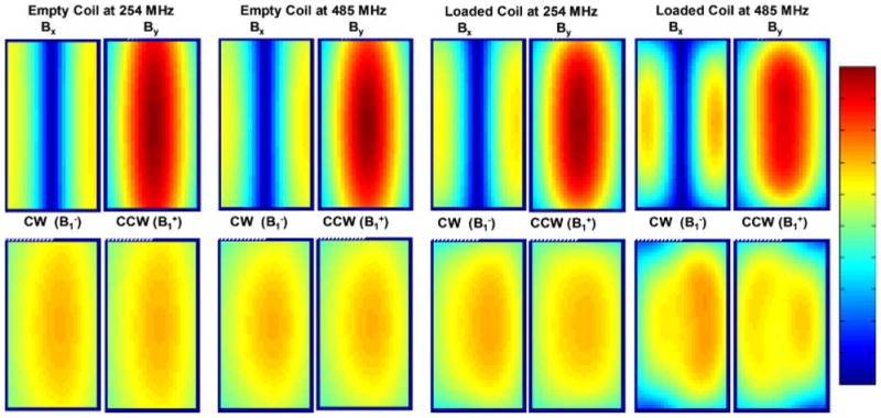
Calculated magnetic flux densities inside a single-strut TEM coil: empty and loaded with the cylindrical phantom at 254 MHz (6 T) and at 485 MHz (11.4 T). Bx and By represent the magnetic flux density in the x and y directions respectively, while CWW (proportional to ) and CW (proportional to ) correspond to the counterclockwise and clockwise circularly polarized components of the magnetic field, respectively. Reprinted with permission from Reference (6).
Figure 1 shows that the By field clearly dominates the transverse magnetic field (Bx is negligible) for the empty coil at both frequencies and for the loaded coil at 254 MHz. This evidently indicates that for these specific cases, linear excitation is clearly effective in producing linearly polarized fields3 (only By is present whereas Bx is negligible). Therefore, as shown in Fig. 1, the distributions of Bccw (i.e. ) and Bcw (i.e. ), fields are very much comparable.
When the dimensions of the coil and/or the load become a significant fraction of the operating wavelength, the electromagnetic interactions between the coil, drive port(s), and the load dominate the fields within the coil which may lead to the loss of linear polarization with linear excitation (16,17). This is demonstrated in Fig. 1 for the loaded coil at 485 MHz. In this case, Bx is not negligible when compared to By and therefore and field distributions of the coils are noticeably different.
In the following section, we will investigate the polarization and homogeneity of electromagnetic fields obtained for head sized ultrahigh field RF coils.
Effects of loading on global/local polarization and homogeneity for head imaging at ultrahigh fields (Issues 1–3)
A part of the discussion given in this section had already been presented in Reference (4). The previous section demonstrated that coil loading and increasing the operational frequency may contaminate the intended polarization. In this section, we will examine not only the extent of this contamination on polarization but also on the homogeneity of the and field distributions.
Figure 2 (4) displays FDTD calculated polarization vectors (vectors that contain characteristics of both polarization and intensity of the transverse magnetic field) which are presented (1) across a central axial slice at a single snapshot in time for a 16-element TEM coil (2) tuned to the typical operational mode and (2) in a local (close-up) area (approximately 16 mm2) at multiple time snapshots distributed throughout a complete cycle (i.e. 2π). The results are obtained for a linearly excited 16-strut TEM resonator tuned to 340 MHz under two loading conditions: loaded with an 18.5 cm diameter spherical phantom filled with 0.125 M NaCl solution (dielectric constant = 78 and conductivity = 1.154 S/m) (bottom) and empty (top). The data in the unloaded coil plots are shown in the central plane of the coil; this area has the same dimensions and is in the same location as the displayed slice for the loaded case. The intensities of the polarization vectors in this figure are represented by the lengths of the arrows while their directions (at instances in time) are represented by the tips of the arrows.
Figure 2.
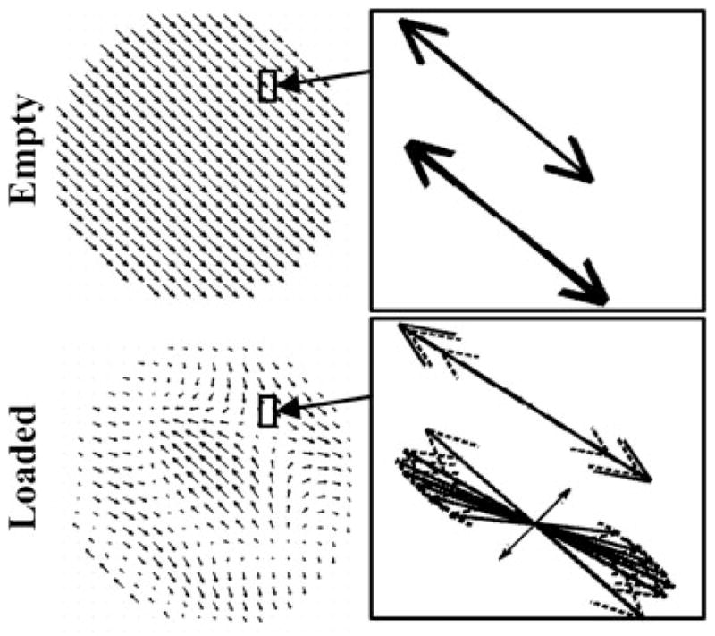
Axial slices of FDTD calculated vector field plots (polarization vectors) for (1) whole-slice (at a single snapshot in time) and (2) locally inside a 16 mm2 area (at many time snapshots forming a complete period, i.e. 2π) for mode 1 (the coil’s, 16-element TEM resonator, standard mode of operation). Reprinted with permission from Reference (4).
The whole-slice empty coil results shown in Fig. 2 clearly demonstrate that polarization vectors closely follow what is analytically obtained with transmission line and circuit theories (18,19). Specifically, at the center of the coil, mode 1 (typical mode of operation) possesses a non-zero polarization vector. As expected, the results of mode 1 also demonstrate that the direction and the intensity are nearly identical across the slice for all the polarization vectors. The local empty-coil polarization vectors results at multiple time snapshots also show that the two displayed polarization vectors are linearly polarized; i.e. they are always pointing in the ±45° direction with respect to the x or y axes. Hypothetically, if MRI could be performed with this particular empty TEM head coil tuned to 340 MHz (8T for 1H), highly uniform circularly polarized (transmit: and receive: ) fields will be obtained across the sample and will be achieved with 1/2 of the RF input power if quadrature excitation is used.
The behavior of the polarization vector in the loaded coil is quite different from that associated with the empty coil. The mode 1 whole-slice polarization data shown in Fig. 2 demonstrate that the intensities and directions of the polarization vectors are highly non-uniform across the slice (except in the central region of the slice), which will lead to non-uniform and fields. More importantly, however, the multiple time snapshots of mode 1 in the loaded coil reveal that within the 32 mm2 area shown in Fig. 2, the two displayed sets of vectors possess two different types of polarizations: linear (the tips of the vectors trace a line at all the time snapshots) and elliptical (the tips of the vectors trace an ellipse at all the time snapshots). Therefore in addition to the expected non-uniformity of the fields, linear excitation on ultrahigh field typical volume head coils results in linearly polarized fields in a few regions but not in the entire volume of the load. This in turn will result in a loss of circular polarization during two-port quadrature excitation as has been previously observed (6,16,20).
Based on above-mentioned observations, one can conclude that ultrahigh field imaging brings contamination of the MRI-intended polarization and of the homogeneity of the and field distributions. In addition, these two contaminations (1) are not necessarily bundled together in specific region(s) and (2) are also observed in selected regions across the volume of load and not over the whole volume.
The and fields: where and how much needs to be fixed
Some parts of the discussion given in this section were already presented in Reference (4). An attempt was then made to classify the volume of the above-mentioned spherical phantom and of a human head mesh (loaded in a TEM coil operating under linear excitation) (4,21) into 15 distinct regions: linear, elliptical (CW and CCW), and circular (CW and CCW) polarizations, as well as high, intermediate, and low intensities. At any voxel [(4 mm)3 for the spherical phantom, or (2 mm)3 for the human head mesh],
polarization classification criterion is defined as follows: linear: ξ ≤ 0.1, elliptical: 0.1 < ξ ≤ 0.9, and circular: ξ > 0.9, where ;
CW/CCW classification criterion is defined as follows: and , and
field intensity classification criterion is defined as follows: ; and , where and for linear and for circular and elliptical polarizations. Tables 1A and 1B provide the percentage of the volume of each region with respect to the total volume of the spherical phantom (1A) and the whole human head and neck mesh (1B). Figure 3 describes the distribution of these sections throughout each of the two loads.
Table 1.
Percentages with respect to the total volume of the coil load of 15 distinct regions that contain high, intermediate, or low intensity transverse magnetic field and linearly, elliptically (CW/CCW), or circularly (CW/CCW) polarized fields
| Elliptical
|
Circular
|
||||
|---|---|---|---|---|---|
| Percentage | Linear | CW | CCW | CW | CCW |
| A | |||||
| High | 22.3 | 11.9 | 11.9 | 0.0 | 0.0 |
| Intermediate | 16.0 | 18.5 | 18.5 | 0.3 | 0.3 |
| Low | 0.3 | 0.0 | 0.0 | 0.0 | 0.0 |
| B | |||||
| High | 1.5 | 4.8 | 5.7 | 0.0 | 0.0 |
| Medium | 18.1 | 29.3 | 30.7 | 0.5 | 0.1 |
| Low | 2.3 | 3.2 | 3.6 | 0.0 | 0.0 |
CW and CCW denote a clockwise and counterclockwise sense of rotation. The results are obtained numerically using the FDTD method inside a linearly excited 16 strut TEM resonator loaded with (A) an 18.5 cm diameter spherical phantom filled with 0.125 M NaCl or (B) the anatomically detailed human head mesh, and tuned to 340 MHz. Reprinted with permission from Reference (4).
Figure 3.
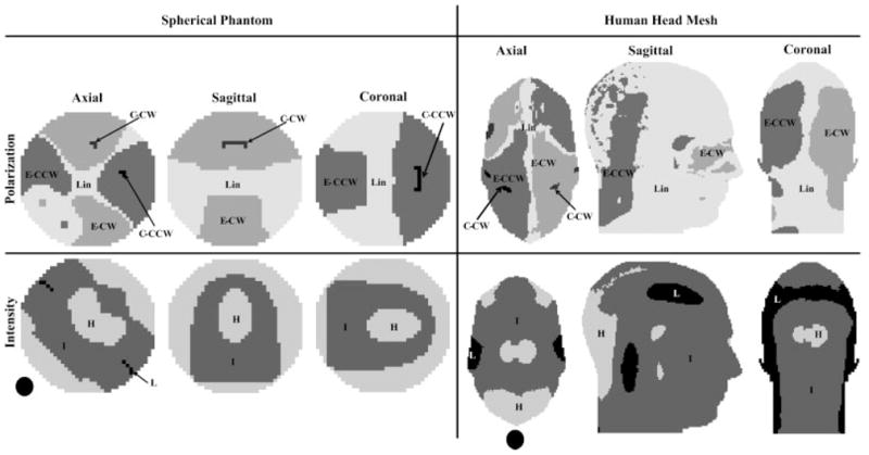
The 15 distinct regions provided in Table 1 for central axial, sagittal, and coronal slices. H, M, and L denote high, intermediate, and low intensities. Lin, C, and E denote linear, circular, and elliptical polarization. CW and CCW denote clockwise and counter clockwise sense of rotation (for the circular and elliptical polarization.) The black disc represents the location of the excited element. Reprinted with permission from Reference (4).
Case A: linear polarization and high and field intensities
Case A describes any region where the coil can both transmit and receive efficiently (high and comparable and field intensities); these include the central region of the coil/phantom/human head and neck mesh, the region near the drive port, and the region near the port opposite from the drive port. As shown in Fig. 3, the high intensity of both the and fields indicates a high intensity of the linearly polarized fields and consequently circularly polarized fields when quadrature excitation is used. Currently, during ultrahigh experiments with typical volume foils, regions falling under Case A have produced the most consistent and close to perfect excitation and reception. Tables 1A and Table 1B show that that these regions compose 22.3/1.5% of the total volume of the spherical phantom/human head and neck mesh. As expected and for verification purposes, this region was evaluated and was found to comprise 100% of a volume that is identical to that of the phantom inside an empty coil.
Case B: linear polarization and intermediate and field intensities
Figure 3 shows that Case B can be observed in the regions surrounding the central bright region of the spherical phantom/human head and neck mesh. In these regions, the fields possess intermediate intensity but maintain linear polarization. As a result, better NMR signal can be simply obtained by increasing the power in the transmit chain and by amplification in the receive chain. Table 1 shows that these regions comprise 16/18.1% of the total volume of the spherical phantom/human head and neck mesh.
Case C: linear polarization and low and field intensities
Case C describes load regions in which both transmission and reception are inefficient. Note that for mode 1 and linear excitation, the ratio of the maximum field intensity over the minimum field intensity for the whole spherical phantom volume was found to be approximately 100/1. However, when comparing the same ratio except considering and field intensities together at each voxel (i.e. every voxel in the phantom takes on the maximum of the two values), it was found to be 3.15/1. Hence, regions in which both transmission and reception are simultaneously inefficient are almost non-existent across the volume of the phantom. Table 1 and Fig. 3 show that these regions compose only 0.3/2.3% of the total spherical phantom/human head and neck mesh volume.
The insignificant volume associated with Case C is promising for imaging the head using ultrahigh fields with the ‘homogeneous’ mode of operation. If regions that possess weak (RF related) signal are observed during an ultrahigh field experiment with typical volume coils, they are a result of lack of intensity of the field or the field, but not of both fields. This signifies the existence of acceptable transverse magnetic (B1) field intensities across the majority of the load. This is not the case for ultrahigh field abdominal imaging, however (22).
Case D: elliptical polarization and high/intermediate and field intensities (two regions)
As shown in Fig. 3 and Table 1, Case D regions are spread out across the volume of the spherical phantom/human head and neck mesh, and form 60.8/70.5% of the spherical phantom/human head and neck mesh volume, as given in Table 1. Furthermore, regions with higher field intensities compared to field intensities or vice versa specify a particular sense of rotation, i.e. CW or CCW. Table 1A and B and Fig. 3 show that within Case D regions, two voxels within close proximity (few mms) can have elliptically polarized fields rotating in opposite senses (CW vs. CCW). In such regions (Case D), significant design changes, such as the use of B1 shimming (as will be demonstrated later) and/or transmit SENSE are needed to (1) obtain uniform field intensities and (2) re-polarize the electromagnetic fields closer to the eventually required circular polarization.
Case E: elliptical polarization and low and field intensities
Case E is almost non-existent throughout the phantom and only comprises 6.8% of the total human head and neck mesh volume.
Case F: circular polarization (three regions)
This case includes regions of low, intermediate, or high intensity circular polarization (where one of the field components ( or ) is much larger than the other). Regions that fall under Case F comprise only 0.6% of the spherical phantom/human head and mesh volume as shown in Fig. 3 and Table 1. While the percentage is quite small, it is nevertheless quite surprising that these regions exist at all for linear excitation at mode 1.
The above-mentioned analysis demonstrates that in terms of RF, the non-uniformity in ultrahigh field MR images is due to (1) RF field inhomogeneity and (2) loss of proper polarization. The following section will briefly show, using rigorous modeling techniques, how to experimentally and numerically manipulate the RF field in order to achieve a specific and/or field distribution(s) for ultrahigh field MRI.
MANIPULATING THE B1 FIELD (B1 SHIMMING) IN TRANSMIT/RECEIVE ARRAYS
The inhomogeneities of MR images and increased power deposition associated with high and ultrahigh field human imaging warranted new RF approaches (14,23–39) to overcome these issues. Early numerical work for potential high field MRI experiments has shown that specified superposition of electromagnetic fields radiated from long thin wires can alter the field in the sample (40) and that coil–head interactions could be manipulated by changing the coil’s excitation mechanism (21,29). This concept has been clearly verified in recent experimental head studies at 3, 7, and 9.4 T by varying the phases of the voltages driving the transmit array (23,41–43). As such, variable phase/amplitude multi-port excitation or B1 shimming (in electromagnetic terms, phased array antenna excitation) and other methods that manipulate the field such as transmit SENSE have been seen as possible solutions for achieving uniform and/or a specific field distributions (22,30,31,35,36,42,44–47) for high field MRI applications. These multi-transmit techniques have used many designs of transmit arrays (24,27,33,36,39,41, 44,48–57) (both coupled and uncoupled.)
Phased array excitation in MRI is based on the fact that for high frequency operation and asymmetrical/inhomogeneous/irregularly shaped loading (human head/body), integer multiples of phase-shifts and uniform amplitudes are not necessarily the ideal characteristics to impose on the voltages driving the transmit array to obtain a homogeneous transmit field. Furthermore, global as well as localized RF field excitations in high field human MRI may be achieved with rather distinctive and non-obvious amplitudes/phases. Using electromagnetic terms, the clear objectives of the phased array excitation in MRI are to (1) homogenize, (2) re-polarize, and (3) strengthen electromagnetic fields in specified regions of interest. These concepts will be evaluated in the following two sections.
NUMERICAL SIMULATIONS: THE POTENTIAL OF MANIPULATING THE B1 FIELD
Using in-house FDTD software (22,44), Fig. 4 demonstrates the potential of utilizing phased array excitation for ultrahigh field MRI (7 T). For example, Fig. 4 (top left) demonstrates not only a highly homogeneous RF excitation (as denoted by coefficient of variation) can be achieved with a 16-element highly coupled transmit array (TEM coil), but also it can be achieved simultaneously with lower (compared to quadrature, fixed phase/amplitude, excitation) total RF power absorption in the human head. Such findings indicate that re-polarization (correcting the polarization of the electromagnetic fields to strengthen of the field without increasing the total power deposition) can play a major role in B1 shimming.
Figure 4.
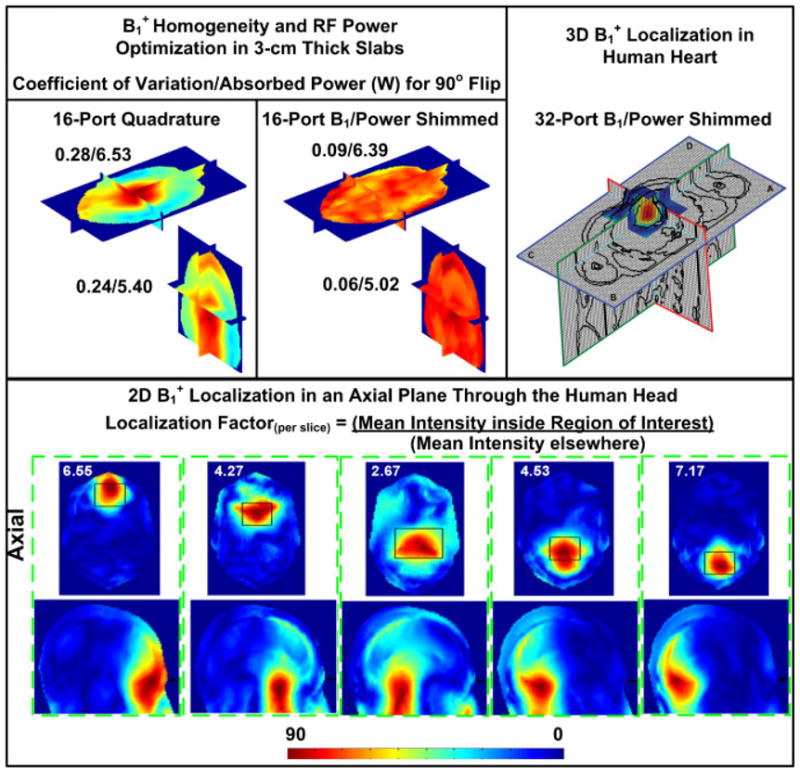
FDTD studies using highly coupled TEM resonators at 7 T. Top left: in-head field (flip angle) distribution using 16-port quadrature excitation (fixed phase, i.e. progressive phase shifts of 22.5° and constant amplitudes) and optimized phase/amplitude excitation (B1/power shimmed.) The optimization was targeted at minimizing the field distribution’s coefficient of variation in 3-cm axial and coronal slabs, while maintaining the total power absorption (in the human head model) lower than that obtained with 16-port quadrature excitation. Bottom: in-head localized excitation within whole-slices. Each black rectangle denotes a localized region of interest in which the mean field intensity everywhere else divided by the mean intensity within the same slice (‘localization factor’) is maximized. Spatial positions of the optimized regions were arbitrarily chosen. The value on each subfigure represents the ‘localization factor’. Each sagittal slice displayed below each axial slice (both are contained in a dotted green rectangle) contains the normalized flip angle distribution associated with the localized RF excitation in the corresponding axial slice. Position of the axial slice with respect to the sagittal slice is denoted by the black arrows. Reprinted with permission from Reference (44). Top right: axial, coronal, and sagittal slices through the heart and surrounding tissue in a specified rectangular volume showing the field distribution after 3D optimization was performed to localize the field in the heart. This was achieved by maximizing the average field intensity inside the heart over the average field intensity outside the heart and within a specified rectangular volume which is five times the heart’s volume. The average field intensity inside the heart over that outside the heart and contained within the specified rectangular volume was found to be 4.0 over 1.0. Reprinted with permission from Reference (22).
Figure 4 (bottom and top right) demonstrates that highly localized RF excitation field can be potentially achieved at 7 T for both head and abdominal imaging. In Reference (44) using the FDTD method, it was demonstrated that excellent homogenous whole-slice and localized (within slices) excitations can both be achieved in many regions of the human head at 7 T with the same transmit array. In Reference (22) and also using the FDTD method, 3D RF localized excitations in the human heart and 2D RF homogenous excitations in whole slices have been demonstrated for potential 7 T abdominal imaging. Such results were obtained by utilizing a 32-strut TEM resonator tuned to atypical mode, mode 2 (the third mode on the frequency spectrum.) These results and others (24,28,45,58) demonstrate that B1 shimming and transmit SENSE have a tremendous upside in ultrahigh field MRI.
To date, however, manipulating the field has been performed with highly decoupled transmit arrays by experimentally extracting the field and then utilizing optimization methods that aim at homogenizing and/or localizing the measured field. In the next section, we will briefly demonstrate our successful first attempt at performing B1 shimming (not only on the field but also on the receive, , field) without any B1 measurements using a highly coupled TEM coil loaded with a spherical head-sized phantom at 7 T.
EXPERIMENTAL MANIPULATION OF THE ELECTROMAGNETIC FIELDS: A PRELIMINARY LOOK AT B1 SHIMMING WITHOUT B1 MEASUREMENTS
Utilizing a rigorous (4,22) FDTD model that implements a true coaxial excitation (59), we have developed an eight-element, half-capped, TEM resonator model (highly coupled coil). The simulations at 7 T were performed using a 17.5 cm diameter spherical phantom as the load. The dielectric properties of the phantom were assigned to be approximately 80 for the dielectric constant and 0.46 S/m for the conductivity. The simulations utilized a four-port transmit/receive configuration where every other coil element was excited and was utilized in reception as well. As true coaxial excitation was utilized, the precise coupling between the coil elements is considered and the concept of super position can be implemented on the four transmit/receive ports. The simulated coil design and the phantom were constructed and built to the specifications of the simulations. To ensure the accuracy of the coil model, low and high flip angle 7 T experimental (acquired by using the University of Pittsburgh’s 7 T whole-body system) and FDTD simulated, at 298 MHz, images of axial, sagittal, and coronal slices of the phantom, loaded within the linearly (one port transmit/receive) excited TEM resonator, were obtained and compared as shown in Fig. 5. The results demonstrate the excellent accuracy of the FDTD model.
Figure 5.
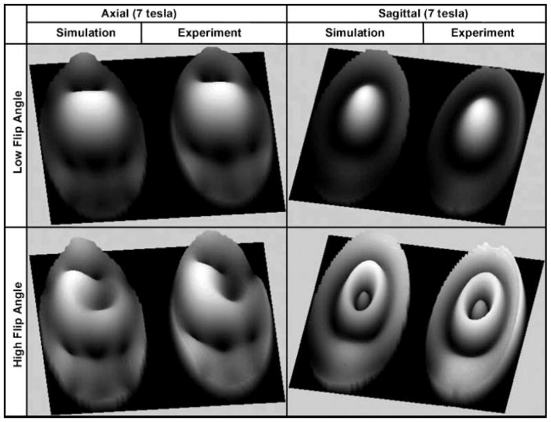
Axial, sagittal, and coronal low and high flip angle images obtained at 7 T and their corresponding simulated results obtained at 298 MHz using the rigorous FDTD model. The coil used was an 8-element TEM resonator excited in one port and tuned to its typical mode of operation and the load utilized in the experiments and numerical modeling was a 17.5 cm diameter spherical phantom with dielectric properties that are approximately 80 for the dielectric constant and 0.46 S/m for the conductivity.
Using the rigorous FDTD model, a four-port quadrature excitation/reception was simulated. Additionally, B1 shimming using constant amplitudes and variable phase shifts (optimized for both the and fields) was numerically executed to localize the low flip angle signal, i.e. maximize the mean of in regions of interest over the mean of elsewhere in the axial and sagittal planes. To implement constant amplitude and variable phase excitation/reception on the 7 T system, the 7 T transmit voltage was split into four different ways utilizing three quad-hybrids and high power three 50Ω loads. The quadrature and optimized RF localization (recommended from the simulations and without B1 measurements) phase conditions were achieved by constructing custom-made semi-rigid cables of specified length.
Figure 6 displays low flip angle images obtained by using the 7 T system and simulated using the rigorous FDTD model for four-port quadrature and optimized excitation/reception conditions. The circular loops in Fig. 6 represent the chosen (by the FDTD simulations) regions of interest. The preliminary results shown in Fig. 6 demonstrate that by properly modeling the load, transmit/receive array, and the excitation/reception scheme, B1 shimming (both and ) can be (1) guided through computational electromagnetics with minimal computational time requirements (seconds) and (2) efficiently implemented without any B1 measurement. These developments can pave the way for a fully automatic, subject specific, B1 homogenization/localization scheme for ultrahigh field human MRI (solutions to removing the effect of subject-specificity on B1 shimming without B1 measurements are presented in reference 43).
Figure 6.
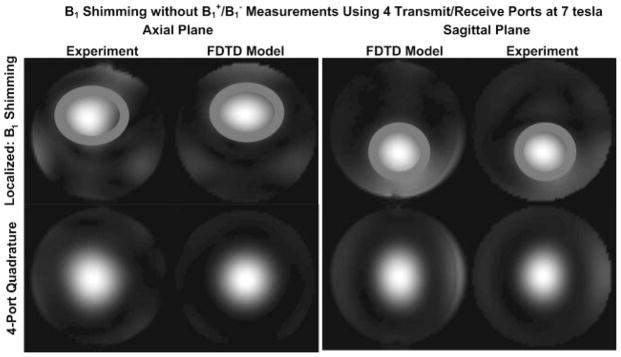
Axial and sagittal low flip angle images obtained at 7 T and their corresponding simulated results obtained at 298 MHz using the rigorous FDTD model. The transmit/receive array used was an 8-strut, highly coupled (approximately −10 dB coupling between the coil ports), TEM resonator that transmits and receives from four ports. The images were obtained using four-port quadrature and B1 shimming (on the transmit and receive chains) and with a 17.5 cm, in diameter, spherical phantom with dielectric constant = 80 and conductivity = 0.46 S/m as the load. The B1 shimming aimed at localizing the MR signal ( ) in the denoted gray circles. The phases of the B1 shimming were fully and completely obtained from the rigorous FDTD model without any B1 measurements and were implemented using specified semi-rigid coaxial cables to achieve the intended phases.
CONCLUDING REMARKS
The behavior of the electromagnetic fields during high/ultrahigh field MRI experiment may seem intricate and difficult to understand, however the electromagnetic waves in question are always governed by four basic and arguably simple equations: Maxwell’s equations. The proper application of these equations, i.e. electromagnetic theory, whether obtained through numerical and/or analytical approaches will always dictate the design, performance, and the safety of the RF excitation/reception during the MRI experiment. If we find differences between experimental observations and what is predicted by electromagnetic theory, it is more likely due to our misapplication of the theory, which unquestionably is sufficiently practical to fully and accurately handle the RF aspect of MRI. It is hoped that this paper can be used as a resource for understanding and manipulating the electromagnetic fields during MRI experiment.
Abbreviations used
- CCW
counterclockwise
- CW
clockwise
- FDTD
finite difference time domain
- RF
radio frequency
- TE
transverse electric
- TEM
transverse electromagnetic
- TM
transverse magnetic
Footnotes
The negative sign was changed to positive to follow the notation of this paper.
Maxwellian analysis shows that excitation of the spins is not reciprocal.
This generally indicates that quadrature excitation will be effective in producing the MR-desirable circularly polarized field.
References
- 1.Roschmann PK. US Patent 4,746,866. High-frequency coil system for magnetic resonance imaging apparatus patent. 1988
- 2.Vaughan JT, Hetherington HP, Otu JO, Pan JW, Pohost GM. High-frequency volume coils for clinical NMR imaging and spectroscopy. Magn Reson Med. 1994;32(2):206–218. doi: 10.1002/mrm.1910320209. [DOI] [PubMed] [Google Scholar]
- 3.Wen H, Chesnick AS, Balaban RS. The design and test of a new volume coil for high field imaging. Magn Reson Med. 1994;32:492–498. doi: 10.1002/mrm.1910320411. [DOI] [PMC free article] [PubMed] [Google Scholar]
- 4.Ibrahim TS, Mitchell C, Abraham R, Schmalbrock P. In-depth study of the electromagnetics of ultrahigh-field MRI. NMR Biomed. 2007;20(1):58–68. doi: 10.1002/nbm.1094. [DOI] [PubMed] [Google Scholar]
- 5.Wang J, Yang QX, Zhang X, Collins CM, Smith MB, Zhu XH, Adriany G, Ugurbil K, Chen W. Polarization of the RF field in a human head at high field: a study with a quadrature surface coil at 7.0 T. Magn Reson Med. 2002;48(2):362–369. doi: 10.1002/mrm.10197. [DOI] [PubMed] [Google Scholar]
- 6.Ibrahim TS, Mitchell C, Schmalbrock P, Lee R, Chakeres DW. Electromagnetic perspective on the operation of RF coils at 1.5–11.7 Tesla. Magn Reson Med. 2005;54(3):683–690. doi: 10.1002/mrm.20596. [DOI] [PubMed] [Google Scholar]
- 7.Ibrahim TS. Analytical approach to the MR signal. Magn Reson Med. 2005;54(3):677–682. doi: 10.1002/mrm.20600. [DOI] [PubMed] [Google Scholar]
- 8.Hoult DI. The principle of reciprocity in signal strength calculations—a mathematical guide. Concepts Magn Reson. 2000;12(4):173–187. [Google Scholar]
- 9.Balanis C. Advanced Engineering Electromagnetics. John Wiley; New York: 1989. [Google Scholar]
- 10.Vaughan JT, Garwood M, Collins CM, Liu W, DelaBarre L, Adriany G, Andersen P, Merkle H, Goebel R, Smith MB, Ugurbil K. 7 T vs. 4 T: RF power, homogeneity, and signal-to-noise comparison in head images. Magn Reson Med. 2001;46(1):24–30. doi: 10.1002/mrm.1156. [DOI] [PubMed] [Google Scholar]
- 11.Wald LL, Wiggins GC, Potthast A, Wiggins CJ, Triantafyllou C. Design considerations and coil comparisons for 7 T brain imaging. Appl Magn Reson. 2005;29(1):19–37. doi: 10.1002/mrm.20547. [DOI] [PubMed] [Google Scholar]
- 12.Kangarlu A, Baertlein BA, Lee R, Ibrahim T, Yang L, Abduljalil AM, Robitaille PM. Dielectric resonance phenomena in ultra high field MRI. J Comput Assist Tomogr. 1999;23(6):821–831. doi: 10.1097/00004728-199911000-00003. [DOI] [PubMed] [Google Scholar]
- 13.Beck BL, Jenkins K, Caserta J, Padgett K, Fitzsimmons J, Blackband SJ. Observation of significant signal voids in images of large biological samples at 11.1 T. Magn Reson Med. 2004;51(6):1103–1107. doi: 10.1002/mrm.20120. [DOI] [PubMed] [Google Scholar]
- 14.Nam H, Wright S, Grissom W, Noll D. Application of RF current sources in transmit SENSE. Seattle: May, 2006. p. 2562. [Google Scholar]
- 15.Yee KS. Numerical solutions of the initial boundary value problems involving Maxwell’s equations in isotropic media. IEEE Trans Ant Prop. 1966;14:302–317. [Google Scholar]
- 16.Ibrahim TS, Lee R, Baertlein BA, Kangarlu A, Robitaille PML. On the physical feasibility of achieving linear polarization at high-field: a study of the birdcage coil. ISMRM Meeting; Philadelphia, PA. 1999. p. 2058. [Google Scholar]
- 17.Ibrahim TS, Lee R, Baertlein BA, Yu Y, Robitaille PM. Computational analysis of the high pass birdcage resonator: finite difference time domain simulations for high-field MRI. Magn Reson Imaging. 2000;18(7):835–8843. doi: 10.1016/s0730-725x(00)00161-2. [DOI] [PubMed] [Google Scholar]
- 18.Tropp J. The theory of the bird-cage resonator. J Magn Reson. 1989;82(1):51–5162. [Google Scholar]
- 19.Glover GH, Hayes CE, Pelc NJ, Edelstein WA, Mueller OM, Hart HR, Hardy CJ, O’Donnell M, Barber WD. Comparison of linear and circular polarization for magnetic resonance imaging. J Magn Reson (1969) 1985;64(2):255–270. [Google Scholar]
- 20.Ibrahim TS, Lee R, Baertlein BA, Kangarlu A, Robitaille PML. Comparison between linear, quadrature, and 4-port excitations from 1.5 T to 4.7 T. ISMRM Meeting; Philadelphia, PA. 1999. p. 423. [Google Scholar]
- 21.Ibrahim TS, Lee R, Baertlein BA, Abduljalil AM, Zhu H, Robitaille PM. Effect of RF coil excitation on field inhomogeneity at ultra high fields: a field optimized TEM resonator. Magn Reson Imaging. 2001;19(10):1339–1347. doi: 10.1016/s0730-725x(01)00404-0. [DOI] [PubMed] [Google Scholar]
- 22.Abraham R, Ibrahim TS. Proposed radiofrequency phased-array excitation scheme for homogenous and localized 7-Tesla whole-body imaging based on full-wave numerical simulations. Magn Reson Med. 2007;57(2):235–242. doi: 10.1002/mrm.21139. [DOI] [PubMed] [Google Scholar]
- 23.Vernickel P, Findeklee C, Röschmann P, Leussler C, Overweg J, Graesslin I, Luedeke K, Katscher U, Schuenemann K. An eight channel transmit/receive body coil for 3 T. IMSRM Meeting; Seattle. May 2006; p. 123. [Google Scholar]
- 24.Wald L, Roell S, Fontius U, Schmitt F, Baumgartl R, Fischer D, Potthast A, Stoeckel B, Schor, Kwapil G, Nistler J, Boettcher U, Nerreter U, Adriany G, Hebrank F, Pirkl G, Doerfler G, Jeschke H, Alagappan V, Adelsteinson E, Setsompop K, Gagoski B. A flexible 8-channel RF transmit array system for parallel excitation. Seattle: May, 2006. p. 127. [Google Scholar]
- 25.Graesslin I, Vernickel P, Röschmann P, Leussler C, Vissers G, vd Heijden J, Findeklee C, Haaker P, Luedeke K, Schmidt J, Scholz J, Buller S, Dingemans H, Keupp J, Börnert P, Swennen N, Blom K, Mollevanger L, Harvey P, Mens G, Katscher U. Whole body 3 T MRI system with eight parallel RF transmission channels. IMSRM Meeting; Seattle. May 2006; p. 129. [Google Scholar]
- 26.Ibrahim T. 7 Tesla whole-slice and localized excitation everywhere in the human head. IMSRM Meeting; Seattle. May 2006; p. 700. [Google Scholar]
- 27.Mao W, Collins C, Smith M. Exploring the limits of RF shimming: single slice and whole brain field optimizations at up to 600 MHz with transmit arrays of up to 80 elements. IMSRM Meeting; Seattle. May 2006; p. 1383. [Google Scholar]
- 28.Van de Moortele PF, Akgun C, Adriany G, Moeller S, Ritter J, Collins CM, Smith MB, Vaughan JT, Ugurbil K. B(1) destructive interferences and spatial phase patterns at 7 T with a head transceiver array coil. Magn Reson Med. 2005;54(6):1503–1518. doi: 10.1002/mrm.20708. [DOI] [PubMed] [Google Scholar]
- 29.Ibrahim TS, Lee R, Baertlein BA, Kangarlu A, Robitaille PL. Application of finite difference time domain method for the design of birdcage RF head coils using multi-port excitations. Magn Reson Imaging. 2000;18(6):733–742. doi: 10.1016/s0730-725x(00)00143-0. [DOI] [PubMed] [Google Scholar]
- 30.Hoult DI. Sensitivity and power deposition in a high-field imaging experiment. J Magn Reson Imaging. 2000;12(1):46–67. doi: 10.1002/1522-2586(200007)12:1<46::aid-jmri6>3.0.co;2-d. [DOI] [PubMed] [Google Scholar]
- 31.Liu F, Beck BL, Fitzsimmons JR, Blackband SJ, Crozier S. A theoretical comparison of two optimization methods for radiofrequency drive schemes in high frequency MRI resonators. Phys Med Biol. 2005;50(22):5281–5291. doi: 10.1088/0031-9155/50/22/005. [DOI] [PubMed] [Google Scholar]
- 32.Lee R, Brown R, Mizsei G, Xue R, Ibrahim TS, Chang H, Wang Y, Stephanescu C. Implementation of mode-scanning excitation method with a 16-ch transmit/receive volume strip array at 7 T. ISMRM Meeting; Seattle, WA. 2006. p. 125. [Google Scholar]
- 33.Grist T, Boskamp E, Lee W, Kurpad K. Developments in active rung design for parallel transmit coils. IMSRM Meeting; Seattle. May 2006; p. 3526. [Google Scholar]
- 34.Petropoulos L, Taracila V, Eagan T, Brown R. Improving the signal uniformity at 400 MHz: sequential multi-channel excitation with intermediate active shims. IMSRM Meeting; Seattle. May 2006; p. 1391. [Google Scholar]
- 35.Van den Berg CA, van den Bergen B, Van de Kamer JB, Raaymakers BW, Kroeze H, Bartels LW, Lagendijk JJ. Simultaneous B1 + homogenization and specific absorption rate hotspot suppression using a magnetic resonance phased array transmit coil. Magn Reson Med. 2007;57(3):577–586. doi: 10.1002/mrm.21149. [DOI] [PubMed] [Google Scholar]
- 36.Zhu YD. Parallel excitation with an array of transmit coils. Magn Reson Med. 2004;51(4):775–784. doi: 10.1002/mrm.20011. [DOI] [PubMed] [Google Scholar]
- 37.Saekho S, Boada FE, Noll DC, Stenger VA. Small tip angle three-dimensional tailored radiofrequency slab-select pulse for reduced B-1 inhomogeneity at 3 T. Magn Reson Med. 2005;53(2):479–484. doi: 10.1002/mrm.20358. [DOI] [PMC free article] [PubMed] [Google Scholar]
- 38.Katscher U, Bornert P, Leussler C, van den Brink JS. Transmit SENSE. Magn Reson Med. 2003;49(1):144–150. doi: 10.1002/mrm.10353. [DOI] [PubMed] [Google Scholar]
- 39.Setsompop K, Wald LL, Alagappan V, Gagoski B, Hebrank F, Fontius U, Schmitt F, Adalsteinsson E. Parallel RF transmission with eight channels at 3 Tesla. Magn Reson Med. 2006;56(5):1163–1171. doi: 10.1002/mrm.21042. [DOI] [PubMed] [Google Scholar]
- 40.Ocali O, Atalar E. Ultimate intrinsic signal-to-noise ratio in MRI. Magn Reson Med. 1998;39(3):462–473. doi: 10.1002/mrm.1910390317. [DOI] [PubMed] [Google Scholar]
- 41.Adriany G, Van de Moortele PF, Wiesinger F, Moeller S, Strupp JP, Andersen P, Snyder C, Zhang X, Chen W, Pruessmann KP, Boesiger P, Vaughan T, Ugurbil K. Transmit and receive transmission line arrays for 7 Tesla parallel imaging. Magn Reson Med. 2005;53(2):434–445. doi: 10.1002/mrm.20321. [DOI] [PubMed] [Google Scholar]
- 42.Wald L, Wiggins G, Setsompop K, Adalsteinsson E, Potthast A, Alagappan V. An 8 channel transmit coil for transmit sense at 3 T. Seattle: May, 2006. p. 121. [Google Scholar]
- 43.Ibrahim TS, Hue Y-K, Gilbert R, Boada FE. Tic Tac Toe: Highly-Coupled, Load Insensitive Tx/Rx Array and a Quadrature Coil Without Lumped Capacitors. ISMRM Meeting; Toronto, Canada. 2008. p. 435. [Google Scholar]
- 44.Ibrahim TS. Ultrahigh-field MRI whole-slice and localized RF field excitations using the same RF transmit array. IEEE Trans Med Imaging. 2006;25(10):1341–1347. doi: 10.1109/tmi.2006.880666. [DOI] [PubMed] [Google Scholar]
- 45.Collins C, Smith M, Vaughan J, Wang Z, Mao W, Fang J, Liu W, Adriany G, Ugurbil K. Multi-coil composite pulses for whole-brain homogeneity improved over RF shimming alone. IMSRM Meeting; Seattle. May 2006; p. 702. [Google Scholar]
- 46.Katscher U, Bornert P, van den Brink JS. Theoretical and numerical aspects of transmit SENSE. IEEE Trans Med Imaging. 2004;23(4):520–525. doi: 10.1109/TMI.2004.824151. [DOI] [PubMed] [Google Scholar]
- 47.Saekho S, Yip CY, Noll DC, Boada FE, Stenger VA. Fast-kz three-dimensional tailored radiofrequency pulse for reduced B1 inhomogeneity. Magn Reson Med. 2006;55(4):719–724. doi: 10.1002/mrm.20840. [DOI] [PMC free article] [PubMed] [Google Scholar]
- 48.Alagappan V, Wald L, Setsompop K, Adalsteinsson E, Hebrank F, Gagoski B, Schmitt F, Fontius U. Parallel RF excitation design and testing with an 8 channel array at 3 T. Seattle: May, 2006. p. 3014. [Google Scholar]
- 49.Driesel W, Wetzel T, Mildner T, Wiggins C, Möller H. A four-channel transceive phased-array helmet coil for 3 T. ISMRM Meeting; Seattle. May 2006; p. 2583. [Google Scholar]
- 50.Duensing G, Saylor C, Li Y. Transmit coil array for very high field head imaging. ISMRM Meeting; Seattle. May 2006; p. 2565. [Google Scholar]
- 51.Hoult DI, Kolansky G, Kripiakevich D, King SB. The NMR multi-transmit phased array: a Cartesian feedback approach. J Magn Reson. 2004;171(1):64–70. doi: 10.1016/j.jmr.2004.07.020. [DOI] [PubMed] [Google Scholar]
- 52.Junge S, Ullmann P, Thiel T, Seifert F. Six channel transmit-receive coil array for whole body imaging at 4 T. ISMRM Meeting; Seattle. May 2006; p. 124. [Google Scholar]
- 53.King S, Sharp J, Thingvold S, Yin D, Tomanek B. Transmit array spatial encoding (TRASE): a new data acquisition method in MRI. Seattle: May, 2006. p. 2628. [Google Scholar]
- 54.Nistler J, Vester M, Renz W, Kurth R, Diehl D, Feiweier T, Speckner T. B1 homogenisation using a multichannel transmit array. IMSRM Meeting; Seattle. May 2006; p. 2471. [Google Scholar]
- 55.van den Berg C, Kroeze H, Lagendijk J, Bartels L, van den Bergen B. Simultaneous B1+ homogenisation and SAR hotspot suppression by a phased array MR transmit coil. ISMRM Meeting; Seattle. May 2006; p. 2039. [DOI] [PubMed] [Google Scholar]
- 56.Zhang X, Shen G, Wu B. An optimized four-channel microstrip loop array at 7 T. ISMRM Meeting; Seattle. May 2006; p. 2569. [Google Scholar]
- 57.Zhu Y, Park K, Vogel M, Piel J, Foo T, Hancu I, Giaquinto R, Watkins R, Kerr A, Pauly J. Transmit coil array for accelerating 2D excitation on an eight-channel parallel transmit system. ISMRM Meeting; Seattle. May 2006; p. 122. [Google Scholar]
- 58.Li BK, Liu F, Crozier S. Focused, eight-element transceive phased array coil for parallel magnetic resonance imaging of the chest-theoretical considerations. Magn Reson Med. 2005;53(6):1251–1257. doi: 10.1002/mrm.20505. [DOI] [PubMed] [Google Scholar]
- 59.Ibrahim TS, Abraham D, Abraham R, Gilbert R. 3D Simulation Technique to Obtain Input Impedance and Frequency Response of Empty/Biologically Loaded RF Coils with Experimental Verifications. ISMRM Meeting; Seattle, WA. 2006. p. 1384. [Google Scholar]