Inferring influenza dynamics and control in households

Significance

Traditionally, the efficacy of household-based nonpharmaceutical interventions against influenza is measured by the household secondary attack rate based on observed individual epidemiological data. We present an alternative measure of intervention efficacy that accounts for unobserved transmission using Bayesian techniques. We apply our methods to data from a study of household interventions (face masks and improved hand hygiene) in Hong Kong. This paper describes advances in our understanding of an important disease system and also our statistical ability to synthesize modern data streams.

Abstract

Household-based interventions are the mainstay of public health policy against epidemic respiratory pathogens when vaccination is not available. Although the efficacy of these interventions has traditionally been measured by their ability to reduce the proportion of household contacts who exhibit symptoms [household secondary attack rate (hSAR)], this metric is difficult to interpret and makes only partial use of data collected by modern field studies. Here, we use Bayesian transmission model inference to analyze jointly both symptom reporting and viral shedding data from a three-armed study of influenza interventions. The reduction in hazard of infection in the increased hand hygiene intervention arm was 37.0% [8.3%, 57.8%], whereas the equivalent reduction in the other intervention arm was 27.2% [−0.46%, 52.3%] (increased hand hygiene and face masks). By imputing the presence and timing of unobserved infection, we estimated that only 61.7% [43.1%, 76.9%] of infections met the case criteria and were thus detected by the study design. An assessment of interventions using inferred infections produced more intuitively consistent attack rates when households were stratified by the speed of intervention, compared with the crude hSAR. Compared with adults, children were 2.29 [1.66, 3.23] times as infectious and 3.36 [2.31, 4.82] times as susceptible. The mean generation time was 3.39 d [3.06, 3.70]. Laboratory confirmation of infections by RT-PCR was only able to detect 79.6% [76.5%, 83.0%] of symptomatic infections, even at the peak of shedding. Our results highlight the potential use of robust inference with well-designed mechanistic transmission models to improve the design of intervention studies.

The household offers an ideal setting to study the transmission dynamics of viral respiratory pathogens (1–5) and, during periods of severe epidemics, to intervene and reduce the number of infections (6). Therefore, it is also the ideal setting in which to conduct trials of interventions designed to reduce infectivity and susceptibility. The known-index trial design has been used to measure the efficacy of different types of intervention in recent years, including nonpharmaceutical interventions (7–9), antivirals (10), and vaccines (11–13). In these studies, symptomatic individuals are recruited at a health care facility and asked if they—and potentially other members of their household—may want to participate in the trial. If the index agrees, biological samples are taken at that time in the clinic. Follow-ups normally occur in the household, with the first visit as soon after the recruitment of the index as possible. If other members of the household agree to participate, samples are taken at regular intervals after that first follow-up from the index and additional participating household members. Biological samples used in these studies include nasal or throat swabs, nasopharyngeal aspirates, and blood samples. Many different assays can be conducted on the samples (depending to some extent on the sample handling protocol), for example, rapid tests (14), RT-PCR (7, 15), and B-cell assays (16). Participants may also be asked to record symptoms in a diary or to report them over the phone.

The primary outcome measure for these trials is the household secondary attack rate (hSAR) (sometimes called secondary infection risk). The hSAR is most commonly defined as the proportion of nonindex household members who become cases, according to prespecified criteria, during the period of the study. Cases are usually defined in terms of either symptoms or virological outcome (e.g., PCR-confirmed infection), or sometimes both (7). Although significant reductions in hSAR between study arms are indicative of an effect, the amplitude of differences in hSAR can be difficult to interpret, partly because the statistic itself is dependent on the assays used and on the precise follow-up protocol. For example, criteria based on symptoms may fail to capture asymptomatic infections, and RT-PCR tests are sensitive to the frequency and timing of sampling. Also, the observed value of the hSAR in any specific household must be sensitive to the number of household members who participate, the precise timing of follow-up samples, and the pattern of any dropout.

Previous studies have analyzed the transmission dynamics of influenza in households by using household models and symptomatic data (3, 17), and also symptomatic data in conjunction with RT-PCR laboratory results (18). We defined a stochastic household transmission model, building on these works, that described the effect of interventions in reducing the daily hazard of infection, and estimated parameters of the model using Markov chain Monte Carlo (McMC) techniques (see Materials and Methods and SI Text).

Results

Study Data.

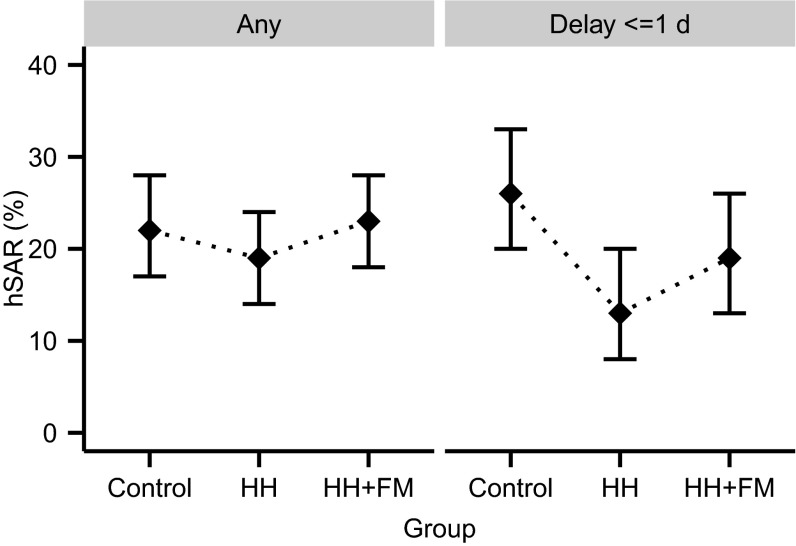
We analyze a superset of data from 322 households participating in a previously described known-index intervention study of influenza (7, 14). Three hundred and twenty-two of these were included in the primary analysis and randomly assigned to one of three groups: control (112 households), intervention with improved hand hygiene (HH, 106 households), or intervention with improved hand hygiene plus face masks (HH+FM, 104 households) (7). Each index case was initially screened by rapid test and confirmed using PCR. Nonindex household members were defined to be cases if they were PCR-confirmed on or after the second visit or if they showed at least two of the following signs and symptoms: temperature above 37.7 °C, cough, headache, sore throat, or myalgia (7, 19). Using traditional hSAR as the outcome for the primary analysis, a significant difference was observed between the control and HH arms, but only for a subset of households in which the index case attended clinic rapidly after the onset of symptoms (Fig. 1; see also Fig. S1) (7). Data from the 63 additional households included here could not be included in the primary analyses because either the index was not confirmed as infected by PCR (n = 16, despite being positive on rapid test) or because a household contact had RT-PCR-confirmed infection at the initial household visit (n = 47, defined to be coprimary) (7).

Fig. 1.

Proportions of household members meeting case criteria (using a composite definition based on symptoms and RT-PCR results) in different intervention groups and for different delay intervals between the time of symptom onset of index case and recruitment into the study. The 95% confidence intervals (CI) are represented by vertical bars. To aid direct comparison with previous work (7), these estimates excluded the 63 households in which the index patient did not have RT-PCR-confirmed infection or a household contact had RT-PCR-confirmed infection at the initial household visit.

Fig. S1.

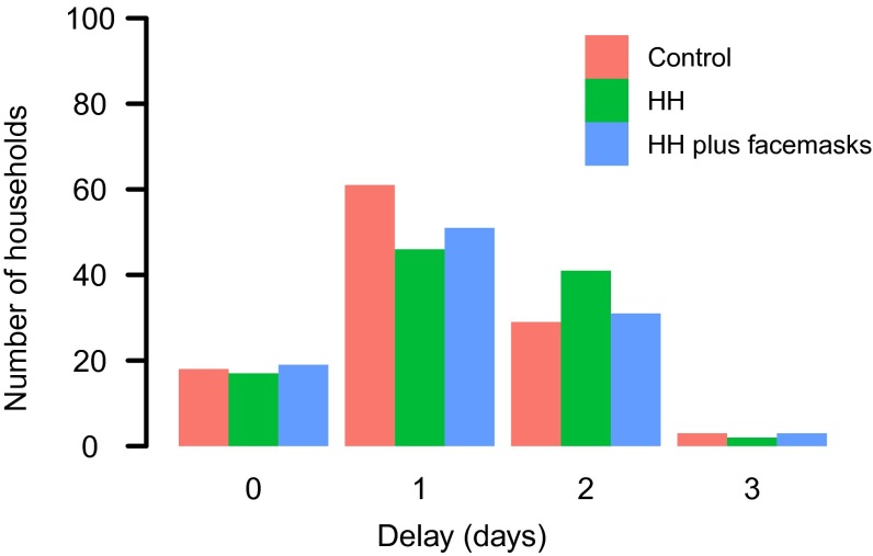
Number of households distributed over different delays between time of symptom onset of index cases and interventions.

Parameter Estimation and Validation.

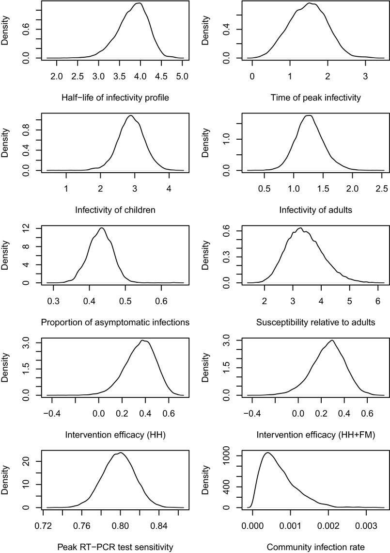
We defined a process model for the transmission of influenza in a study household, with parameters that would allow us to make inference on the efficacy of interventions and underlying dynamics (see Materials and Methods). We sampled from the joint posterior distribution of number of infections, times of infection, and process parameters of interest (Table 1), conditional on the full set of study results and uninformative prior distributions. The posterior distributions of model parameters are shown in Fig. S2. With the modal posterior values for the model parameters, we simulated study outcomes using the precise study protocol for each household and obtained distributions of hSAR consistent with the observed data (Tables S1 and S2). Also, for validation, we used multiple sets of these pseudodata to successfully reestimate the modal process parameters (Table S3).

Table 1.

Estimates of key model parameters

Parameters	Posterior mean [95% CI]
Half-life of the infectiousness profile, $a_{\text{eff}}$	3.86 [3.04, 4.43]
Time (day) of peak infectivity, b	1.50 [0.52, 2.42]
Infectivity of children per day, ${\beta }_1$	2.91 [2.13, 3.65]
Infectivity of adults per day, ${\beta }_2$	1.27 [0.83, 1.79]
Susceptibility of children relative to adults, ${\eta }_1$	3.36 [2.31, 4.82]
Peak level of RT-PCR test sensitivity, ψ	79.6% [76.5%, 83.0%]
Intervention efficacy per day for HH only, $r_2$	37.0% [8.3%, 57.8%]
Intervention efficacy per day for HH + FM, $r_3$	27.2% [-4.6%, 52.3%]

Fig. S2.

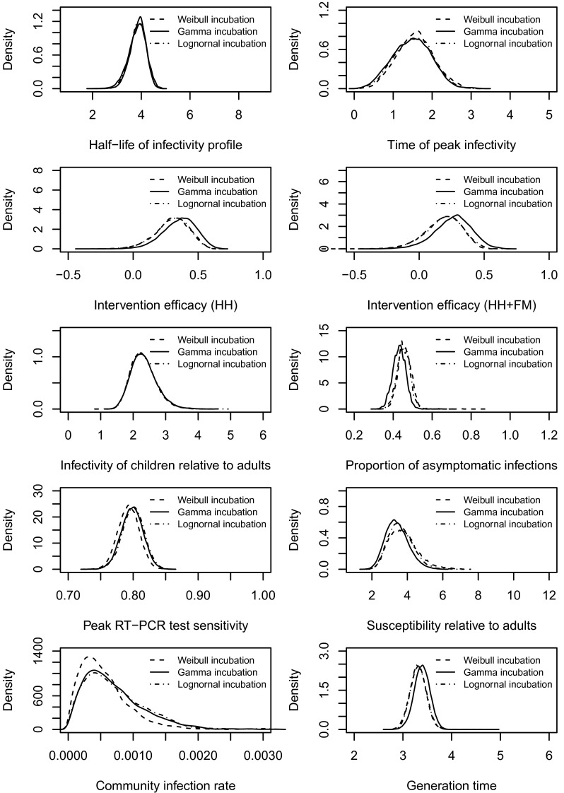
Posterior distributions of the model parameters. Note that we assumed $\mathit{ϵ}=0.8$ (see Infectiousness over time) and the test specificity $Q=0.99$. We have used uniform priors (see McMC Algorithm). Also see the summary of these distributions (Table 1) and other relevant comments in Results in the main text.

Table S1.

Summary of simulated observed hSAR for different household sizes from the estimated model (1,000 simulations)

Household size	hSAR, %
3	23.7 [17.9, 30.0] (24.2)
4	28.0 [23.1, 33.1] (31.1)
5	27.5 [22.4, 32.3] (27.1)

The mean values of the simulated observations are followed by 95% two-sided intervals (the observed values are shown in bold following the intervals. It is noticed that the observed hSAR lay within the 95% credible intervals obtained from the model simulated data, indicating a reasonably good fit of the model to the data (1, 2).

1. Cook AR, Otten W, Marion G, Gibson GJ, Gilligan CA (2007) Estimation of multiple transmission rates for epidemics in heterogeneous populations. Proc Natl Acad Sci USA 104(51):20392–20397.

2. Gibson GJ, et al. (2006) Bayesian estimation for percolation models of disease spread in plant populations. Stat Comput 16(4):391–402.

Table S2.

Summary of simulated observed hSAR for control and intervention groups from the estimated model (1,000 simulations)

	0 d delay, %	1 d delay, %	$\ge$ 2 d delay, %
hSAR (control)	24.1 [12.2, 36.04] (27.4)	24.3 [18.5, 31.0] (28.3)	26.5 [16.8, 36.3] (22.0)
hSAR (HH)	21.2 [9.6, 32.7] (26.3)	27.1 [20.1, 34.9] (27.9)	29.4 [21.7, 36.6] (31.0)
hSAR (HH+FM)	25.3 [13.8, 37.1] (21.0)	26.0 [18.5, 33.0] (29.1)	31.0 [23.3, 40.5] (31.5)

The mean values of the simulated observations are followed by 95% two-sided intervals (the observed values are shown in bold following the intervals). It is noticed that the observed hSAR lay within the 95% credible intervals obtained from the model simulated data, indicating a reasonably good fit of the model to the data (1, 2).

1. Cook AR, Otten W, Marion G, Gibson GJ, Gilligan CA (2007) Estimation of multiple transmission rates for epidemics in heterogeneous populations. Proc Natl Acad Sci USA 104(51):20392–20397.

2. Gibson GJ, et al. (2006) Bayesian estimation for percolation models of disease spread in plant populations. Stat Comput 16(4):391–402.

Table S3.

Summary of the posterior samples of model parameters from 10 simulations

Parameters	Posterior mean [95% CI]	True value
Relative infectivity of children to adults	2.52 [0.87, 10.29]	2.50
Relative susceptibility of children to adults	3.08 [0.97, 8.21]	3.0
Half-life of the infectiousness profile	4.08 [2.15, 5.44]	3.80
Time (day) of peak infectivity	1.80 [0.13, 4.43]	1.30
Proportion of asymptomatic infection	0.46 [0.21, 0.67]	0.40
Peak level of RT-PCR test sensitivity, %	72.9 [56.0, 92.8]	75.0
Intervention efficacy for HH only, %	28.3 [−19.0, 62.0]	29.0
Intervention efficacy for HH + FM, %	17.3 [−14.4, 61.1]	18.0

Note that as the community infection rate estimated from the data was insignificant, here we assumed it was known. The study design was preserved (e.g., the data structure in which the delay to interventions and the time of home visits were preserved). It was noticed that the posterior distributions appeared to be broadly consistent with the true values, which strengthened the validity of our algorithm.

Household Transmission Dynamics.

We estimated that, in this study, children were substantially more susceptible and infectious than were adults (Table 1). The infectiousness parameters for children and adults in the model are defined relative to the household size and are therefore somewhat difficult to assess directly. However, their ratio is easier to interpret, with children 2.29 [1.66. 3.23] times as infectious as adults and 3.36 [2.31, 4.82] times as susceptible. These results are broadly consistent with prior studies based only on symptomatic outcomes (2, 3, 20, 21).

The basic functional form of the infectiousness over time was assumed to be the log-normal density function truncated at day 10 (see Materials and Methods). Fig. 2A shows how the inferred amplitude of infectiousness varies over the time since infection for households of size 4. It was necessary to consider a specific household size because we assumed that pair-wise infectiousness between individuals could vary as a function of household size, i.e., as the size of the household increased, the probability of infection between each possible susceptible–infectious pair was not constant. These infectiousness profiles contrast somewhat with previous results (17) based only on symptoms. Although ref. 17 and our results both suggest that infectiousness is highest near the day of symptoms, our estimated profiles exhibit a fatter tail than that in ref. 17.

Fig. 2.

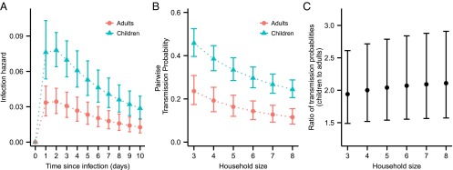
Infectivity profiles and pairwise transmission probabilities. (A) Estimated infectiousness over time, assuming household size 4 (median household size in data); vertical bars show 95% credible interval. (B) Estimated pairwise transmission probabilities for different household sizes. (C) Estimated pairwise transmission probabilities for children relative to adults.

To give a more intuitive description of the infectivity profiles, we also calculated the pairwise transmission probabilities (see SI Text, Pairwise transmission probability) of children and adults over the full period of their infectiousness, in the absence of interventions. Fig. 2 B and C shows the absolute and relative comparison between pairwise transmission probabilities of children and adults in different household sizes.

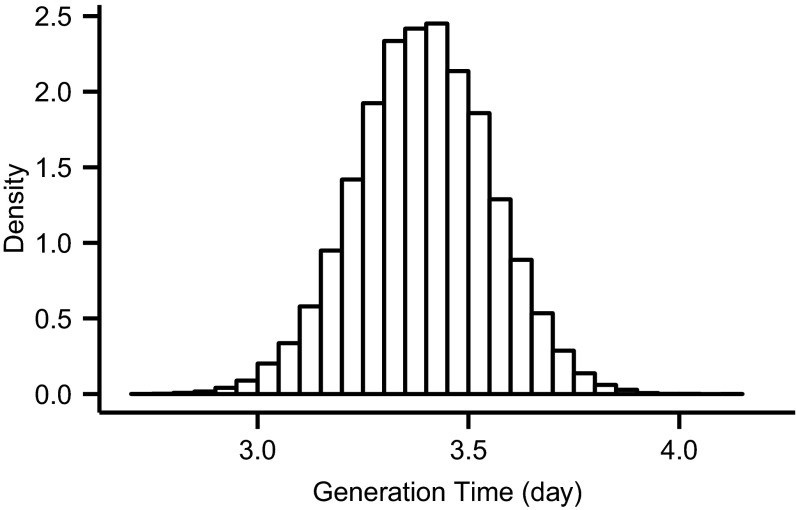
The generation time is defined as the expected delay between the infection of an infector and the infection of all their infectees across all infection types (22). Leveraging our ability to infer infection events, we were also able to estimate the approximate generation time commonly reported from household studies—the time between the infection of the index case and the infection of the secondary cases. We estimated this to be 3.39 d [3.06, 3.70] (Fig. S3), which was consistent with estimates in the literature for this and other strains of influenza A (23–25). This estimate was also somewhat sensitive to the ratio of the sensitivity of RT-PCR testing between asymptomatic infections and symptomatic infections (see Sensitivity Analysis).

Fig. S3.

Distribution of mean generation time.

Intervention Efficacy.

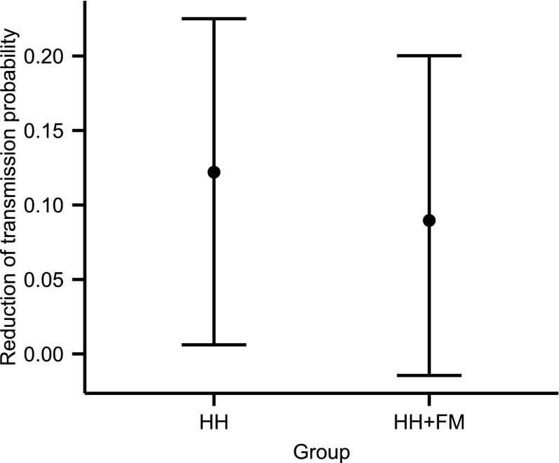
Intervention efficacy was modeled as the per day reduction of infectiousness and could take a different value in each of the three study arms. Using all available data, the efficacy in the HH group was estimated to be significantly different from 0 at 37.0% [8.3%, 57.8%] and, for HH+FM, was 27.2% [−4.6%, 52.3%] (Table 1). Although the reduction in infectivity was not significant for individual days, the cumulative effect reflected in the overall reduction in pairwise transmission probability was significant (Fig. 3).

Fig. 3.

Reduction of the pairwise transmission probability after interventions in the two different intervention arms (assuming household size 4).

By inferring the presence or absence of infections during the period of the study for all members of participating households (see Materials and Methods), we were able to compare the directly observed hSAR with an inferred hSAR. We estimated that only 61.7% [43.1%, 76.9%] of infections that occurred in households during the period of the study met the case criteria (see Study Data). This percentage was also somewhat sensitive to the ratio of the sensitivity of RT-PCR testing between asymptomatic infections and symptomatic infections (see Sensitivity Analysis). The underestimation was driven by variable timing of follow-up and also by variable sensitivity of the RT-PCR test, depending on the number of days since infection (26–28).

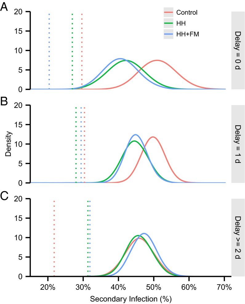
When the data were stratified by the delay between symptom onset in the index case and the interventions (i.e., the speed of intervention), the inferred hSARs described a more coherent story than the crude hSARs, with, in particular, higher numbers of infections being inferred in the control arm than would have been expected from the observed hSARs for delays of 2 d or greater (Fig. 4). Although the structural assumptions implicit in our model (see Discussion and Materials and Methods) must have constrained the inferred infection events to some degree, it is encouraging that the two interventions had similar efficacy for each delay strata and that the pattern of increasing efficacy with reducing delay was consistent. We also note that intervention efficacy was not defined to be positive definite (see SI Text), so the model had the flexibility to explore parameter regimes where interventions increased the risk of transmission. The differences between inferred and observed hSAR were likely driven by stochastic variation in the timing and frequency of follow-up between households.

Fig. 4.

Posterior densities of the rates of secondary infection in different study arms with different days of delay to intervention: (A) 0 d, (B) 1 d, and (C) 2 d. The distributions of the inferred hSAR (i.e., hSAR inferred from imputing the hidden infection process including the number of infections) are represented by solid curves. Dotted lines represent the hSAR based on original case criteria (i.e., the crude hSAR).

RT-PCR Test Sensitivity.

RT-PCR is the gold standard laboratory method for confirming viral respiratory infections among symptomatic individuals. We estimated the peak level of RT-PCR test sensitivity in this field study to be 79.6% [76.5%, 83.0%] for symptomatic infections. This estimate is fundamentally different from previous estimates because it incorporates uncertainty about the true state of the individual, as well as the performance of the sampling protocol and assay themselves. Although the relative sensitivity of asymptomatic infections was not identifiable in this analysis and was assumed to be half that of symptomatic infections (29), key model parameters appeared to be robust toward these assumptions (see Sensitivity Analysis).

Sensitivity Analysis.

We tested a number of our baseline assumptions and found few material differences in our results. In our baseline analyses, we assumed a Gamma distribution for the incubation period with mean 2 d and SD 0.2 d (30). Two alternative incubation periods were considered in the sensitivity analysis: a Weibull distribution with mean 1.48 d and SD 0.47 d (17) and a lognormal distribution with median 1.4 d and dispersion factor 1.51 d (31). These alternative assumptions for the incubation period produced results that were not materially different from the baseline results.

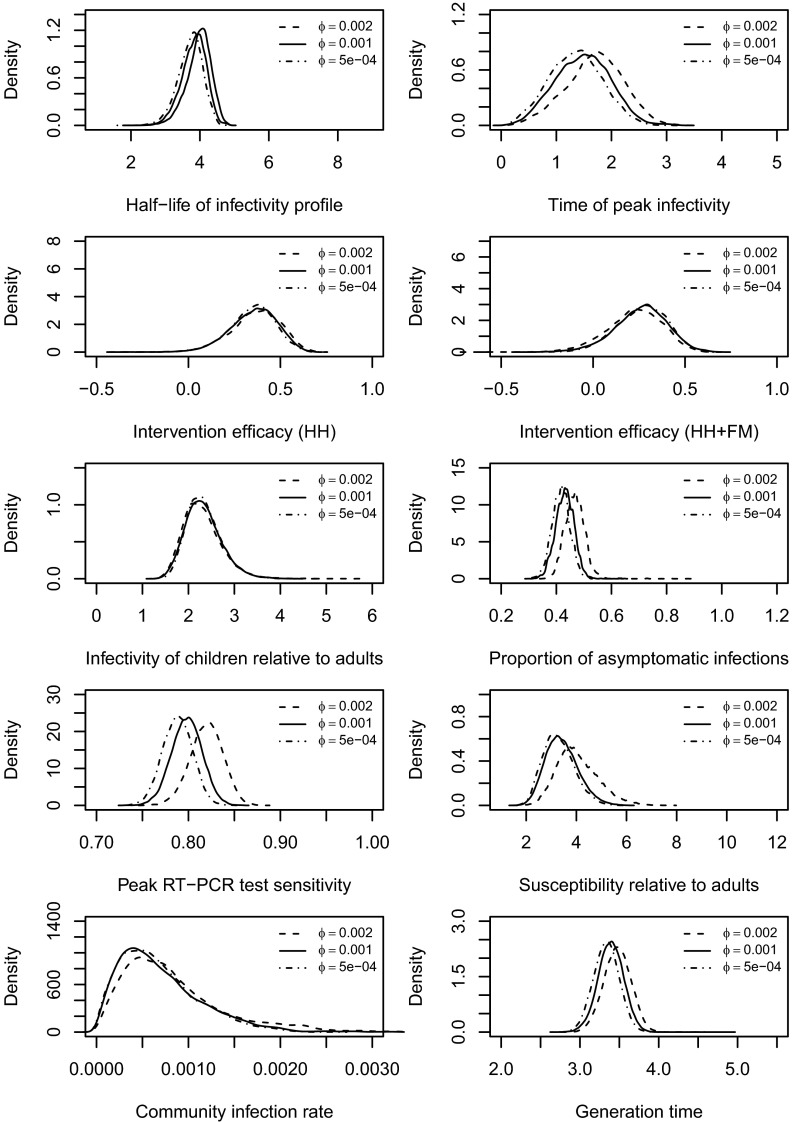
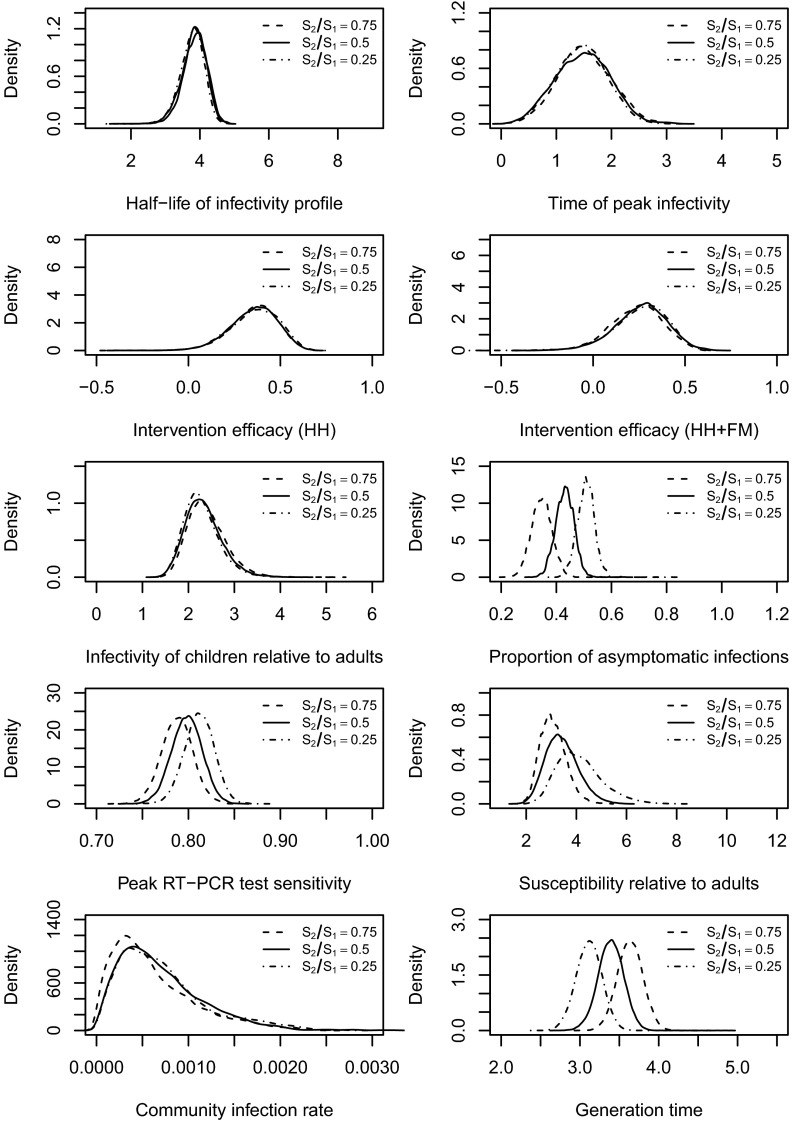
We also tested the robustness of assumptions about the ratio of the sensitivity of RT-PCR testing between asymptomatic infections and symptomatic infections, $S_2/S_1$. The value of this parameter ϕ (noninfection symptoms onset rate; see Materials and Methods) was assumed to be 0.001 in the baseline analysis (32, 33) and was varied in these sensitivity analyses. We tried a range of alternative values and found that higher values were associated with higher rates of asymptomatic infection. However, the values of other model parameters were not materially affected (see Figs. S4–S6).

Fig. S4.

Posterior distributions of the model parameters and the generation time by assuming different values of ϕ, the nuisance noninfection symptoms onset rate. In the baseline case, $\varphi =0.001$.

Fig. S6.

Posterior distributions of the model parameters and the generation time by assuming ratio of the sensitivity of RT-PCR testing between asymptomatic infections and symptomatic infections $S_2/S_1$. In the baseline case, $S_2/S_1=0.5$.

Fig. S5.

Posterior distributions of the model parameters and the generation time by assuming different incubation periods. A Gamma incubation period was used in the baseline case.

The distribution of the generation time (last panels in the Figs. S4–S6) and the distribution of the percentage of infections meeting case criteria (Table S4) were also somewhat sensitive to the assumed value of ratio of $S_2/S_1$. When the ratio $S_2/S_1$ changed from 0.25 to 0.75, the proportion of infections meeting cases criteria changed from 51% to 67%, and the mean of the generation time changed from 3.1 to 3.7. The values for the generation time remained within with the range suggested in the literature (23, 25).

Table S4.

Posterior distribution of the percentage of infections that met case criteria

Scenario	Posterior Mean, % [95% CI]
Base scenario	61.7 [43.1, 76.9]
$\varphi =0.002$	64.4 [44.0, 79.3]
$\varphi =0.0005$	61.5 [43.0, 75.5]
$S_2/S_1=0.75$	67.4 [47.8, 84.6]
$S_2/S_1=0.25$	56.1 [39.3, 69.8]
Weibull incubation	61.4 [43.0, 75.5]
Lognormal incubation	61.5 [43.1, 76.4]

Optimization of Study Design.

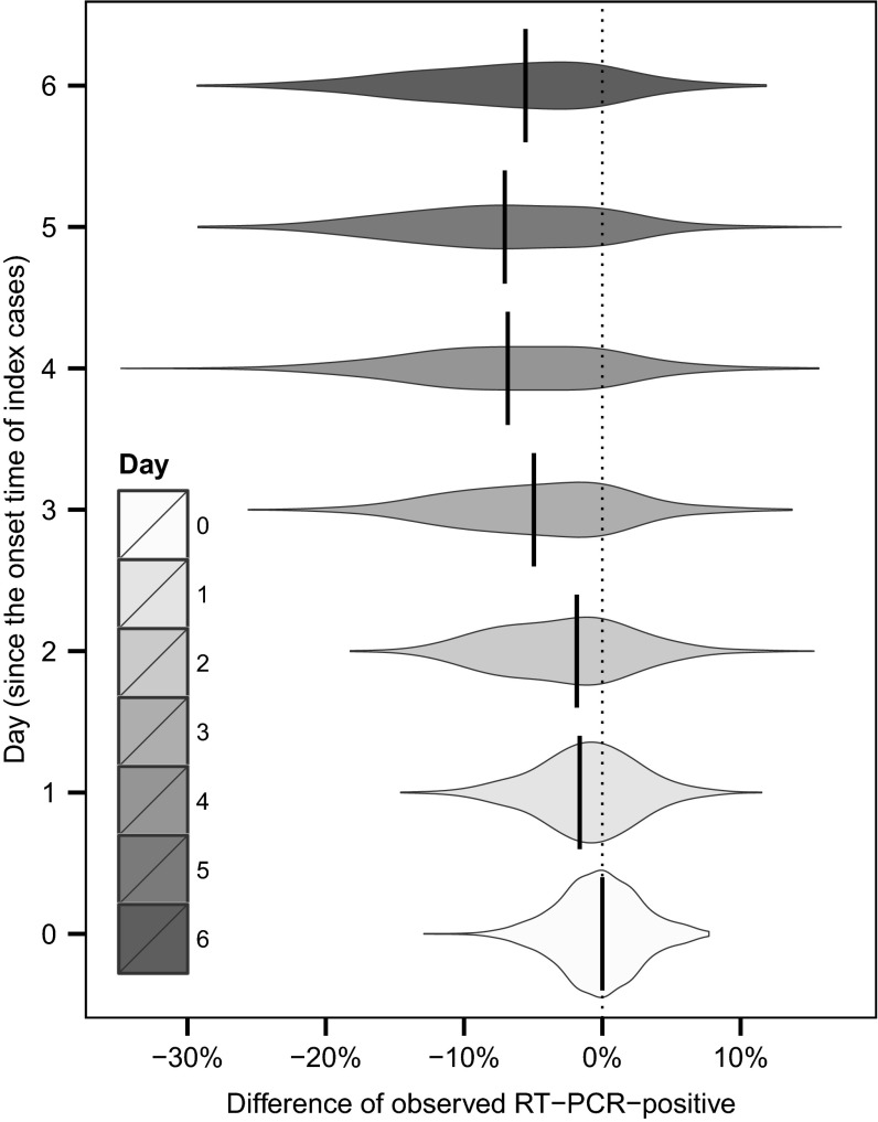
We used our estimated process model parameters to examine some specific issues around trial design. We designed a simulation experiment to explore how the timing of measurements (i.e., the timing of performing RT-PCR tests) may affect the outcome of the traditional analysis. Specifically, we answered the following question: If it was only possible to make a single visit to each household to evaluate an intervention (perhaps due to logistic constraints or cost-effectiveness considerations), what would be the best day to visit the household so that difference of number of infections (between intervention arms and control arm) may be more genuinely reflected by the traditional analysis? Based on the transmission-dynamic parameters estimated here, we simulated observations from our estimated model and assumed that only one home visit was carried out. To eliminate the effect due to the time of implementing the interventions, we only considered households with initial home visit within the same day as the symptoms onset of the index case. We found that a single sample at day 5 would have the highest expected difference in observed PCR-confirmed hSAR (Fig. 5). A single sample at day 4 would have a very similar expected difference between interventions and control but greater variance, suggesting that in day 4 or day 5 we may have the most “detectable” infections circulating in households.

Fig. 5.

Based on the transmission-dynamic parameters estimated here, we simulated observations from our estimated model and assumed that only one home visit was carried out. To eliminate the effect due to the time of implementing the interventions, we only considered households with initial home visit within the same day as the symptoms onset of the index case. We computed the simulated difference of RT-PCR-positive between HH group and control group. We considered seven scenarios in which the home visit was carried out, respectively, at day 0, day 1, day 2, day 3, day 4, day 5, and day 6 since the symptoms onset of the index cases.

Discussion

We incorporated both viral shedding data and symptomatic data into a transmission model that allowed the estimation of the efficacy of interventions and key epidemiological parameters. Our analysis refines the primary study analyses in estimating a significant effect in one intervention arm using data from all households, rather than data only from a (prespecified) subset, highlighting opportunities to improve on traditional measures such as the observed hSAR (7). We showed that intervention efficacy can be more accurately captured using a disease-dynamic model coupled with rigorous statistical inference. Also, by inferring the number and timing of infections, the underlying transmission dynamics could also be described and the impact of variable timing of interventions in household assessed. Subject to structural biases, we argue that this approach extracts substantial additional information from known-index transmission studies than does traditional analysis reliant on the hSAR. More generally, our results highlight the potential use of robust inference with well-designed mechanistic transmission models to improve the design of intervention studies.

Compared with other nonpharmaceutical interventions, such as quarantine and social distancing, the use of face masks and improved hand hygiene are simple and impose less burden on those infected and their contacts. Our results have helped to reinforce earlier findings of substantial efficacy. Also, we suggest that defining the estimated efficacy as a per-day reduction in transmission gives a more interpretable measure and could be a useful quantity to communicate as part of an overall health protection message.

Our study has a number of limitations associated with the structured assumptions implicit in our model. First of all, we only estimated the average efficacy of improved hand hygiene and face masks by aggregating other heterogeneities such as adherence and age distribution among the households. Nonetheless, adherence to hand hygiene intervention (i.e., the main contributing intervention in our study) was similar to that reported in previous community studies (34–36). Hence, although the estimated intervention efficacy should have varied with different adherence, the similarity of the adherence between our study and that in other community studies supports some generalization of our findings and the practicality of our conclusion.

We were not able to simultaneously estimate the reduction of absolute susceptibility and the reduction of infectivity due to interventions, as they were not identifiable with each other. Instead, to avoid this issue of identifiability, our model was parameterized by the relative susceptibility of children, and we estimated the reduction of infectivity. Children and adults were assumed to be subject to a common community infection rate, which may only represent a relatively crude average measure. However, as the study design aimed to recruit households that had infections mostly initiated by the index cases, the data may not be able to inform the community infection at a finer resolution. Nevertheless, the estimated common community infection rate appeared to be insignificant and hence was believed not have a significant impact (see Fig. S3).

A parallel analysis of these data using a different approach found evidence suggesting that aerosol (small droplets) transmission might be responsible for approximately half of all influenza transmission in households (37). Our results are consistent with this finding, because only a small to medium effect of face masks and hand hygiene would be expected given that they are thought to reduce transmission via large droplets and contact. Further extensions of our modeling framework could be considered in the future to account for different modes of transmission.

Although there is some evidence that children might have a higher level and a longer duration of shedding (23, 38) compared with adults, we assumed the same underlying function. Also, we only estimated the sensitivity of RT-PCR as a function of time since infection, and it was assumed to peak between 2 d and 5 d after infection (i.e., around the mean time of symptoms onset) (39). A more direct factor affecting the test sensitivity may be the viral shedding (26–28). Future work in linking viral shedding explicitly with the test sensitivity could further refine the approach we have used here.

Our framework can be used to answer specific questions related to trial design as well as to conduct secondary analysis of existing data. Here, we illustrated this by estimating the best possible day for a single follow-up visit in an interventions trial. However, a more systematic trial design study with well-defined resources that may be constrained may well produce far more efficient protocols, perhaps varying by household size and age distribution.

Materials and Methods

Details of Data Collection.

In 2008, from 2 January through 30 September, 407 index patients with influenza-like illness with symptom onset in the previous 48 h, and who were positive for influenza A or B virus by QuickVue Influenza A$\mathrm{+}$ B rapid testing, were recruited at outpatient clinics in Hong Kong. Households with fewer than two members or those with members reporting influenza-like illness in the preceding 14 d were excluded. There were, in total, 322 eligible households who agreed to participate. The households were randomly assigned to one of the three groups: control group ($n=112$ households), intervention group with improved hand hygiene ($n=106$) and intervention group with face masks and improved hand hygiene ($n=104$). The intervention was carried out in an initial home visit scheduled within 2 d after the randomization. Demographic data and nasal and throat swab specimens from all household members who were 2 y of age or older were collected during the home visit. All household contacts were required to keep daily symptom diaries within the observational period after the initial intervention. Further nasal and throat swab specimens from all household members were collected in subsequent home visits, which were scheduled usually around 3 d and 6 d after the initial visit. More details on the study design can be found in a previous paper (7).

Transmission Model.

We developed a stochastic model to jointly capture the study design, the transmission process, and the efficacy of the interventions. Household members were classified by their ages (i.e., children and adults) and were otherwise identical.

There were four major components to be explicitly modeled: (unobserved) infection times, symptom onset times, RT-PCR test results, and the intervention efficacy. Here, we describe the assumed processes related to each of these components. Each infected member was assumed to exhibit time-varying infectivity (i.e., hazard of infection) since infection, which was parameterized by its median a and mode b. Specifically, we used a log-normal density function truncated at day 10 to represent this infectivity profile; we denoted the effective median (i.e., half-life) of the infectivity profile after truncation as $a_{\text{eff}}$. Children and adults were assumed to have different scaling factors ${\beta }_i$ to the infectivity profile (${\beta }_1$ and ${\beta }_2$ for children and adults, respectively). We also assumed children were ${\mathit{\eta }}_1$ times more susceptible than adults. A coefficient ε was used to explain the dependency between the infectiousness and household size. Consequently, the hazard of infection $H_{k\to j}\left(t\right)$ exerted on a susceptible member j by an infected member k was determined by coupling the infectivity profile with the household size and the age and time since infection of member k. The total hazard of infection exerted on member j at time t in the household was then taken to be the aggregated hazard of infection $H\left(t\right)$ from other infected members at time t in the household, i.e.,

$$H\left(t\right)={\displaystyle \sum _{k\ne j}^n{H}_{k\to j}\left(t\right)}.$$ [1]

We allowed a constant community infection hazard ρ common to children and adults on top of the within-household hazard. Interventions were assumed to reduce the magnitude of the infectivity profile by a constant proportion $r_i$, where $i=\mathrm{1,2,3}$ corresponded to the control, HH and HH+FM arms, respectively; because we were interested in the efficacy of HH and HH+FM arms relative to the control arm, we set $r_1=0$. Interventions had no effect on the community infection.

A nonindex case has a probability p to be an asymptomatic infection. Given the infection time, onset time of a symptomatic case was determined by an assumed incubation period parameterized by α and γ. Also, for the robustness of the model, we had ϕ as a nuisance parameter representing the background constant rate of noninfection symptoms onset (32, 33). The RT-PCR testing results were assumed to depend on times of measurements, a (peak) test sensitivity ψ, and a test specificity Q. The test sensitivity was assumed to be a (step) function of the time since infection and to peak around the mean of the incubation period (also see SI Text for details). The test sensitivity of asymptomatic infections was assumed to be half that of symptomatic infections (see also different assumed values used in Sensitivity Analysis). Lastly, households were assumed to be independent given the sparse recruitment.

Events above were also described mathematically in SI Text.

Bayesian Inference and McMC.

Let $\mathit{\theta }$ be the parameter vector containing the model parameters described in Transmission Model. Estimation for the model parameters was performed in the Bayesian framework (i.e., we estimated the parameters from the posterior distributions for the parameters). Denoting the observed data by $\mathbf{x}$ and the joint likelihood for all households by $L\left(\mathit{\theta };\mathbf{x}\right)$, the posterior distribution of parameters given $\mathbf{x}$ was $P\left(\mathit{\theta }|\mathbf{x}\right)\propto L\left(\mathit{\theta };\mathbf{x}\right)\pi \left(\mathit{\theta }\right)$, where $\pi \left(\mathit{\theta }\right)$ was the assumed prior distribution for $\mathit{\theta }$. We used marginal noninformative uniform priors for individual parameters in $\mathit{\theta }$ (i.e., $\pi \left({\theta }_i\right)\approx U\left(c,d\right)$, where c and d represented conservative lower and upper bound of ${\theta }_i$). Markov chain Monte Carlo techniques (40) were applied to obtain the posterior distribution, i.e., we constructed the Markov chain in such a way that the stationary distribution was the posterior distribution $P\left(\mathit{\theta }|\mathbf{x}\right)$ of interest. Details of the construction of the likelihood function and of the McMC algorithm are given in SI Text.

Hidden Infection Process.

Symptom onset and RT-PCR are not perfect indicators for an infection [e.g., the symptom onset might have a different etiology, and the sensitivity of RT-PCR is only high at the time of peak infectiousness (26–28)]. To handle this uncertainty and to capture more accurately the underlying transmission dynamics, we required an algorithm that allows proper probabilistic transitions of a household member between the status of infected and noninfected. Specifically, we applied a reversible jump algorithm (41, 42) in which deletion (i.e., transit from infected to noninfected) and addition (i.e., transit from noninfected to infected) of an infection is allowed. More details on the inference of times on infection and how the process parameters and infection times were updated in the same algorithm are given in SI Text.

SI Text

Definition of Events and Likelihood Function.

Within each household, we denoted ${\mathbf{t}}^I\mathrm{=}\left(t_1^I\mathrm{,}{t}_2^I\mathrm{,\dots ,}{t}_n^I\right)$ and ${\mathbf{t}}^O\mathrm{=}\left(t_1^O\mathrm{,}{t}_2^O\mathrm{,\dots ,}{t}_n^O\right)$ as the vectors containing the infection times and time of symptoms onset, respectively, of the members in a household, where n was the total number of household members; ${\mathbf{t}}^P\mathrm{=}\left(t_1^P\mathrm{,}{t}_2^P\mathrm{,\dots ,}{t}_m^P\right)$ was the vector containing the testing times of the household, which was common for all household members in the household. In all of the vectors just defined, the first entry corresponded to the quantity for the index case. Also, we had ${\mathbf{p}}_j\mathrm{=}\left(p_{j,1}\mathrm{,}{p}_{j,2}\mathrm{,\dots ,}{p}_{j,m}\right)$ containing the test results for individual j in the household, where m is the total number of times the test was carried out and the index case corresponds to $j\mathrm{=}1$; $p_{j,k}\in \left\{\mathrm{1,0}\right\}$, $k\mathrm{=}1\mathrm{,}2\mathrm{,\dots ,}m$, where 1 and 0 represented a positive result and negative result, respectively. Lastly, we denoted ${\mathbf{R}}_{m\times n}$ as the data matrix storing the test results of all household members (i.e., the jth column of ${\mathbf{R}}_{m\times n}$ was ${\mathbf{p}}_j$). All times of different events were scaled such that the day of intervention was equal to day zero.

Because we assumed households were independent, we present likelihood for one household in this section. The joint likelihood for all households is straightforward after specifying the likelihood for a single household. Denoting ${\mathbf{t}}_{-1}^I$ and ${\mathbf{t}}_{-1}^P$ as the vectors excluding the first entries of ${\mathbf{t}}^I$ and ${\mathbf{t}}^P$, respectively, we can write down the likelihood function for a household j as

$$L_j\left(\mathit{\theta };\mathbf{R},{\mathbf{t}}_{-1}^I,{\mathbf{t}}_{-1}^O,t_1^I,t_1^O\right)={\displaystyle \prod _{j=2}^n{f}_j\left(t_j^I\right)}\times {\displaystyle \prod _{j=2}^n{g}_j\left(t_j^O\right)}\times {\displaystyle \prod _{j=1}^n{h}_j\left({\mathbf{p}}_j\right)}\times W\left(t_1^O-t_1^I|\alpha ,\gamma \right)$$ [S1]

where the parameters defined in Transmission Model in the main text were $\mathit{\theta }=\left({\beta }_1,{\beta }_2,{\eta }_1,\mathit{ϵ},r_2,r_3,\psi ,Q,a,b,\alpha ,\gamma ,\rho ,\varphi \right)$. The factors in Eq. S1 corresponded to likelihood contribution of infection events, symptoms onset times, RT-PCR test results, and the infection times of index cases, respectively. In the remainder of this section, detailed definition of these events and their exact mathematical representations are given.

Infectiousness over time.

We assumed that the infectiousness of an infectee varied according to the time since infection. Any infected person in the household contributed a hazard of infection, determined by a function

$$\frac{{\beta }_i}{n^{\mathit{ϵ}}}\times {\lambda }_I\left(\tau \right),$$ [S2]

to other susceptible members in the household, where τ, ${\beta }_i(i=\mathrm{1,2})$, n, and ε were the time since infection, the infectiousness parameter (it corresponded to the children when i = 1 and to the adults when i = 2), the household size, and the coefficient that explained the dependency between the infectiousness and household size, respectively [we assumed $\mathit{ϵ}=0.8$ (1, 2)]. For mathematical convenience, we specified ${\lambda }_I\left(\tau \right)$ to be a proper density function. The lognormal density function $K\left(\tau |a,b\right)$ with two parameters a and b was used, where a and b were median and mode, respectively, of the lognormal density function. We truncated this function at day 10 since infection; given the 7-d follow-up in the study (i.e., started from the first home visit for the household, normally 7 d follow up was given in which subsequent home visits were arranged and symptoms data were collected), we should not expect that we can estimate reliably the infectiousness at later days (e.g., 10 d) since infection. Note that a is merely a nominal half-life of the infectivity profile as we truncated the profile at day 10; we reported the (effective) half-life corresponding to the truncated profile $a_{eff}$(see Table 1 and Fig. S3). We also allowed a community hazard of infection ρ.

Relative susceptibility and intervention efficacy.

It was assumed that the infectiousness per day was reduced by a constant proportion equal to the intervention efficacy since the day of intervention applied. It should be noted that because the variation of adherence was not modeled, the interventions efficacies in our model represented average daily efficacies by aggregating the adherence.

Denote $A\left(t\right)$ as the total force of infection from other household members to a particular individual j after taking into account of the interventions. We had

$$A\left(t\right)={\eta }_j\times H\left(t\right)\times \left(\mathbf{1}\left\{t\ge t_v\right\}\times e^{v_i}+\mathbf{1}\left\{t<t_v\right\}\right)$$ [S3]

where $H\left(t\right)$ was the hazard of infection exerted on individual j at time t in the household and was taken to be the aggregated hazard of infection from other infected members at time t in the household, i.e.,

$$H\left(t\right)={\displaystyle \sum _{k\ne j}^n{H}_{k\to j}\left(t\right)},$$ [S4]

where $H_{k\to j}\left(t\right)$ was the hazard exerted by k at j determined by coupling the infectivity profile with the age of individuals k and j (i.e., the heterogeneity of infectivity among different age groups), household size, and the time since infection of individual k (see also Eq. S2 and Materials and Methods).

As a result, the conditional probability that individual j (excluding the index case) got infection at day T given the infection times of all other members was

$$f_j\left(T\right)=\left(1-exp\left(-(A\left(T\right)+\rho \right)\right)\times exp\left(-{\displaystyle \sum _{-14\le t\le T-1}\left(A\left(t\right)+\rho \right)}\right)$$ [S5]

where ρ was the constant community hazard of infection. Also, $\mathbf{1}\{.\}$, $t_v$ were the indicator function and day intervention started, respectively; ${\eta }_j$ reflected the susceptibilities in different ages groups (j = 1 for children; j = 2 for adults). We set ${\eta }_2$ equal to 1 so we were only estimating the susceptibility of children relative to adults. Also, $v_i$ $\left(i=\mathrm{1,2,3}\right)$ related to the interventions efficacies ($v_1$ related to the efficacy of the control group and was set to be $log\left(1\right)$, and $v_2$ and $v_3$ related to the efficacy for the hand hygiene group and hand hygiene plus face masks group, respectively. The corresponding percentage of reduction of infectiousness was $1-e^{v_i}$. For notational convenience, we used $r_i$ to represent $1-e^{v_i}$. It should be noted that setting the intervention efficacy of the control arm to be 0 (i.e., $1-e^{log\left(1\right)}$) guaranteed that our estimates for $r_2$ and $r_3$ were the efficacies relative to the control arm.

If individual j was an noninfectee, $f_i\left(T\right)$ reduced to

$$exp\left(-{\displaystyle \sum _{-14\le t\le t_{max}}\left(A\left(t\right)+\rho \right)}\right)$$

where $t_{max}$ was the follow-up period (see Missing Data) for the household.

In the majority of recruiting sites, the criterion for recruitment was a positive result for influenza A or B using the QuickVue rapid diagnostic test on a nose and throat swab. Therefore, it can be safely assumed that the index case was an infectee, and the distribution of infection time can be determined from the reported symptoms onset time together with an assumed distribution of the incubation period (i.e., the difference between time of infection and time of symptoms onset). See the last product in Eq. S1.

Pairwise transmission probability.

The integration of the infectiousness profile ${\displaystyle {\int }_{-\infty }^T\left({\beta }_i/n^{\mathit{ϵ}}\right)\times {\lambda }_I\left(\tau \right)d\tau }$ represented an aggregate risk of infection, and we can derive the pairwise probability of getting infection q up to day T from the expression $exp\left\{-{\displaystyle {\int }_{-\infty }^T\left({\beta }_i/n^{\mathit{ϵ}}\right)\times {\lambda }_I\left(\tau \right)d\tau }\right\}=1-q$.

Symptoms onset.

We defined acute respiratory infection as follows: at least 2 symptoms out of fever (temperature ≥37.8 °C), cough, headache, sore throat, and myalgia (3, 4). Similar to the event of infection, we assumed that the hazard of having the symptoms onset of an infected person follows a function of time since infection, denoted as ${\lambda }_s\left(\tau \right)$. Also, we used a nuisance parameter ϕ to allow noninfection symptoms onset (5, 6).

Relation between hazard and incubation period.

Symptoms onset ${\lambda }_s\left(\tau \right)$ was closely related to the incubation period. Denoting $W\left(\tau |\alpha ,\gamma \right)$ as the incubation period distribution, which was assumed to be a two-parameter density function (a discretized gamma distribution was used), the relationship between the hazard function and the incubation period was as follows:

$$W\left(\tau |\alpha ,\gamma \right)=\left(1-exp\left(-{\lambda }_s\left(\tau \right)\right)\right)\times exp\left(-{\displaystyle \sum _{t\le \tau -1}{\lambda }_s\left(t\right)}\right).$$ [S6]

Therefore, given the incubation period, the hazard function for symptoms onset ${\lambda }_s\left(\tau \right)$ can be computed iteratively starting from $\tau =1$. We assumed a Gamma incubation period distribution with mean 2 d and SD 0.25 d (7).

Asymptomatic infection.

The conversion between the incubation period distribution and hazard function was only valid if the infected case was certain for having symptoms onset, but this was not always the case. Therefore, we introduced a parameter, p, to indicate the probability that a case was an asymptomatic infection.

As a result, the probability for an infected individual j to have symptoms onset at day $T\ge t_j^I$, where $t_j^I$ is the infection time of the individual j, therefore was equal to

$$g_j\left(T\right)=exp\left(-{\displaystyle \sum _{-14\le t\le t_j^I-1}\varphi }\right)\times \{\left(1-p\right)\times \left(1-exp\left(-\left({\lambda }_s\left(T-t_j^I\right)+\varphi \right)\right)\right)\times \left(exp\left(-{\displaystyle \sum _{t_j^I\le t\le T-1}\left({\lambda }_s\left(t-t_j^I\right)+\varphi \right)}\right)\right)+p\times \left(1-exp\left(-\varphi \right)\right)\times \left(exp\left(-{\displaystyle \sum _{t_j^I\le t\le T-1}\varphi }\right)\right)\}\mathrm{\cdot }$$ [S7]

Also, if the infected individual j had no reported symptoms onset, $g_j\left(T\right)$ reduced to

$$exp\left(-{\displaystyle \sum _{-14\le t\le t_j^I-1}\varphi }\right)\times \left\{\left(1-p\right)\times exp\left(-{\displaystyle \sum _{t_j^I\le t\le t_{max}}\left({\lambda }_s\left(T-t_j^I\right)+\varphi \right)}\right)+p\times exp\left(-{\displaystyle \sum _{t_j^I\le t\le t_{max}}\varphi }\right)\right\}.$$

The respective probabilities for the case with $T<t_j^I$ and for symptoms onset of noninfected individuals were straightforward to write down by disregarding the contribution of ${\lambda }_s(\cdot )$.

RT-PCR test results.

RT-PCR was used for confirmation of infection. The symptoms onset and infection times characterized the complete transmission process. The testing data were conditionally independent of the transmission process but provided additional information for the inference of the transmission process.

One of the key elements in correctly incorporating the test results was the adoption of appropriate values of the sensitivity and specificity for the RT-PCR test. The test was, in general, of high sensitivity and specificity (8, 9). However, the sensitivity of the RT-PCR test was correlated to the time since infection and the viral load (10–13). We assumed a constant specificity 0.99 and estimated the sensitivity at disjoint time intervals since infection. Specifically, we had the sensitivity over the time since infection $\mathrm{\Delta }t$,

$$S\left(\mathrm{\Delta }t\right)=\{\begin{array}{ll}\psi /3,\hfill & \text{for}\hspace{0.17em}0\le \mathrm{\Delta }t\le 2.\hfill \\ \psi ,\hfill & \text{for}\hspace{0.17em}2\le \mathrm{\Delta }t\le 5.\hfill \\ \psi /3,\hfill & \text{for}\hspace{0.17em}5\le \mathrm{\Delta }t\le 10.\hfill \\ 0,\hfill & \text{otherwise}.\hfill \end{array}$$ [S8]

Note that the infectiousness may typically die out after 10 d since infection (also, given our 7-d follow-up period, we may not expect that we are able to estimate the sensitivity after 10 d since infection).

Denoting $q_j^{+}\left(t_k^p\right)$ and $q_j^{-}\left(t_k^p\right)$ as the probabilities of individual j having positive and negative test results, respectively, from kth test at the testing day $t_k^p$, we had

$$q_j^{+}\left(t_k^p\right)=\mathbf{1}\left\{\left(\frac{{\beta }_i}{n^{\mathit{ϵ}}}\lambda \left(t_k^p-t_j^I\right)\times \left(\mathbf{1}\left\{t_k^p\ge t_v\right\}\times e^{v_i}+\mathbf{1}\left\{t_k^p<t_v\right\}\right)\right))>0\right\}\mathrm{\times }S\left(t_k^p\mathrm{-}{t}_j^I\right)+\mathbf{1}\left\{\left(\frac{{\beta }_i}{n^{\mathit{ϵ}}}\lambda \left(t_k^p-t_j^I\right)\times \left(\mathbf{1}\left\{t_k^p\ge t_v\right\}\times e^{v_i}+\mathbf{1}\left\{t_k^p<t_v\right\}\right)\right))\le 0\right\}\mathrm{\times }\left(1\mathrm{-}Q\right)$$

and

$$q_j^{-}\left(t_k^p\right)=1-q_j^{+}\left(t_k^p\right)$$

where $S\left(t\right)$, $Q=0.99$ were the functions governing the sensitivity and the specificity of the RT-PCR test, respectively.

Therefore, we had the probability of observing the test results, ${\mathbf{p}}_j$, for the individual j

$$h_j\left({\mathbf{p}}_j\right)={\displaystyle \prod _{k=1}^m\left(\mathbf{1}\left\{p_{i,k}=1\right\}\times q_j^{+}\left(t_k^p\right)+\mathbf{1}\left\}{p}_{i,k}=0\right\}\times q_j^{-}\left(t_k^p\right)\right)}.$$ [S9]

Missing Data.

In the symptoms diaries collected, we found incomplete records. Also, the collection of specimens for RT-PCR was not complete. The missing patterns in both data were not regular. For example, within a household, we might find that one of the household members had an entry missing only on one particular day during the 7-d follow-up period but other members had the complete record. This induced extra difficulty in setting up a fixed timeframe for the transmission process. Therefore, herein we used a minimally complete approach such that we truncated the data of the symptoms record up to the point where every member in the household had complete records. This was equivalent to shortening the study period of a particular household with incomplete records to avoid the missing data issue. About 12% of the households had the data truncated, and the mean of the number of days of data truncated was 2 d. Because the RT-PCR testing was a conditionally independent process from the transmission, we could easily discard the missing records. Also, the records of RT-PCR test results that were obtained beyond the fixed timeframe determined by the symptoms record were discarded to retain the consistency.

McMC Algorithm.

The objective of the McMC sampling was to simulate from the joint posterior distribution of model parameters and the unobserved data, which can be represented as

$$\pi \left(\mathit{\theta },\mathit{z}|\mathit{y}\right)\propto L\left(\mathit{\theta };\mathit{z}\right)\pi \left(\mathit{\theta }\right),$$ [S10]

where $\mathit{y}$ was the observed data, $\mathit{z}$ represented the complete data, and $\pi \left(\mathit{\theta }\right)$ represented the prior distribution of model quantities.

The inference of the parameters in the model was challenging mainly due to the presence of unobserved infection process, and the specification of the likelihood function depends on the correct distinction between infectee and noninfectee. However, symptom onset and RT-PCR were not perfect indicators for an infection [e.g., the symptom onset might have a different etiology, and the sensitivity of RT-PCR is only high at the time of peak infectiousness (10–13)]. To handle this uncertainty and to capture more accurately the underlying transmission dynamics, we required an algorithm that allows proper probabilistic transitions of a household member between the status of infected and noninfected. Specifically, we required the ability to apply a reversible jump algorithm (14, 15) in which deletion (i.e., transit from infected to noninfected) and addition (i.e., transit from noninfected to infected) of an infection is allowed.

First, we performed a single-component Metropolis–Hastings algorithm (16) to sample the model parameters that include a, b, ${\beta }_1$, ${\beta }_2$, ${\eta }_1$, ρ, ψ, p, $v_2$, and $v_3$. The unknown infection times were also sampled. At each iteration, the algorithm sampled different components in the following sequence: (i) the infection times of nonindex cases; (ii) the infection times of the index cases; (iii) a and b, the median and mode parameter of the infectiousness profile; (iv)${\beta }_1$, ${\beta }_2$, ${\eta }_1$, ρ, ψ, p, $v_2$, and $v_3$; and (v) apply a reversible jump algorithm in which one infection is added or deleted from the population.

Moves i and ii were performed in each household, and the samples were pooled. Without the concern of the distinction between infected and noninfected, a conventional algorithm was to randomly choose an infectee and then uniformly sample an infection time from the support, i.e., the infection time would be drawn from $U\left[-14,t_{max}\right]$ in our case, where $t_{max}$ corresponded to the duration of study period for the particular household since the day of intervention and $-14$ was chosen to give a reasonable lower bound of the infection time relative to onset time. Adapted from ref. 15, we implemented a deletion and an addition of an infection.

Move ii was carried out in a manner similar to that in move i. As the index case was assumed to be infected, there was no distinction problem. At each iteration, a new infection time was proposed by drawing from $U\left[-14,t_1^O\right]$, and the acceptance was determined similarly to move i. Move iii and move iv followed random walk Metropolis–Hastings algorithm in which symmetric proposal densities were used.

We used noninformative uniform priors for individual parameters with reasonably specified lower and upper bounds. Specifically, we had $U\left(\mathrm{0,10}\right)$ for a and b. We had $U\left(-\infty ,+\infty \right)$ for $v_2$ and $v_3$ (which allowed negative intervention efficacies). Also, we had $U\left(\mathrm{0,1}\right)$ for p and ψ, as they were probabilities. Finally, we had $U\left(0,+\infty \right)$ as priors for other model parameters.

References

- 1.Cowling BJ, et al. Comparative epidemiology of pandemic and seasonal influenza A in households. N Engl J Med. 2010;362(23):2175–2184. doi: 10.1056/NEJMoa0911530. [DOI] [PMC free article] [PubMed] [Google Scholar]
- 2.Cauchemez S, et al. Household transmission of 2009 pandemic influenza A (H1N1) virus in the United States. N Engl J Med. 2009;361(27):2619–2627. doi: 10.1056/NEJMoa0905498. [DOI] [PMC free article] [PubMed] [Google Scholar]
- 3.Cauchemez S, Carrat F, Viboud C, Valleron AJ, Boëlle PY. A Bayesian MCMC approach to study transmission of influenza: Application to household longitudinal data. Stat Med. 2004;23(22):3469–3487. doi: 10.1002/sim.1912. [DOI] [PubMed] [Google Scholar]
- 4.Longini IM, Jr, Koopman JS, Monto AS, Fox JP. Estimating household and community transmission parameters for influenza. Am J Epidemiol. 1982;115(5):736–751. doi: 10.1093/oxfordjournals.aje.a113356. [DOI] [PubMed] [Google Scholar]
- 5.Longini IM, Jr, Koopman JS, Haber M, Cotsonis GA. Statistical inference for infectious diseases. Risk-specific household and community transmission parameters. Am J Epidemiol. 1988;128(4):845–859. doi: 10.1093/oxfordjournals.aje.a115038. [DOI] [PubMed] [Google Scholar]
- 6.Wu JT, Riley S, Fraser C, Leung GM. Reducing the impact of the next influenza pandemic using household-based public health interventions. PLoS Med. 2006;3(9):e361. doi: 10.1371/journal.pmed.0030361. [DOI] [PMC free article] [PubMed] [Google Scholar]
- 7.Cowling BJ, et al. Facemasks and hand hygiene to prevent influenza transmission in households: A cluster randomized trial. Ann Intern Med. 2009;151(7):437–446. doi: 10.7326/0003-4819-151-7-200910060-00142. [DOI] [PubMed] [Google Scholar]
- 8.MacIntyre CR, et al. Face mask use and control of respiratory virus transmission in households. Emerg Infect Dis. 2009;15(2):233–241. doi: 10.3201/eid1502.081167. [DOI] [PMC free article] [PubMed] [Google Scholar]
- 9.Canini L, et al. Surgical mask to prevent influenza transmission in households: A cluster randomized trial. PLoS ONE. 2010;5(11):e13998. doi: 10.1371/journal.pone.0013998. [DOI] [PMC free article] [PubMed] [Google Scholar]
- 10.Halloran ME, Hayden FG, Yang Y, Longini IMJ, Jr, Monto AS. Antiviral effects on influenza viral transmission and pathogenicity: Observations from household-based trials. Am J Epidemiol. 2007;165(2):212–221. doi: 10.1093/aje/kwj362. [DOI] [PubMed] [Google Scholar]
- 11.Longini IMJ, Jr, Halloran ME, Nizam A, Yang Y. Containing pandemic influenza with antiviral agents. Am J Epidemiol. 2004;159(7):623–633. doi: 10.1093/aje/kwh092. [DOI] [PubMed] [Google Scholar]
- 12.Esposito S, et al. Effectiveness of influenza vaccination of children with recurrent respiratory tract infections in reducing respiratory-related morbidity within the households. Vaccine. 2003;21(23):3162–3168. doi: 10.1016/s0264-410x(03)00253-6. [DOI] [PubMed] [Google Scholar]
- 13.Hurwitz ES, et al. Effectiveness of influenza vaccination of day care children in reducing influenza-related morbidity among household contacts. JAMA. 2000;284(13):1677–1682. doi: 10.1001/jama.284.13.1677. [DOI] [PubMed] [Google Scholar]
- 14.Cheng CK, et al. Factors affecting QuickVue Influenza A + B rapid test performance in the community setting. Diagn Microbiol Infect Dis. 2009;65(1):35–41. doi: 10.1016/j.diagmicrobio.2009.05.003. [DOI] [PubMed] [Google Scholar]
- 15.Lambert SB, et al. Comparing nose-throat swabs and nasopharyngeal aspirates collected from children with symptoms for respiratory virus identification using real-time polymerase chain reaction. Pediatrics. 2008;122(3):e615–e620. doi: 10.1542/peds.2008-0691. [DOI] [PubMed] [Google Scholar]
- 16.Wrammert J, et al. Broadly cross-reactive antibodies dominate the human B cell response against 2009 pandemic H1N1 influenza virus infection. J Exp Med. 2011;208(1):181–193. doi: 10.1084/jem.20101352. [DOI] [PMC free article] [PubMed] [Google Scholar]
- 17.Ferguson NM, et al. Strategies for containing an emerging influenza pandemic in Southeast Asia. Nature. 2005;437(7056):209–214. doi: 10.1038/nature04017. [DOI] [PubMed] [Google Scholar]
- 18.Papenburg J, et al. Household transmission of the 2009 pandemic A/H1N1 influenza virus: Elevated laboratory‐confirmed secondary attack rates and evidence of asymptomatic infections. Clin Infect Dis. 2010;51(9):1033–1041. doi: 10.1086/656582. [DOI] [PubMed] [Google Scholar]
- 19.Monto AS, et al. Zanamivir prophylaxis: An effective strategy for the prevention of influenza types A and B within households. J Infect Dis. 2002;186(11):1582–1588. doi: 10.1086/345722. [DOI] [PubMed] [Google Scholar]
- 20.Rampey AH, Jr, Longini IM, Jr, Haber M, Monto AS. A discrete-time model for the statistical analysis of infectious disease incidence data. Biometrics. 1992;48(1):117–128. [PubMed] [Google Scholar]
- 21.Bell D, et al. World Health Organization Writing Group Non-pharmaceutical interventions for pandemic influenza, national and community measures. Emerg Infect Dis. 2006;12(1):88–94. doi: 10.3201/eid1201.051371. [DOI] [PMC free article] [PubMed] [Google Scholar]
- 22.Wallinga J, Lipsitch M. How generation intervals shape the relationship between growth rates and reproductive numbers. Proc Biol Sci. 2007;274(1609):599–604. doi: 10.1098/rspb.2006.3754. [DOI] [PMC free article] [PubMed] [Google Scholar]
- 23.Carrat F, et al. Time lines of infection and disease in human influenza: A review of volunteer challenge studies. Am J Epidemiol. 2008;167(7):775–785. doi: 10.1093/aje/kwm375. [DOI] [PubMed] [Google Scholar]
- 24.Ferguson NM, et al. Strategies for mitigating an influenza pandemic. Nature. 2006;442(7101):448–452. doi: 10.1038/nature04795. [DOI] [PMC free article] [PubMed] [Google Scholar]
- 25.Cowling BJ, Fang VJ, Riley S, Malik Peiris JS, Leung GM. Estimation of the serial interval of influenza. Epidemiology. 2009;20(3):344–347. doi: 10.1097/EDE.0b013e31819d1092. [DOI] [PMC free article] [PubMed] [Google Scholar]
- 26.Cheng PK, et al. Performance of laboratory diagnostics for the detection of influenza A(H1N1)v virus as correlated with the time after symptom onset and viral load. J Clin Virol. 2010;47(2):182–185. doi: 10.1016/j.jcv.2009.11.022. [DOI] [PubMed] [Google Scholar]
- 27.Lee N, et al. Viral loads and duration of viral shedding in adult patients hospitalized with influenza. J Infect Dis. 2009;200(4):492–500. doi: 10.1086/600383. [DOI] [PMC free article] [PubMed] [Google Scholar]
- 28.Poon LL, et al. Early diagnosis of SARS coronavirus infection by real time RT-PCR. J Clin Virol. 2003;28(3):233–238. doi: 10.1016/j.jcv.2003.08.004. [DOI] [PMC free article] [PubMed] [Google Scholar]
- 29.Lau LL, et al. Viral shedding and clinical illness in naturally acquired influenza virus infections. J Infect Dis. 2010;201(10):1509–1516. doi: 10.1086/652241. [DOI] [PMC free article] [PubMed] [Google Scholar]
- 30.Ghani A, et al. The early transmission dynamics of H1N1pdm influenza in the United Kingdom. PLoS Curr. 2009;1:RRN1130. doi: 10.1371/currents.RRN1130. [DOI] [PMC free article] [PubMed] [Google Scholar]
- 31.Lessler J, et al. Incubation periods of acute respiratory viral infections: A systematic review. Lancet Infect Dis. 2009;9(5):291–300. doi: 10.1016/S1473-3099(09)70069-6. [DOI] [PMC free article] [PubMed] [Google Scholar]
- 32.Birrell PJ, et al. Bayesian modeling to unmask and predict influenza A/H1N1pdm dynamics in London. Proc Natl Acad Sci USA. 2011;108(45):18238–18243. doi: 10.1073/pnas.1103002108. [DOI] [PMC free article] [PubMed] [Google Scholar]
- 33.Hadler JL, et al. Case fatality rates based on population estimates of influenza-like illness due to novel H1N1 influenza: New York City, May-June 2009. PLoS ONE. 2010;5(7):e11677. doi: 10.1371/journal.pone.0011677. [DOI] [PMC free article] [PubMed] [Google Scholar]
- 34.Sandora TJ, et al. A randomized, controlled trial of a multifaceted intervention including alcohol-based hand sanitizer and hand-hygiene education to reduce illness transmission in the home. Pediatrics. 2005;116(3):587–594. doi: 10.1542/peds.2005-0199. [DOI] [PubMed] [Google Scholar]
- 35.Luby SP, et al. Effect of handwashing on child health: A randomised controlled trial. Lancet. 2005;366(9481):225–233. doi: 10.1016/S0140-6736(05)66912-7. [DOI] [PubMed] [Google Scholar]
- 36.Luby SP, et al. Combining drinking water treatment and hand washing for diarrhoea prevention, a cluster randomised controlled trial. Trop Med Int Health. 2006;11(4):479–489. doi: 10.1111/j.1365-3156.2006.01592.x. [DOI] [PubMed] [Google Scholar]
- 37.Cowling BJ, et al. Aerosol transmission is an important mode of influenza A virus spread. Nat Commun. 2013;4:1935. doi: 10.1038/ncomms2922. [DOI] [PMC free article] [PubMed] [Google Scholar]
- 38.Sato M, Hosoya M, Kato K, Suzuki H. Viral shedding in children with influenza virus infections treated with neuraminidase inhibitors. Pediatr Infect Dis J. 2005;24(10):931–932. doi: 10.1097/01.inf.0000180976.81055.ce. [DOI] [PubMed] [Google Scholar]
- 39.Klick B, Leung GM, Cowling BJ. Optimal design of studies of influenza transmission in households. I: Case-ascertained studies. Epidemiol Infect. 2012;140(1):106–114. doi: 10.1017/S0950268811000392. [DOI] [PMC free article] [PubMed] [Google Scholar]
- 40.Chib S, Greenberg E. Understanding the Metropolis–Hastings algorithm. Am Stat. 1995;49(4):327–335. [Google Scholar]
- 41.Green PJ. Reversible jump Markov chain Monte Carlo computation and Bayesian model determination. Biometrika. 1995;82(4):711–732. [Google Scholar]
- 42.Gibson GJ, Renshaw E. Estimating parameters in stochastic compartmental models using Markov chain methods. IMA J Math Appl Med Biol. 1998;15:19–40. [Google Scholar]