Principles of Use of Biostatistics in Research

Abstract

Collecting, analyzing, and interpreting data are essential components of biomedical research and require biostatistics. Doing various statistical tests has been made easy by sophisticated computer software. It is important for the investigator and the interpreting clinician to understand the basics of biostatistics for two reasons. The first is to choose the right statistical test for the computer to perform based on the nature of data derived from one’s own research. The second is to understand if an analysis was performed appropriately during review and interpretation of others’ research. This article reviews the choice of an appropriate parametric or nonparametric statistical test based on type of variable and distribution of data. Evaluation of diagnostic tests is covered with illustrations and tables.

Educational Gap

A basic understanding of biostatistics is needed to understand and interpret the medical literature.

Objective

After completing this article, the readers should be able to:

• Improve understanding of principles of biostatistics pertaining to neonatal research.

Introduction

The American Board of Pediatrics revised the content outline for neonatal-perinatal medicine subspecialty in 2010. Core knowledge in scholarly activities accounts for 7% of all questions in the boards. This section includes the following subsections:

1. Principles of use of biostatistics in research

2. Principles of epidemiology and clinical research design

3. Applying research to clinical practice

4. Principles of teaching and learning

5. Ethics in research

This article provides a brief overview of biostatistics in research and covers all the topics except systematic reviews and meta-analysis (to be covered in a subsequent article on epidemiology and clinical research design) required by the American Board of Pediatrics content outline. The reader is referred to other board review and biostatistics books listed under suggested reading for a complete understanding of biostatistics. (1)(2)(3)(4)(5)

A requirement to understand many statistical principles and answer questions is creation of a basic table (Table 1). If a test accurately identifies the disease, it is true-positive. If a test accurately identifies absence of a disease, it is called true-negative. By convention, disease is on the top row and test is on the first column.

Table 1.

Basic Statistics Table

Disease	Disease Present	Disease Not Present
Test positive	True-positive	False-positive
Test negative	False-negative	True-negative

Study 1

The neonatal faculty at the regional perinatal center decided to evaluate the association between formula feeding in preterm infants and necrotizing enterocolitis (NEC). Pre-term neonates (gestational age <34 weeks at birth) are followed during their NICU course for NEC. Those who developed NEC were classified into stage I, stage II, and stage III and compared with infants who were not diagnosed with NEC during their NICU course. Infants fed exclusively with human milk were compared with infants fed preterm formula (Fig 1).

Figure 1.

Description of commonly used variables in a study evaluating the association of formula feeds with necrotizing enterocolitis (NEC) in preterm infants.

1. Types of Variables

Any characteristic that can be observed, measured, or categorized is called a variable. It is important to distinguish different types of variables:

1. Categorical: Not suitable for quantification; classified into categories.

   1. Nominal: Named categories, with no implied value (for example, blood groups: although group A and group O are different categories, one blood group is not “superior” or “greater” than another). Another example is types of truncus arteriosus (type I, type II, type III). The numbers serve as labels and many arithmetic operations on these numbers do not make sense. So, a nominal variable is existential; it exists or does not exist and has no inherent order or superiority (Fig 2). Nominal data with only two groups are referred to as dichotomous or binary (eg, male or female).

   2. Ordinal: Named with an order/ superiority; stages of NEC: stage III is worse than stage II and stage II is worse than stage I. However, having an episode of stage III NEC is not three times worse than an episode of stage I NEC. Ordinal variables have an order but the magnitude of difference between these orders is not considered (Figs 1 and 2). Many arithmetic operations do not make sense when they are applied to ordinal data.

2. Continuous: A variable that can have an infinite number of possible values.

   1. Interval: Equal interval between values but no meaningful zero point (eg, infant’s body temperature in °F; the difference between 98.4°F and 97.4°F is the same as the difference between 99.4°F and 98.4°F. However, 0°F does not mean that there is no temperature).

   2. Ratio: Equal intervals with a meaningful zero point and all mathematical operations are functional. For example, a nasogastric tube was placed in an infant with NEC and placed on continuous suction. The volume of gastric aspirate is quantified in milliliters per day. If a baby has 15 mL nasogastric drainage per day, it is quantitatively three times higher than having 5 mL drainage per day. If the drainage is 0 mL over a 24-hour period, it means that there was no nasogastric drainage. Similarly, enteral intake of human milk or formula expressed as milliliters per kilogram per day is a ratio variable.

3. To summarize, remember the mnemonic NOIR (Fig 2):

   1. Nominal variable has no implied value or order

   2. Ordinal variable has an order but not at equal intervals

   3. Interval variable has equal intervals but no meaningful zero

   4. Ratio variable has equal intervals with a meaningful zero

Figure 2.

Common types of variables and choosing the appropriate statistical test for these variables.

How Does the Type of Variable Affect the Choice of Statistical Test?

Statistical tests that assume that the population from which the data are sampled to be normally distributed (or approximately so) are known as “parametric” tests. Normal distribution (see below) of the population is essential for these tests to be valid. If the data do not conform to a normal distribution, “nonparametric” tests should be used.

Parametric tests can be used with interval and ratio data but not with nominal or ordinal data. In contrast, nonparametric tests can be used with any type of variable, including nominal or ordinal data (Fig 2).

Variables are also classified as the dependent variable (outcome of interest, which should change in response to some intervention, eg, diagnosis of NEC) or the independent variable (intervention or what is being manipulated, eg, providing donor human milk versus formula feeds). The appropriate simple statistical test based on the type of independent and dependent variables is shown in Table 2.

Table 2.

Choosing Simple Statistical Tests Based on the Type of Variable (Assuming Normal Distribution for Continuous Variables)

Independent Variable	Dependent Variable
	Dichotomous	Continuous (normal distribution)	Continuous (distribution is not normal)
Dichotomous	χ2 (large numbers) or Fisher’s exact test (small numbers)	t test (2 groups) or ANOVA (for more than 2 groups)	Nonparametric tests Wilcoxon rank sum test Kruskal-Wallis test
Continuous	t test or ANOVA	Pearson’s correlation coefficient	Spearman’s rank correlation coefficient

ANOVA=analysis of variance.

Study 2

Twenty-five preterm infants on mechanical ventilation received varying doses of hydrocortisone for 9 days in an attempt to achieve extubation. Baseline blood pressure was measured before hydrocortisone therapy and daily during therapy. Blood pressure was measured in 50 age-matched infants who did not receive hydrocortisone. Hypertension was defined as systolic blood pressure above 90th percentile for postmenstrual age. Based on Table 2 and assuming that blood pressure and hydrocortisone dose are normally distributed, the choice of statistical test is as follows:

• Classify patients into hydrocortisone treated and not treated and hypertensive and not hypertensive (two dichotomous categorical variables): χ² test

• Compare change in mean blood pressure from baseline and compare hydrocortisone versus no hydrocortisone: t test

• Compare cumulative dose of hydrocortisone (mg/kg) to change in systolic blood pressure from baseline (two continuous variables): correlation

2. Distribution of Data

Distribution of data includes measures of central tendency, dispersion, and distribution.

1. Central tendency: Estimates the “center” of the distribution

   1. MEAN

      1. The mean is the sum of all observations divided by the number of observations.

      2. The mean is the measure of central tendency for interval and ratio data and is the “average” value for the data.

      3. It is representative of all data points and is the most efficient estimator of the middle of a normal (Gaussian) distribution; however, it is inappropriate as a measure of central tendency if data are skewed.

      4. The mean is influenced by outlying values, particularly in small samples.

      5. Mean is commonly used for interval and ratio data.

   2. MEDIAN

      1. The median is that value such that half of the data points fall above it and half below it. It is the middle value when data are sequentially ordered from lowest to highest or highest to lowest.

      2. It is not influenced by outlying values and is more appropriate for data that are not normally distributed (skewed data).

      3. Median is also commonly used for ordinal data (eg, Apgar score).

   3. MODE

      1. Mode is the most frequently occurring observation.

      2. It is particularly useful while describing data distributed in a bimodal pattern when mean and median are not appropriate. For example, nosocomial infections in the NICU have a bimodal gestational age at birth distribution. Extremely preterm infants with percutaneous lines and full-term infants with surgical procedures are at risk. The mean or median age of these infants with nosocomial infections may be 34 weeks and is not representative of the central tendency in this population.

      3. Mode is commonly used with nominal data (eg, commonest maternal blood group associated with neonatal hyperbilirubinemia).

2. Distribution:

   1. NORMAL

      1. Also known as Gaussian distribution, and refers to a symmetric bell-shaped frequency distribution, in which mean, median, and mode all have the same value (Fig 3A).

      2. Kurtosis refers to how flat or peaked the curve is. for example, in Fig 3A, curve B is a normal distribution (excess kurtosis ~0, also called mesokurtic); curve A is peaked (excess kurtosis >0, also known as leptokurtic) compared with curve B and curve C is “flatter” with a lower central peak and broader (excess kurtosis <0, also known as platykurtic). All the three curves are symmetric and have the same mean, median, and mode values.

      3. An appropriate statistical test would be a parametric test such as a t-test or an analysis of variance (ANOVA).

      4. Data are usually represented as mean (SD).

   2. SKEWED

      1. In Fig 3B, curves D and E are skewed.

      2. The terminology for skewness can be confusing. Curve D is said to be skewed right or has a positive skew. Curve E is skewed left or has a negative skew. The direction of the skew refers to the direction of the tail, not to where the bulk of the data are located.

      3. An appropriate statistical test would be a non-parametric test, such as Wilcoxon test or Mann-Whitney test.

      4. Data are usually represented as median, inter-quartile range (IQR).

3. Measures of dispersion: A measure of dispersion refers to how close the data cluster around the measure of central tendency.

   1. RANGE is the difference between the highest and the lowest values. Range can change drastically when the study is repeated. It is also dependent on sample size (range widens if more subjects are added) and is influenced by extreme values.

   2. INTERQUARTILE RANGE (IQR) is the range between the 25th and 75th percentiles or the difference between the medians of the lower half and upper half of the data and comprises the middle 50% of the data. IQR is less influenced by extreme values and is represented in a box plot.

   3. VARIANCE is a measure of dispersion or average deviation from the mean. It is the sum of the square of the deviation from the central value.

   4. STANDARD DEVIATION (SD) is the square root of variance and is the most common measure of dispersion used for normally distributed data. For a normal distribution, if the mean and SD are known, the percentage of the sample included in a given range of values can be calculated.

      1. Mean ± 1 SD: 68.2% of the sample is included

      2. Mean ± 2 SDs: 95.4% of the sample is included

      3. Mean ± 3 SDs: 99.8% of the sample is included

   5. The STANDARD ERROR OF MEAN (SEM) is calculated by dividing the SD by the square root of n. It is the SD of the error in the sample mean relative to the true mean of the total population. With increasing sample size (n), SEM decreases.

      1. The SD reflects how close individual scores cluster around the sample mean, whereas the SEM shows how close mean scores from repeated random samples will be to the true population mean.

      2. With increasing size of a random sample, the mean of the sample comes closer to the population mean.

Figure 3.

A. Types of symmetric curves with different levels of kurtosis (peak or flatness). As the curves are normally distributed and symmetric, the mean, median, and mode values are the same. B. Skewed curves (D and E): Curve D has a positive skew or is skewed right and curve E has a negative skew or is skewed left. Note that the values for mode, median, and mean are different with a skewed distribution.

3. Hypothesis Testing

Let us review study 1 and Fig 1. This study has the following elements:

• Sample: Preterm infants in the NICU

• Predictor variable: Feeding

• Outcome variable: NEC

A simple hypothesis has one predictor and one outcome variable. For example, preterm infants who are exclusively fed human milk have a lower incidence of NEC is a simple hypothesis.

A complex hypothesis has more than one predictor variable. Preterm infants with maternal chorioamnionitis and exposure to indomethacin for patent ductus arteriosus (PDA) and formula feeds have a higher incidence of NEC is a complex hypothesis.

1. Null hypothesis refers to restating the research hypothesis to one that proposes no difference between groups being compared. The statement that “there is no difference in the incidence of NEC in preterm infants fed human milk compared with preterm infants fed formula” is a null hypothesis.

2. An alternative hypothesis proposes an association. Preterm infants who are exclusively fed human milk have a lower incidence of NEC is an alternative hypothesis.

1. An alternative hypothesis is either one-sided (only one direction of association will be tested) or two-sided (both directions will be tested).

   1. Preterm infants fed human milk have a lower incidence of NEC compared with formula-fed preterm infants is an example of a one-sided hypothesis.

   2. Preterm infants fed human milk have a different incidence of NEC compared with formula-fed preterm infants (increased risk or decreased risk) is an example of a two-sided hypothesis.

2. One-sided hypotheses should be used only in unusual circumstances, when only one direction of the association is clinically or biologically meaningful. This is rarely used. For example, the use of vancomycin for late-onset sepsis is associated with a higher risk of red-man syndrome than placebo. It is highly unlikely that placebo use will have a higher incidence of red-man syndrome than vancomycin.

3. Switching from a two-sided to a one-sided alternative hypothesis to reduce the P value is not appropriate.

4. Statistical Tests

4A. Parametric Tests

These tests assume the underlying population to be normally distributed and are based on means and SDs: the parameters of a normal distribution.

• (a)t test

  1. Student’s t test is a simple, commonly used parametric test to compare two groups of continuous variables that are normally distributed.

  2. The t test compares the means of two groups and is based on the ratio of the difference between groups to the SE of the difference.

  3. “Paired” t test: Each patient/subject serves as his/her own control before and after an intervention. For example, Fig 4 comparing birth-weight and weight at 10 days after birth in a group of preterm infants. This test accounts for systematic variance between subjects.

  4. “Unpaired” t test: Two groups of patients/subjects are compared with each other. For example, Fig 4 comparing human milk–fed and formula-fed infants and comparing weight gain over the first 10 days after birth.

  5. One-tailed hypothesis: Only one direction of association will be tested. For example, assuming that weight at 10 days after birth will be greater than birthweight.

  6. Two-tailed hypothesis: Both directions of association will be tested. For example, weight may increase or decrease over the first 10 days after birth in preterm infants; for practical purposes, most t tests performed in neonatal research should be two-tailed, with rare exceptions.

• (b)Analysis of Variance (ANOVA)

  1. One-way ANOVA is an extension of the two-sample t test to three or more samples and deals with statistical test on more than two groups (eg, weight gain over the first 10 days after birth is compared among mother’s expressed milk–fed, donor milk–fed, and formula-fed preterm infants).

  2. The sum of squares representing the differences between individual group means and a second sum of squares representing variation within groups are analyzed.

  3. Other methods, such as planned or post hoc comparisons, are conducted to examine specific comparisons among individual means.

     1. Planned comparisons are hypotheses specified before the analysis commences. Before the commencement of the study, it is hypothesized that weight gain over the first 10 days after birth is compared among small for gestational age, appropriate for gestational age, and large for gestational age will not be different and this analysis is planned.

     2. Post hoc comparisons are for further exploration of the data after a significant effect has been found. This analysis is occurring out of interest after the primary analysis has rejected the null hypothesis. For example, formula-fed infants gain more weight during the first 10 days after birth compared with mother’s or donor milk–fed infants. The investigator now wonders if increased weight gain with formula is observed only in infants who are small for gestational age and conducts a post hoc analysis.

  4. Factorial ANOVA performs complex analysis involving multiple independent factors. Additional information is derived from the interaction between factors.

  5. ANOVA repeated measures examines multiple (more than two) measures per subject that may be a result of more than one factor (eg, birth-weight is compared with weight at 10, 20, 30, and 40 days after birth and weight at discharge among breast-fed, donor milk–fed, and formula-fed preterm infants).

Figure 4.

Paired and unpaired t test. Paired test compares the same patient/subject before and after an intervention (nutrition and weight). Each individual subject is compared with himself/herself. Two groups of patients are compared in an unpaired t test (weight gain in human milk–fed and formula-fed preterm infants).

4B. Nonparametric Tests Make No Assumption About the Population Distribution

• (c)Wilcoxon rank test/Mann-Whitney U test are used to compare ordinal data. Human milk–fed and formula-fed preterm infants are compared based on the stage of NEC (Stage 0=no NEC, Stage I=nonspecific signs, Stage II=pneumatosis, and Stage III=intestinal perforation). These tests also can be used to analyze interval or ratio data that are not normally distributed.
• (d)Other tests that are not commonly used are listed in Fig 5 and readers are referred to books mentioned under suggested reading for more information on these tests.

Figure 5.

Choosing the right statistical test. Some of the tests described in this flow diagram are not described in the text. The reader is referred to a textbook of biostatistics for a detailed description of these statistical tests.

Other Commonly Used Statistical Tests

• (e)χ² test (Chi-squared test)

  1. The χ² test is a common test used to compare categorical data. Data are first entered into a 2 × 2 contingency table. Table 3 compares nominal or dichotomous variables: type of feeds and presence or absence of NEC. This test compares the proportion of disease (NEC) in one group (human milk feeds) versus another (formula feeds). Significance is calculated by analyzing the square of observed values and expected values.

  2. If the numbers are small (expected value is ≤5), an alternative test called Fisher’s exact test is used.

Table 3.

Association Between Feeds and NEC

Disease → Exposure ↓	Disease (NEC) Present	Disease (NEC) Not Present	Total
Exposure to formula present (formula feeds)	5 (a)	45 (b)	50 (a + b)
No exposure to formula (human milk feeds)	1 (c)	49 (d)	50 (c + d)
Total	6 (a + c)	94 (b + d)	100 (a + b + c + d)

A 2 × 2 contingency table. NEC=necrotizing enterocolitis.

4C. Interpretation of P Value

Table 4 explains type I and type II errors during interpretation of a statistical test.

Table 4.

Type I and Type II Errors

True Condition (In the Population)
Trial study results	Therapies are different	Therapies are not different
Therapies are different	True positive (correct decision)	False-positive (type I error) Probability = α (same as P value)
Therapies are not different	False-negative (type II error) Probability = β	True-negative (correct decision)

Normally, α is 5% or 0.05 (setting a P value) and power is (1 − β), often, 0.8 or 0.9 (80% or 90% power). P value and power are used in sample size calculations.

1. TYPE I ERROR (false-positive, also known as a rejection error) is rejection of a null hypothesis that is actually true in the population. The investigator concludes that there is a significant difference between the groups when, in fact, there is no true difference. This risk can be reduced by setting a more stringent P value (eg, .01 instead of .05).

2. TYPE II ERROR (false-negative, also known as an acceptance error) is failure to reject a null hypothesis that is actually false. The investigator concludes that there is no difference when a difference actually exists in the population. Increasing the sample size will reduce the risk of these errors.

3. P VALUE is the probability of the null hypothesis being true by chance alone. It is also the probability of committing a type I error. A P value of .05 or less is commonly used to denote significance. This value informs the investigator that there is at least a 95% chance that the two samples represent different populations.

   1. A lower P value (<.01) indicates a lower likelihood (1%) that the null hypothesis may be true due to chance alone.

   2. A lower P value does not infer a higher strength of association or clinical importance of an association.

   3. Factors that tend to decrease P value and increase significance are increased sample size, increased difference in control and experimental means, and less variance (low SD) (Fig 6A).

   4. Factors that tend to increase P value and decrease significance are small sample size, small difference between control and experimental means, and high variance/SD (Fig 6B).

   5. Interpreting P value when multiple comparisons have been made: When multiple comparisons are made, why not just do a bunch of t tests? If the probability of making a type I error on any one comparison is set at .05, it is important to recognize that a more stringent P value should be set if multiple comparisons are being performed (approximately, the P value is set at .05 ÷ the number of comparisons performed). This is called a Bonferroni correction.

4. CONFIDENCE INTERVAL

   1. There are approximately 4 million births in the United States every year. Your hospital has 4,000 deliveries per year. Using all the births at your hospital as your sample (sample size = 4,000), you intend to estimate the mean birth-weight of all infants born in the United States. The sample mean from your hospital very likely will not be identical to the population mean.

      1. The range of values that you expect to include the actual mean of the true population is referred to as the confidence interval (Fig 7).

      2. The values at either extreme of this range are called confidence limits.

      3. The probability of including the population mean within the confidence interval is the level of confidence, typically 95% confidence intervals are used in research. A higher level of confidence (99%) will widen the range of the confidence interval.

      4. 95% confidence interval is sample mean ± 1.96 SEM. As mentioned earlier, SEM = SD/√n, where n is the sample size. A 99% confidence interval is sample mean ± 2.58 SEM (and hence a wider confidence interval compared with the 95% confidence interval).

      5. Based on this equation, larger sample size (n), and smaller SD will narrow the confidence interval.

   2. When expressing relative risk or odds ratio (OR), 95% or 99% confidence limits are mentioned. The interpretation of these confidence intervals is described in the next section.

Figure 6.

Factors influencing P values. A large sample size, increased numeric difference between the means and less variability within the groups will reduce P value and increase statistical significance (A). A small sample size, small numeric difference between the means, and increased variability within the groups will increase P value and reduce statistical significance (B). This hypothetical example is comparing placebo (control group) and hydrocortisone (experimental group) for extubation of patients at risk for bronchopulmonary dysplasia and comparing diastolic blood pressure, as mentioned in study 2.

Figure 7.

Confidence interval. The true population mean (birthweight in this example) is shown by the black circle. The white circle represents the mean of a small sample (eg, your hospital deliveries). The 95% confidence interval is shown by the solid line (and is mean ± 1.96 × SEM). Increasing confidence from 95% to 99% will widen the range of the confidence interval to mean ± 2.58 × SEM). Increasing the sample size (eg, including all births in a county or state) will narrow the confidence interval.

5. Measures of Association

Table 3 demonstrates the association between formula and human milk feeds with NEC. The probability of developing NEC in formula-fed preterm infants is a/(a + b) or 5/50 = 0.1. The odds of developing NEC are a/b or 5/45 = 0.11. The probability of developing NEC among human milk–fed preterm infants is c/(c + d) or 1/50 = 0.02. The odds of developing NEC among human milk–fed infants is c/d or 1/49 = 0.0204. So, probability and odds approximate each other if the outcome is rare.

• Absolute risk is the number of subjects who develop the disease divided by the total number of subjects in a given exposure group.

  1. The absolute risk of NEC following exposure to formula is a/(a + b) = 5/50 = 0.1

  2. The absolute risk of NEC following exposure to human milk is c/(c + d) = 1/50 = 0.02

• Absolute risk reduction is the measure of association that describes the absolute effect of the exposure or the excess risk of disease (NEC) in those exposed (to formula) compared with those who were not exposed (to formula, ie, human milk–fed infants).

  1. Absolute risk reduction = a/(a + b) − c/(c + d) = 0.1 − 0.02 = 0.08

  2. This measure of association is also called risk difference or attributable risk.

  3. Number needed to treat or number needed to harm is the reciprocal of absolute risk reduction.

     1. Number needed to treat = 1 ÷ (a/[a + b] − c/[c + d]) = 1 ÷ (0.1 – 0.02) = 1/0.08 = 12.5 (Table 3)

     2. Feeding 12.5 babies with exclusive human milk feeds will reduce one case of NEC.

  4. Relative risk reduction (or increase) is a confusing term that refers to (control event rate – experimental event rate) divided by control event rate.

     1. Relative risk reduction = (NEC event rate in pre-term infants not exposed to formula − NEC event rate in preterm infants exposed to formula) ÷ (NEC event rate in preterm infants not exposed to formula) = (0.02 − 0.1) ÷ 0.02 = (−0.08) ÷ 0. = −024

     2. A negative number indicates relative risk reduction and a positive number indicates relative risk increase.

• (3)Relative risk is the probability of outcome/event in the exposed compared with the probability of outcome in the unexposed.

  1. Relative risk = (a/[a + b]) ÷ (c/[c + d]) = 0.1 ÷ 0.02 = 5; a formula-fed preterm infant is five times more likely to develop NEC compared with a preterm infant not exposed to formula.

  2. Relative risk is also known as risk ratio or rate ratio.

  3. If relative risk = 1, there is no association between exposure and outcome.

  4. Relative risk >1 indicates a positive association and <1 indicates a negative association between exposure and outcome.

• (4)OR measures the odds of having an outcome (NEC) among subjects (preterm infants) with and without exposure (to formula feeds) in a cohort study. OR can also be used in a case-control study to measure the odds of being exposed among subjects with and without an event/outcome.

  1. OR (Table 3) = a/b ÷ c/d = 5/45 ÷ 1/49 = 5.44

  2. Comparison between OR and relative risk

     1. Relative risk is easier to understand than OR

     2. The OR has superior statistical properties

        1. Permits subgroup analysis

        2. OR can be adjusted for confounders (such as gestational age)

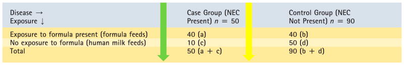
        3. OR is often used in case-control studies. Table 5 depicts a case-control study. Fifty patients with NEC are matched with 90 patients without NEC. The odds of being exposed (to formula feeds) among subjects (preterm infants) with and without an event (NEC) is calculated. The OR of exposure to formula feeds among preterm infants with NEC is a/c ÷b/d = 40/10 ÷40/50 = 5.

        4. OR approximates relative risk if the event rates in the whole population are uncommon.

        5. As the magnitude of risk (event rates) in the unexposed population increases, then OR will NOT approximate relative risk.

     3. Similar to relative risk, an OR of 1 indicates no association between exposure and outcome. An OR more than 1 indicates positive association and less than 1 indicates negative association.

     4. Confidence intervals (typically at 95%) for relative risk and OR indicate that the investigator can be 95% confident that the real relative risk or OR in the population lies within this range of values. If the 95% confidence interval crosses 1, the association is not significant. If both the confidence limits exceed 1 (for example, 2.7 to 7.2), there is a significant positive association between exposure and outcome. If both the confidence limits are less than 1, there is a significant negative association between exposure and outcome (for example, 0.6 to 0.92). If the confidence limits cross 1 (for example, 0.98 to 1.75), there is no significance.

• (5)Correlation coefficient (r) quantifies the degree to which two random variables are related, provided that the relationship is linear.

  1. Correlation coefficient can range from −1 to +1. A positive value, 0.78 for example, indicates a positive relationship and a negative value indicates a negative relationship (if one variable increases, the other decreases).

  2. The regression line is the straight line passing through the data that minimizes the sum of the squared differences between the original data and the fitted points.

  3. The strength of correlation is dependent on the slope of the regression line. If the value is close to 1 (or −1), the regression line has a steep slope and the correlation is high; if correlation coefficient is 0, the two variables are independent of each other.

  4. Properties of correlation

     1. Assumes that each variable is normally distributed (works if one of the variables is binary)

     2. Measures linear relationship only

     3. Affected by variances of the variable in addition to association

     4. Extreme values or pairs are highly influential

  5. Limitations of correlation coefficient

     1. Cannot assess for nonlinear relationships

     2. Increasing sample size leads to “significance” at lower r values. For example, If n = 40, r > 0.7 may provide significance; but if n > 400, r = 0.15, may provide significance.

     3. The estimated correlation should only not be extrapolated beyond the observed range of the variables, the relationship may be different outside this region.

     4. Correlation does not equal causation.

Table 5.

Case-Control Study

Fifty patients with necrotizing enterocolitis (NEC) are matched with 90 control subjects who do not have NEC. Both groups are evaluated with respect to exposure to formula feeds.

Hazard ratio

1. Hazard ratio is a measure of relative risk over time in circumstances in which we are interested not only in the total number of events, but in their timing as well. The timing may be represented as child months or line days and so forth.

2. The event of interest may be death or it may be a nonfatal event, such as readmission, line infection, or symptom change.

6. Regression Analysis

Regression analysis is a method used to explore the nature of relationship between two continuous random variables. Regression allows us to estimate the degree of change in one variable (response variable) to a unit change in the second variable (explanatory variable).

1. Simple regression: Many relationships between variables can be fit to a straight line. For example, the change in head circumference with change in gestational age can be represented by the equation for a straight line.

   $$\mathrm{y}={\mathrm{\beta }}_0+{\mathrm{\beta }}_1\mathrm{x}+\mathrm{\epsilon },$$

   where “y” is the mean head circumference at gestational age of “x” weeks;

   β₀ is the y-intercept (mean value of the response y when x = 0, although this is not clinically applicable for the current example);

   β₁ is the slope of the line (change in mean value of y that corresponds to a 1 unit increase in x); and

   ε is the distance of a given observation from the population regression line (because y is the mean head circumference, each infant’s head circumference will be scattered around the mean and not necessary exactly equal to the mean).

   This is the simple linear regression equation and can be used when the relationship between the two variables is roughly linear. Multiple regression involves the linear relationship between one dependent variable, for example, presence or absence of bronchopulmonary dysplasia and multiple explanatory variables (eg, duration of mechanical ventilation, duration of oxygen exposure, infection, nutrition, gestational age). The equation for multiple regression is

   $$\mathrm{Y}={\mathrm{\beta }}_0+{\mathrm{\beta }}_1{\mathrm{x}}_1+{\mathrm{\beta }}_2{\mathrm{x}}_2+\dots +{\mathrm{\beta }}_{\mathrm{i}}{\mathrm{x}}_{\mathrm{i}}+\mathrm{\epsilon }$$

2. Logistic regression: In situations in which the response of interest is dichotomous (binary) rather than continuous, linear regression cannot be used to explore the nature of the relationship. For example if the outcome is mortality, the two outcomes possible are alive or dead. In such a situation, the probability of being alive or dead is the response that is estimated for various values of the explanatory variable using a technique known as logistic regression.

   1. The variables cannot be plotted on a straight line but may have a sigmoid configuration and need logistic transformation (change to an equation to the power of “e,” where “e” is the base of natural logarithm).

   2. The logistic function is given by the equation:

      $$\mathrm{p}=\frac{e^{\beta 0+\beta 1x}}{1+e^{\beta 0+\beta 1x}}$$

      The interpretation of β0 and β1 are in the log odds scale.

3. Survival analysis: A model to analyze time to event.

   1. The response value of interest is the amount of time from an initial observation to the occurrence of an event. In addition to studies evaluating change in mortality, survival analysis can be used in studies in which time to an event is an outcome; for example, time to relapse after chemotherapy for a malignancy.

   2. In survival analysis, not all individuals are observed until their “event.” The data may be analyzed before the event has occurred in all patients. Some patients may be “lost to follow-up” for a variety of reasons and their data may not be available for some duration of the study. The incomplete observation of the time to event is known as censoring and is shown as a notch (Fig 8).

   3. A common method used is the product limit method (also called the Kaplan-Meier method). This is a nonparametric technique (no assumption about the distribution of population, not smooth) that uses the exact survival time for each subject in a sample (instead of grouping the times into intervals, Fig 8).

   4. Proportional hazards assumption (Cox): In the Cox proportional hazards assumption, curves will not cross; risk of relapse in one group is a fixed proportion of the risk in the other group. Curves are less reliable as the number of subjects decreases (so may cross toward the end even if the proportional hazards assumption is mostly true). The proportional hazards model can assess the effects of multiple covariates on survival.

Figure 8.

Interpretation of a Kaplan-Meier curve (based on Mah D, Singh TP, Thiagarajan RR, et al. Incidence and risk factors for mortality in infants awaiting heart transplantation in the USA. J Heart Lung Transplant. 2009;28(12):1292–1298; ticks/ notches are added to the original curve for educational purposes) ECMO=extracorporeal membrane oxygenation.

7. Diagnostic Tests

1. GOLD STANDARD diagnostic test is an unambiguous method of determining whether or not a patient has a particular disease or outcome. For example, a positive bacterial culture in blood or cerebrospinal fluid with an organism that is not considered a contaminant in that age group is the gold standard for bacteremia/sepsis. A test being evaluated for early detection of neonatal sepsis (such as elevated C-reactive protein [CRP]) is often tested against the gold standard (positive blood culture). A gold standard test has the following limitations:

   1. Incorporation bias: If any symptoms, signs, or laboratory tests used to diagnose a disease are used as part of the gold standard (such as the Centers for Disease Control and Prevention’s definition of ventilator-associated pneumonia in infants that includes chest X-ray, hypoxia, temperature instability, abnormal white count, and so forth), a study comparing one of these components (such as leukopenia) to that gold standard can make them look falsely good. Hence, it is important to have an independent gold standard while evaluating a diagnostic test.

   2. If the gold standard is imperfect, it can make a test look either worse or better than it really is.

   3. If the test has continuous results (like CRP), a cutoff point (such as CRP >10 mg/L) is necessary to define a positive test.

2. SENSITIVITY AND SPECIFICITY: When results of a new diagnostic test with dichotomous results are compared with a dichotomous gold standard, the results can be summarized in a 2 × 2 table (Table 6).

   1. Sensitivity of a test is defined as the proportion of subjects with the disease in whom the test gives the correct answer (true-positive, Fig 9A and Table 6).

      1. A highly sensitive test has a low false-negative rate and is good as a screening test and a negative test almost rules out the disease.

      2. It is calculated as true-positives ÷ (true-positives + false-negatives, ie, all subjects with the disease).

   2. Specificity is the proportion of subjects without the disease in whom the test gives the right answer (true-negative).

      1. A highly specific test has a low false-positive rate.

      2. It is calculated as true-negatives ÷ (false-positives + true-negatives, ie, all subjects without the disease).

3. PREDICTIVE VALUES:

   1. Positive predictive value (PPV) is the proportion of subjects with positive tests who have the disease. It is calculated by true-positives ÷ (true-positives + false-positives, ie, all subjects who tested positive with the test).

   2. Negative predictive value (NPV) is the proportion of subjects with negative tests who do not have the disease. It is calculated by true-negatives ÷ (false-negative + true-negative).

4. Effect of disease prevalence:

   1. Sensitivity and specificity are prevalence-independent test characteristics, as their values are intrinsic to the test and do not depend on the disease prevalence in the population of interest.

   2. Increased prevalence of disease will increase PPV and decrease NPV (Fig 9B and Table 7).

   3. Reduced disease prevalence will decrease PPV and increase NPV.

5. Receiver operator characteristic (ROC) curve (Fig 10): Many diagnostic tests yield ordinal or continuous (interval or ratio) results. For example, if serum CRP is measured at 6 hours after birth to diagnose early-onset sepsis, a cutoff value of 1 mg/L to define a positive test may yield different sensitivity and specificity compared with a cutoff value of 10 mg/L. Similarly, different white blood cell count ranges provide different sensitivities and specificities for predicting serious bacterial infection in newborn infants. (6) Typically, increasing the threshold for a positive test reduces false-positives and increases specificity. In contrast, reducing the threshold or cutoff value for a positive test reduces false-negatives and increases sensitivity. This tradeoff between sensitivity (ie, true-positive rate on y-axis) and specificity (as 1 – specificity or false-positive rate on the x-axis) is graphically depicted in the ROC curve (Fig 10).

   1. The area under the ROC curve is a useful summary of the overall accuracy of a test.

   2. The area under the ROC curve ranges from 0.5 (a diagonal from lower-left to upper-right corner and a useless test) to 1.0 (a curve along the left and upper borders for a perfect test).

6. Likelihood ratio: For each test result, the likelihood ratio is the ratio of the likelihood of that result in someone with the disease to the likelihood of that result in someone without the disease.

   1. For dichotomous tests, the likelihood ratio for a positive test is sensitivity/(1-specificity) and the likelihood ratio of a negative test is (1−sensitivity/ specificity).

   2. For example, if 19% of neonates with serious bacterial infection and 0.52% of neonates without a serious bacterial infection have a white count less than 5,000/μL, the likelihood ratio for serious bacterial infection in a neonate with leukopenia is 19/0.52 = 36. (7)

   3. The probability of the disease is known from clinical history and status and existing literature before the test is the pretest odds or prior odds. For example, assume that the pre–complete blood count test odds for an African American infant born at 35 weeks by vaginal delivery to have early-onset sepsis is 1/1,000 live births. If a complete blood count is performed at 6 hours after birth and the white blood cell count is less than 5,000/μL, the posttest odds or posterior odds of this infant having a serious bacterial infection is 36/1,000 live births.

   4. Posterior odds (posttest odds) = Prior odds × Likelihood ratio

7. Clinical prediction rule is an algorithm that combines several predictors, including the presence or absence of various symptoms, signs, and laboratory tests, to estimate the probability of a particular disease or outcome.

   1. The goal is to improve clinical decisions using mathematical methods involving multivariate techniques. Points can be assigned to various risk factors, signs, and symptoms to derive a predictive score.

   2. An alternative approach is to create a decision tree by using a series of yes/no questions and is called recursive partitioning or classification and regression tree analysis. These techniques are being used to predict the risk of sepsis in neonates more than 34 weeks’ gestation (8)(9) and optimize use of antibiotics for suspected early-onset sepsis in neonates.

   3. Clinical prediction rules should be validated to avoid overfitting (random error to increase the predictive score from a single sample).

      1. Internal validity (within the study sample) can be tested by dividing the cohort used to derive the clinical prediction rule into derivation (one-half to two-thirds of the sample) and validation data sets. The rule derived from the derivation cohort is then tested in the validation cohort. (8)

      2. External validity is assessed by prospective validation by testing the rule in different populations.

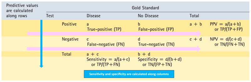
Table 6.

Calculation of Sensitivity, Specificity, PPV, and NPV

Note:

1. Disease is the first row (on the top) and test is the first column by convention.
2. The numerator for predictive values and sensitivity/ specificity is always a TRUE value (TN or TP).
3. Sensitivity/specificity are calculated along columns and rows are associated with predictive value calculations (see above).
4. A highly sensitive test is used to rule out disease (SnOUT): low false-negative rate.
5. A highly specific test is used to rule in disease (SpIN): low false-positive rate.

NPV=negative predictive value, PPV=positive predictive value.

Figure 9.

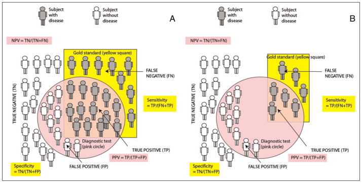
A. Sensitivity, specificity, and positive predictive value (PPV) and negative predictive value (NPV), the gold standard for diagnosis, identifies patients with disease (shown as gray subjects) located in the yellow square. Subjects without disease are shown in white color. The diagnostic test is positive in subjects located inside the pink circle. B. The impact of reduced disease prevalence on PPV and NPV. The number of subjects with the disease (based on the gold standard test) decreases secondary to reduced prevalence. Because of a reduction in the number of true positive (TP) subjects, PPV decreases. NPV increases because of a decrease in false-negative (FN) subjects. Sensitivity and specificity are not influenced by disease prevalence. The effect of increased prevalence is opposite of the change in predictive values associated with reduced disease prevalence and is shown in Table 7 (increased PPV and decreased NPV).

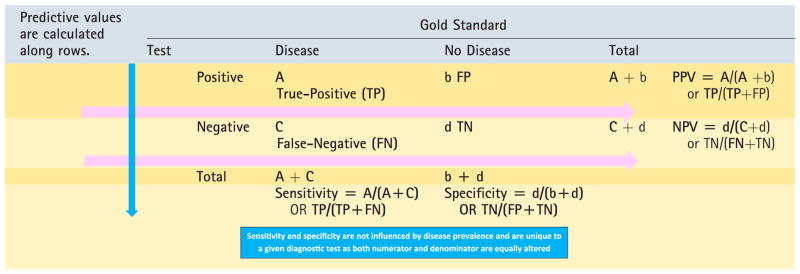
Table 7.

Effect of Increased Prevalence of Disease on Sensitivity, Specificity, and Predictive Values

Upper case letters in bold indicate increased number due to increased disease prevalence. NPV, negative predictive value, PPV=positive predictive value.

Figure 10.

Receiver operator characteristic (ROC) curves for a good test (shown with green dashed line) and a poor/ worthless test (shown with red dashed line). The area under the curve provides a measure of the capability of the test. The area under curve for the good test is shown with green dots and is close to 1.0. The area under the curve for the poor test is close to 0.5 (50% chance of diagnosing the disease) and is shown by a red shade.

Conclusions

A basic understanding of biostatistics is necessary for a neonatal practitioner. This is useful in interpretation of studies and journal articles. Clinicians conducting research require a thorough knowledge of biostatistics. This review is intended to provide a quick overview of biostatistics for trainees or as a refresher for neonatologists during preparation for a pediatric subspecialty board certification.

American Board of Pediatrics Neonatal-Perinatal Content Specifications.

• Distinguish types of variables (eg, continuous, categorical, ordinal, nominal).

• Understand how the type of variable (eg, continuous, categorical, nominal) affects the choice of statistical test).

• Understand how distribution of data affects the choice of statistical test.

• Differentiate normal from skewed distribution of data.

• Understand the appropriate use of the mean, median, and mode.

• Understand the appropriate use of standard deviation (SD).

• Understand the appropriate use of standard error (SE).

• Distinguish the null hypothesis from an alternative hypothesis.

• Interpret the results of hypothesis testing.

• Understand the appropriate use of the χ² test versus a t test.

• Understand the appropriate use of analysis of variance (ANOVA).

• Understand the appropriate use of parametric (eg, t test, ANOVA) versus nonparametric (eg, Mann-Whitney U, Wilcoxon) statistical tests.

• Interpret the results of χ² tests.

• Interpret the results of t tests.

• Understand the appropriate use of a paired and nonpaired t test.

• Determine the appropriate use of a one-versus two-tailed test of significance.

• Interpret a P value (probability of the null hypothesis being true by chance alone).

• Interpret a P value when multiple comparisons have been made.

• Interpret a confidence interval.

• Identify a type I error.

• Identify a type II error.

• Differentiate relative risk reduction from absolute risk reduction.

• Calculate and interpret a relative risk.

• Calculate and interpret an odd ratio (OR).

• Understand the uses and limitations of a correlation coefficient.

• Identify when to apply regression analysis (eg, linear, logistic).

• Interpret a regression analysis (eg, linear, logistic).

• Identify when to apply survival analysis (eg, Kaplan-Meier).

• Interpret a survival analysis (eg, Kaplan-Meier).

• Recognize the importance of an independent “gold standard” in evaluating a diagnostic test.

• Calculate and interpret sensitivity and specificity.

• Calculate and interpret positive predictive values (PPVs) and negative predictive values (NPVs).

• Understand how disease prevalence affects the PPV and NPV of a test.

• Calculate and interpret likelihood ratios.

• Interpret a receiver operator characteristic (ROC) curve.

• Interpret and apply a clinical prediction rule.

Abbreviations

ANOVA

analysis of variance

CRP

C-reactive protein

ECMO

extracorporeal membrane oxygenation

IQR

interquartile range

NEC

necrotizing enterocolitis

NPV

negative predictive value

OR

odds ratio

PDA

patent ductus arteriosus

PPV

positive predictive value

ROC

receiver operator characteristic