New Statistical Learning Methods for Estimating Optimal Dynamic Treatment Regimes

Abstract

Dynamic treatment regimes (DTRs) are sequential decision rules for individual patients that can adapt over time to an evolving illness. The goal is to accommodate heterogeneity among patients and find the DTR which will produce the best long term outcome if implemented. We introduce two new statistical learning methods for estimating the optimal DTR, termed backward outcome weighted learning (BOWL), and simultaneous outcome weighted learning (SOWL). These approaches convert individualized treatment selection into an either sequential or simultaneous classification problem, and can thus be applied by modifying existing machine learning techniques. The proposed methods are based on directly maximizing over all DTRs a nonparametric estimator of the expected long-term outcome; this is fundamentally different than regression-based methods, for example Q-learning, which indirectly attempt such maximization and rely heavily on the correctness of postulated regression models. We prove that the resulting rules are consistent, and provide finite sample bounds for the errors using the estimated rules. Simulation results suggest the proposed methods produce superior DTRs compared with Q-learning especially in small samples. We illustrate the methods using data from a clinical trial for smoking cessation.

1 Introduction

It is widely-recognized that the best clinical regimes are adaptive to patients over time, observing that there exists significant heterogeneity among patients, and moreover, that often the disease is evolving and as diversified as the patients themselves (Wagner et al., 2001). Treatment individualization and adaptation over time is especially important in the management of chronic diseases and conditions. For example, treatment for major depressive disorder is usually driven by factors emerging over time, such as side-effect severity, treatment adherence and so on (Murphy et al., 2007); the treatment regimen for non-small cell lung cancer involves multiple lines of treatment (Socinski and Stinchcombe, 2007); and clinicians routinely update therapy according to the risk of toxicity and antibiotics resistance in treating cystic fibrosis (Flume et al., 2007). As these examples make clear, in many cases a “once and for all” treatment strategy is not only suboptimal due to its inflexibility but unrealistic (or even unethical). In practice, treatment decisions must adapt with time-dependent outcomes, including patient response to previous treatments and side effects. Moreover, instead of focusing on short-term benefit of a treatment, an effective treatment strategy should aim for long-term benefits by accounting for delayed treatment effects.

Dynamic treatment regimes (DTRs), also called adaptive treatment strategies (Murphy, 2003, 2005a), are sequential decision rules that adapt over time to the changing status of each patient. At each decision point, the covariate and treatment histories of a patient are used as input for the decision rule, which outputs an individualized treatment recommendation. In this way, both heterogeneity across patients and heterogeneity over time within each patient are taken into consideration. Thus, various aspects of treatment regimes, including treatment types, dosage levels, timing of delivery, etc., can evolve over time according to subject-specific needs. Treatments resulting in the best immediate effect may not necessarily lead to the most favorable long-term outcomes. Consequently, with the flexibility of managing the long-term clinical outcomes, DTRs have become increasingly popular in clinical practice. In general, the goal is to identify an optimal DTR, defined as the rule that will maximize expected long-term benefit.

A convenient way to formalize the problem in finding optimal DTRs is through potential outcomes (Rubin, 1974, 1978; Robins, 1986; Splawa-Neyman et al., 1990), the value of the response variable that would be achieved, if perhaps contrary to fact, the patient had been assigned to different treatments. Potential outcomes can be compared to find the regime that leads to the highest expected outcome if followed by the population. However, potential outcomes are not directly observable, since we can never observe all the results that could occur under different treatment regimes on the same patient. A practical design that facilitates the connection of potential outcomes with observed data is the sequential multiple assignment randomized trial (SMART) (Lavori and Dawson, 2000, 2004; Dawson and Lavori, 2004; Murphy, 2005a; Murphy et al., 2007). In this design, patients are randomized at every decision point. SMART designs guarantee that treatment assignments are independent of potential future outcomes, conditional on the history up to the current time, resulting in the validity of the so-called ‘no unmeasured confounders’ or ‘sequential ignorability’ assumption. The latter condition guarantees that the optimal DTRs can be inferred from observed data in the study (Murphy et al., 2001).

A number of methods have been proposed to estimate the optimal DTRs. Lavori and Dawson (2000) used multiple imputation to estimate all potential outcomes, so that the adaptive regimes can be compared using the imputed outcomes. Murphy et al. (2001) employed a structural model to estimate the mean response that would have been observed if the whole population followed a particular DTR. Likelihood-based approaches were proposed by Thall et al. (2000, 2002, 2007), where both frequentist and Bayesian methods are applied to estimate parameters and thus the optimal regimes. All these approaches first estimate the data generation process via a series of parametric or semiparametric conditional models, then estimate the optimal DTRs based on the inferred data distributions. These approaches easily suffer from model misspecification due to the inherent difficulty of modeling accumulative time-dependent and high-dimensional information in the models.

Machine learning methods are an alternative approach to estimating DTRs that have gained popularity due in part to their avoidance of having to completely model the underlying generative distribution. Two common learning approaches are Q-learning (Watkins, 1989; Sutton and Barto, 1998) and A-learning (Murphy, 2003; Blatt et al., 2004), where ‘Q’ denotes ‘quality’ and ‘A’ denotes ‘advantage’. The Q-learning algorithm, originally proposed in the computer science literature, has become a powerful tool to discover optimal DTRs in the clinical research arena (Murphy et al., 2007; Pineau et al., 2007; Zhao et al., 2009; Nahum-Shani et al., 2012). Q-learning is an approximate dynamic programming procedure that estimates the optimal DTR by first estimating the conditional expectation of the sum of current and future rewards given the current patient history and assuming that optimal decisions are made at all future decision points. The foregoing conditional expectations are known as Q-functions. In Q-learning and related methods, the Q-function can be modeled parametrically, semiparametrically and even nonparametrically (Zhao et al., 2009). In A-learning, proposed by Murphy (2003), one models regret functions which measure the loss incurred by not following the optimal treatment regime at each stage. Minimizing the regret functions leads to the optimal decision rule at each stage. It has been shown that A-learning is a special case of a structural nested mean model (Robins, 2004; Moodie et al., 2007). For more discussion on the relationship between Q- and A-learning see Schulte et al. (2014). One limitation of Q- and A-learning is that the optimal DTRs are estimated in a two-step procedure: one estimates either the Q-functions or the regret functions using the data; then these functions are either maximized or minimized to infer the optimal DTRs. In the presence of high-dimensional information, it is possible that either the Q-functions or the regret functions are poorly fitted, and thus the derived DTR may be far from optimal. Moreover, estimation based on minimizing the prediction errors in fitting the Q-functions or the regret functions may not necessarily result in maximal long-term clinical benefit. This was demonstrated by Zhao et al. (2012) in the case of a single treatment decision who subsequently proposed an alternative method that maximizes an estimator of the expected clinical benefit. Zhao et al. (2012) proposed an alternative to regression in the setting where there is no need to consider future treatments or outcomes. Generalizing this approach to the multi-stage setting is non-trivial since one must account for long-term cumulative outcomes. Other approaches to direct maximization include robust estimation (Zhang et al., 2013) and the use of marginal structural mean models (Orellana et al., 2010). Zhang et al. (2013) used a stochastic search algorithm to directly optimize an estimator for the mean outcome over all DTRs within a restricted class for a sequence of treatment decisions. However, this approach involves maximizing a discontinuous objective function and becomes extremely computationally burdensome in problems with a moderate number of covariates. Furthermore, theoretical results for this approach are currently unknown.

In this paper, we propose two original approaches to estimating an optimal DTR. Whereas Zhao et al. (2012) proposed an alternative to regression we propose an alternative approach to regression-based approximate dynamic programming algorithms. This requires nontrivial methodological and algorithmic developments. We first develop a new dynamic statistical learning procedure, backward outcome weighted learning (BOWL), which recasts estimation of an optimal DTR as a sequence of weighted classification problems. This approach can be implemented by modifying existing classification algorithms. We also develop a simultaneous outcome weighted learning (SOWL) procedure, which recasts estimation of an optimal DTR as a single classification problem. To our knowledge, this is the first time that learning multistage decision rules (optimal DTRs) is performed simultaneously and integrated into a single algorithm. Current algorithms from SVMs are adjusted and further developed for SOWL. We demonstrate that both BOWL and SOWL consistently estimate the optimal decision rule and they provide better DTRs than Q- and A-learning in simulated experiments. The contributions of our work include:

1. A new paradigm for framing the problem of estimating optimal DTRs by aligning it with a weighted classification problem where weights depend on outcomes.

2. Two fundamentally new statistical learning methodologies, BOWL and SOWL, which are entirely motivated by the problem of DTR estimation.

3. Easy-to-use computing algorithms and software. Users familiar with existing learning algorithms (especially SVMs) can readily understand and modify our methods.

4. A new perspective on estimating optimal DTRs. This perspective motivates future work on multi-arm trials, optimal dose finding, censored data, high-dimensional feature selection in DTRs, etc. We are confident that other researchers will be able to contribute a great deal to this rapidly growing area.

The remainder of the paper is organized as follows. In Section 2, we formalize the problem of estimating an optimal DTR in a mathematical framework. We then reformulate this problem as a weighted classification problem and based on this reformulation we propose two new learning methods for estimating the optimal DTR. Section 3 provides theoretical justifications for the proposed methods including consistency and risk bound results. We present empirical comparisons of the proposed methods with Q- and A-learning in Section 4. Section 5 focuses on the application of the proposed methods for the multi-decision setup, where the data comes from a smoking cessation trial. Finally, we provide a discussion of open questions in Section 6. The proofs for the theoretical results are given in the Appendix.

2 General Methodology

2.1 Dynamic Treatment Regimes (DTRs)

Consider a multistage decision problem where decisions are made in T stages. For j = 1, …, T, let A_j be a dichotomous treatment with values in = {−1, 1}, which is the treatment assigned at the j^th stage, X_j be the observation after treatment assignment A_j−1 but prior to j^th stage, and X_T+1 denotes the covariates measured at the end of stage T. Note that more generally A_j might be multi-category or continuous; however, we do not consider these cases here (see Section 6). Following j^th treatment, there is an observed outcome, historically termed the “reward.” We denote the j^th reward by R_j and assume it is bounded and has been coded so that larger values correspond to better outcomes. In most settings, R_j depends on all precedent information, which consists of all the covariate information, X₁, …, X_j, treatment history, A₁, …, A_j, and historical outcomes, R₁, …, R_j−1. Note that R_j can be a part of X_j+1. The overall outcome of interest is the total reward ${\sum }_{j=1}^T{R}_j$.

A DTR is a sequence of deterministic decision rules, d = (d₁, …, d_T), where d_j is a map from the space of history information H_j = (X₁, A₁, …, A_j−1, X_j), denoted by , to the space of available treatments . The value associated with a regime d (Qian and Murphy, 2011) is

$$V^{\mathbf{d}}=E_{\mathbf{d}}\left[\sum _{j=1}^T{R}_j\right]=\int \sum _{j=1}^T{R}_j{dP}_{\mathbf{d}},$$

where P_d is the measure generated by the random variables (X₁, A₁, X₂, R₁, …, A_T, X_T+1, R_T) under the given regime, i.e., A_j = d_j(H_j) and E_d denotes expectation against P_d. Thus, V^d is the expected long-term benefit if the population were to follow the regime d. Let P denote the measure generated by (X₁, A₁, …, A_T, X_T+1, R_T) from which the observed data are drawn, and let E denote expectation taken with respect to this measure. Under the following conditions, which are assumed hereafter, V^d can be expressed in terms of P:

1. A_j is randomly assigned with probability possibly dependent on H_j, j = 1, …, T (sequential multiple assignment randomization);

2. with probability one, π_j(a_j, H_j) = P(A_j = a_j|H_j) ∈ (c₀, c₁) for any a_j ∈ , where 0< c₀ < c₁ < 1 are two constants, and π_j is assumed to be known.

The foregoing assumptions are satisfied when data are collected in a SMART (Lavori and Dawson, 2004). Under these assumptions it can be shown that P_d is dominated by P and

$$\frac{{dP}_{\mathbf{d}}}{dP}=\frac{{\prod }_{j=1}^{T}I(A_j=d_j(H_j))}{{\prod }_{j=1}^T{\pi }_j(A_j,H_j)},$$

where I(·) is the indicator function. As a result,

$$V^{\mathbf{d}}=\int \sum _{j=1}^T{R}_j\frac{{dP}_{\mathbf{d}}}{dP}dP=E\left[\frac{\left({\sum }_{j=1}^T{R}_j\right){\prod }_{j=1}^{T}I(A_j=d_j(H_j))}{{\prod }_{j=1}^T{\pi }_j(A_j,H_j)}\right].$$ (2.1)

When T = 1, the value function of assigning treatment A₁ = 1 to all patients is simply a weighted average of all outcomes among those that received A₁ = 1 with weights π₁(A₁, H₁)⁻¹. The optimal value function is defined as V^* = , where consists of all possible regimes, and the optimal DTR, denoted by d^*, is the regime yielding V^*. The goal is to estimate d^* from data. Note that d^* remains unchanged if R_j is replaced by R_j + c for any constant c. Hence, we assume R_j ≥ 0, j = 1, …, T.

When the underlying generative distribution is known, dynamic programming shows that $d_T^{\ast }(h_T)=arg{max}_{a_T}{Q}_T(h_T,a_T)$ where Q_T (h_T, a_T) = E(R_T|H_T = h_T, A_T = a_T) and recursively $d_j^{\ast }(h_j)=arg{max}_{a_j}{Q}_j(h_j,a_j)$ where Q_j (h_j, a_j) = E(R_j + max_aj+1 Q_j+1(H_j+1, a_j+1)|H_j = h_j, A_j = a_j) for j = T − 1, …, 1 (Bellman, 1957; Sutton and Barto, 1998). Q-learning is an approximate dynamic programming algorithm that uses regression models to estimate the Q-functions Q_j(h_j, a_j) j = 1, …, T. Linear working models are typically used to approximate the Q-functions. However, Murphy (2005b) show that there is a mismatch between the estimand in Q-learning and the optimal DTR. This mismatch results from the fact that Q-learning targets the optimal Q-function rather than directly targeting the optimal regime. A postulated class of Q-functions induces a corresponding class of DTRs, namely those representable as the arg max of the postulated Q-functions. Qian & Murphy (2011) show that Q-learning can be inconsistent when the postulated Q-functions are misspecified even in cases where the optimal DTR resides in the class of induced DTRs.

2.2 A Different View of Estimating the Optimal DTR

Our proposed methodology takes a completely different approach to estimating the optimal DTR. Generally speaking, existing methods model the temporal relationship between the historical information and future rewards, e.g., modeling the Q-functions in Q-learning or modeling the regret functions in A-learning, and then invert this relationship to estimate the optimal DTR. In contrast, our proposed approaches examine the data retrospectively by investigating the differences between subjects with observed high and low rewards, so as to determine what the optimal treatment assignments should be relative to the actual treatments received for different groups of patients. From this perspective, the optimal DTR estimation can be reformulated as a weighted classification problem. We can thus incorporate statistical learning techniques into the DTR estimation framework.

To provide intuition we first consider the single stage estimation (T = 1) problem considered by Zhao et al. (2012). Since T = 1, we omit the subscript so the observed random variables only include baseline covariates X, treatment assignment A, and observed reward R. Then the value function associate with a treatment regime d is E_d(R) = E[RI(A = d(X))/π(A, X)]. Identifying the treatment rule d^* which maximizes E_d(R) is equivalent to finding the d^* which minimizes E[RI(A ≠ d(X))/π(A, X)]. This objective can be viewed as a weighted misclassification error, with the weight for each misclassification event given by R/π(A, X). Intuitively, minimizing this objective implies that subjects with high observed rewards are more likely to be assigned to the treatment actually received whereas subjects with low observed rewards are more likely to be assigned to the treatment not actually received. Hence, we view maximizing the value function as minimizing a retrospective outcome weighted 0–1 loss function.

Direct minimization of the empirical analogue of the V^d is difficult due to the non-convex and discontinuous 0–1 loss. Inspired by the fact that without the weights the objective would be the same as commonly used in classification, Zhao et al. (2012) proposed to use a convex surrogate loss for the 0–1 loss, which has been widely applied in the classification literature (Hastie et al., 2009). Support vector machines (SVMs, Cortes and Vapnik, 1995), enjoy optimality properties and fast algorithms which Zhao et al. (2012) showed can be translated to the treatment selection problem. In particular, they replaced the 0–1 loss with a hinge loss in the empirical analogue of the objective, and subsequently estimated the optimal decision function by minimizing

$$n^{-1}\sum _{i=1}^n\frac{R_i}{\pi (A_i,X_i)}\varphi (A_{i}f(X_i))+{\lambda }_n{\Vert f\Vert }^2$$ (2.2)

based on the data from n subjects, where: f(x) is the decision function so that d(x) = sign(f(x)); ϕ(v) = max(1 − v, 0) is the hinge loss; and λ_n is the tuning parameter controlling the severity of the penalty and ||f||. Typically, ||f|| is the Euclidean norm of β if f(x) = 〈 β, x 〉 + β₀, where 〈 a, b 〉 = a^Tb is the inner product in Euclidean space, or ||f|| is given by the norm in a reproducing kernel Hilbert space (RKHS). Zhao et al. (2012) established theoretical properties and demonstrated superior empirical performance over a regression-based approach.

However, the method in Zhao et al. (2012) cannot be directly generalized to estimating optimal DTRs, due to the fact that optimal DTRs need to be determined for multiple stages and the estimation at stage t depends on the decision for the treatment regimes at future stages. To deal with this problem, we propose two distinct new nonparametric learning approaches in the following sections: one sequentially estimates optimal DTRs by means of outcome weighted learning, and the other simultaneously learns optimal DTRs across all stages.

2.3 Approach 1: Backward Outcome Weighted Learning (BOWL)

DTRs aim to maximize the expected cumulative rewards, hence, the optimal treatment decision at the current stage must depend on subsequent decision rules. This motivates a backwards recursive procedure which estimates the optimal decision rule at future stages first, and then the optimal decision rule at current stage by restricting the analysis to the subjects who have followed the estimated optimal decision rules thereafter. Assume that we observe data (X_i1, A_i1, …, A_iT, X_i,T+1, R_iT), i = 1, …, n forming n independent and identically distributed patient trajectories from a SMART. Suppose that we already possess the optimal regimes at stages t + 1, …, T and denote them as $d_{t+1}^{\ast },\dots ,d_T^{\ast }$. Then the optimal decision rule at stage t, $d_t^{\ast }(h_t)$ should maximize

$$E\left[\frac{({\sum }_{j=t}^T{R}_j){\prod }_{j=t+1}^{T}I(A_j=d_j^{\ast }(H_j))}{{\prod }_{j=t}^T{\pi }_j(A_j,H_j)}I(A_t=d_t(H_t))|H_t=h_t\right],$$

where we assume all subjects have followed the optimal DTRs after stage t. Hence, $d_t^{\ast }$ is a map from to {−1, 1} which minimizes

$$E\left[\frac{({\sum }_{j=t}^T{R}_j){\prod }_{j=t+1}^{T}I(A_j=d_j^{\ast }(H_j))}{{\prod }_{j=t}^T{\pi }_j(A_j,H_j)}I(A_t\ne d_t(H_t))\right],$$ (2.3)

This suggests that we minimize the empirical analog of the above expression using the data from the n subjects, given that we know the optimal decisions in the future. This is equivalent to an empirical average of a weighted 0–1 loss functions, where the weights are defined by $({\sum }_{j=t}^T{R}_{ij}){\prod }_{j=t+1}^{T}I(A_{ij}=d_j^{\ast }(H_{ij}))/{\prod }_{j=t}^T{\pi }_j(A_{ij},H_{ij})$ for each individual. We develop a tractable estimation procedure by using a convex surrogate for the 0–1 loss for stage t. We use hinge loss throughout this paper, although any other sensible loss function could also be used.

Let f_t : ↦ ℝ denote the decision function at stage t, so that d_t(h_t) = sign(f_t(h_t)), were $d_{t+1}^{\ast },\dots ,d_T^{\ast }$ known we could minimize with respect to f_t:

$$n^{-1}\sum _{i=1}^n\frac{({\sum }_{j=t}^T{R}_{ij}){\prod }_{j=t+1}^{T}I(A_{ij}=d_j^{\ast }(H_{ij}))}{{\prod }_{j=t}^T{\pi }_j(A_{ij},H_{ij})}\varphi (A_{it}{f}_t(H_{it}))+{\lambda }_{t,n}{\Vert f_t\Vert }^2.$$

The objective function at stage t has a similar form as (2.2), except that the weight incorporates future information. The estimator uses data from the subjects whose actual treatment assignments are the same as the future optimal treatments in stages t + 1, …, T to learn the optimal rule at stage t.

Since future optimal decisions are unknown, we first estimate the optimal decision rule at the last stage and then proceed backwards recursively. At each stage, we conduct the optimization based on the subjects who have followed the constructed optimal DTRs in the later stages. The BOWL estimation algorithm is as follows.

Step 1

Minimize

$$n^{-1}\sum _{i=1}^n\frac{R_{iT}\varphi (A_{iT}{f}_T(H_{iT}))}{{\pi }_T(A_{iT},H_{iT})}+{\lambda }_{T,n}{\Vert f_T\Vert }^2$$ (2.4)

with respect to f_T and let f̂_T denote the minimizer. Then the estimated optimal decision rule is d̂_T(h_T) = sign(f̂_T(h_T)). This minimization is equivalent to the single-stage outcome weighted learning in Zhao et al. (2012) and it has a similar dual objective function to the usual SVM, which can be implemented via quadratic programming.

Step 2

For t = T − 1, T − 2, …, 1, we backwards sequentially minimize

$$n^{-1}\sum _{i=1}^n\frac{({\sum }_{j=t}^T{R}_{ij}){\prod }_{j=t+1}^{T}I(A_{ij}={\widehat{d}}_j(H_{ij}))}{{\prod }_{j=t}^T{\pi }_j(A_{ij},H_{ij})}\varphi (A_{it}{f}_t(H_{it}))+{\lambda }_{t,n}{\Vert f_t\Vert }^2,$$ (2.5)

where the d̂_t+1, …, d̂_T are obtained prior to stage t. Note that each minimization can still be carried out using the same algorithm in Step 1 except that the individual weights in front of the hinge loss are replaced by $({\sum }_{j=t}^T{R}_{ij}){\prod }_{j=t+1}^{T}I(A_{ij}={\widehat{d}}_j(H_{ij}))/{\prod }_{j=t}^T{\pi }_j(A_{ij},H_{ij})$.

One concern about the BOWL method is that the number of subjects actually used in learning optimal decision rules is decreasing geometrically as t decreases. For example, under pure randomization with randomization probability 0.5 at each decision point, the number of nonzero terms in (2.5) is reduced by half at each time point. To include more subjects in the estimation process, we also propose an iterative version of the algorithm that we call iterative outcome weighted learning (IOWL). To illustrate IOWL, we use a two-stage setup. Note the objective is to find the DTR with a sequence of two decision rules which maximizes (2.1) with T = 2, the expected total amount of reward when the treatments are chosen according to rule d. Upon obtaining the stage 1 estimated rule d̃₁ using BOWL, we reestimate the optimal stage 2 rule ${\stackrel{\sim }{d}}_2^{\text{new}}$ based on the subset of patients whose stage 1 treatment assignments are consistent with d̃₁. We continue with the reestimation of the optimal stage 1 rule ${\stackrel{\sim }{d}}_1^{\text{new}}$ using the information of patients consistent with ${\stackrel{\sim }{d}}_2^{\text{new}}$. The process is then iterated until the estimated value converges. The iteration procedure, given in the supplementary material, only updates the decision rule for one stage at a time leaving the other unchanged. It can be seen that each iteration of the algorithm increases the expectation of the value function. One advantage of the IOWL over BOWL is that through iterative reestimation, we are able to explore different subjects, especially those who are misclassified in the BOWL method. The use of iterations in IOWL is mainly for small-sample improvement, since every iteration is valid to yield a consistent DTR asymptotically. In our numerical studies, we stopped after 5 iterations.

2.4 Approach 2: Simultaneous Outcome Weighted Learning (SOWL)

Both BOWL and IOWL sequentially maximize the empirical value. In this section, we propose an alternative approach which can learn the optimal regimes at all stages simultaneously. We call this approach simultaneous outcome weighted learning (SOWL).

In the SOWL method, rather than conducting the estimation in multiple steps, we directly optimize the empirical counterpart of (2.1) in one step. However, a direct maximization of the empirical analog of (2.1) is computationally difficult due to discontinuity of the indicator functions. Thus, we substitute a continuous and concave surrogate function in place of the product of indicators. For convenience, we describe this method using a two-stage setup but generalization to any number of stages is possible.

In the two-stage setting we seek a concave surrogate for the product of two indicator functions. To this end, we define Z₁ = A₁f₁(H₁) and Z₂ = A₂f₂(H₂), where d_j(h_j) = sign(f_j(h_j)), j = 1, 2. The indicator I(Z₁ > 0, Z₂ > 0) is nonzero only in the first quadrant of the Z₁Z₂ plane. The left hand side of Figure 1 shows this indicator. Mimicking the hinge loss in a one-dimensional situation, we consider the following surrogate reward ψ:

$$\psi (Z_1,Z_2)=min(Z_1-1,Z_2-1,0)+1.$$

Figure 1.

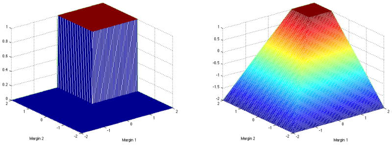
Left panel: the nonsmooth indicator function 1(Z₁ > 0, Z₂ > 0); Right panel: the smooth concave surrogate min(Z₁ − 1, Z₂ − 1, 0) + 1.

This smooth surrogate is shown on the right hand side of Figure 1. We drop the constant 1 in ψ(Z₁, Z₂), since it does not affect the optimization procedure.

Consequently, the SOWL estimator maximizes

$$n^{-1}\sum _{i=1}^n\left[\frac{({\sum }_{j=1}^2{R}_{ij})\psi (A_{i1}{f}_1(H_{i1}),A_{i2}{f}_2(H_{i2}))}{{\prod }_{j=1}^2{\pi }_j(A_{ij},H_{ij})}\right]-{\lambda }_n({\Vert f_1\Vert }^2+{\Vert f_2\Vert }^2),$$ (2.6)

where λ_n is a tuning parameter controlling the amount of penalization. To maximize (2.6), we first restrict to linear decision rules of the form f_j(H_j) = 〈 β_j, H_j 〉 + β_0j for j = 1, 2. The norms of f₁ and f₂ in (2.6) are given by the Euclidean norm of β₁ and β₂. To ease notation, we write $(R_1+R_2)/{\prod }_{j=1}^2{\pi }_j(A_j,H_j)$ simply as W. Thus the optimization problem can be written as

$$max\gamma \sum _{i=1}^n{W}_i{\xi }_i-{\Vert {\beta }_1\Vert }^2-{\Vert {\beta }_2\Vert }^2$$

subject to, ξ_i ≤ 0, ξ_i ≤ A_i1(〈 β₁, H_i1 〉 + β₀₁) − 1, ξ_i ≤ A_i2(〈 β₂, H_i2 〉 + β₀₂) − 1, where γ is a constant depending on λ_n. This optimization problem is a quadratic programming problem with a quadratic objective function and linear constraints. Applying the derivations given in the supplementary material, the dual problem is given by

$$\underset{{\alpha }_1,{\alpha }_2}{max}\sum _{i=1}^n({\alpha }_{i1}+{\alpha }_{i2})-\frac{1}{2}\sum _{i=1}^n\sum _{l=1}^n\sum _{j=1}^2{\alpha }_{ij}{\alpha }_{lj}{A}_{ij}{A}_{lj}\langle H_{ij},H_{lj}\rangle$$

subject to α_i1, α_i2 ≥ 0, ${\sum }_{i=1}^n{\alpha }_{i1}{A}_{ij}=0,{\sum }_{i=1}^n{\alpha }_{i2}{A}_{i2}=0$, α_i1 + α_i2 ≤ γW_i, i = 1, …, n. Hence, the dual problem can be optimized using standard software. Similarly, we may introduce nonlinearity by using nonlinear kernel functions and the associated RKHS. In this case, 〈 H_ij, H_lj 〉 in the dual problem is replaced by the inner product in the RKHS.

To extend SOWL to T stages, where T > 2, we need to find a concave proxy function for the indicator I(Z₁ > 0, …, Z_T > 0), where Z_j = A_jf_j(H_j), j = 1, …, T. A natural generalization of surrogate reward is ψ(Z₁, …, Z_T) = min(Z₁ −1, …, Z_T −1, 0)+1, and the objective function analogous to (2.6) for optimization follows correspondingly. The dual problem and optimization routine can be developed in the same fashion.

3 Theoretical Results

In this section, we present the theoretical results for the methods described in Section 2. Since the best rule at the current stage depends on the best rules at future stages, the theoretical properties of the proposed methods have to be established stage by stage conditioning on the estimated rule at future stages. We first derive the exact form of the optimal DTR. We then provide asymptotic results for using BOWL and SOWL to estimate the optimal DTR.

Define for t = 1, …, T,

$$V_t(f_t,\dots ,f_T)=E\left[\frac{({\sum }_{j=t}^T{R}_j){\prod }_{j=t}^{T}I(A_j=\text{sign}(f_j(H_j)))}{{\prod }_{j=t}^T{\pi }_j(A_j,H_j)}\right].$$ (3.1)

Thus V_t(f_t, …, f_T) is the average total reward gain from stage t until the last stage if the sequence of decisions (sign(f_t), …, sign(f_T)) is followed thereafter. If t = 1, the subscript is dropped, indicating that the value function is calculated for all stages, i.e., V^d = V(f₁, …, f_T) with d = (sign(f₁), …, sign(f_T)). We also define $V_t^{\ast }={sup}_{(f_t,\dots ,f_T)}{V}_t(f_t,\dots ,f_T)$, where supremum is taken over all measurable functions, and $V_t^{\ast }$ is achieved at ( $f_t^{\ast },\dots ,f_T^{\ast }$).

3.1 Fisher Consistency

Fisher consistency states that the population optimizer in BOWL and SOWL is the optimal DTR. Specifically, we show that either by replacing the 0–1 loss with the hinge loss in the target function (2.3) and solving the resulting optimization problem over all measurable functions with the surrogate loss backwards, or by maximizing the surrogate reward with the ψ function replacing the product of 0–1 reward functions in (2.1), we obtain a sequence of decision rules that is equivalent to the optimal DTR.

Proposition 3.1. (BOWL)

If we obtain a sequence of decision functions (f̃₁, …, f̃_T) by taking the supremum over × × … × of

$$E\left[\frac{\left({\sum }_{j=t}^T{R}_j\right){\prod }_{j=t+1}^{T}I(A_j=\text{sign}({\stackrel{\sim }{f}}_j(H_j)))}{{\prod }_{j=t}^T{\pi }_j(A_j,H_j)}\varphi (A_t{f}_t(H_t))\right]$$

backwards through time for t = T, T − 1, …, 1, then $d_j^{\ast }(h_j)=\text{sign}({\stackrel{\sim }{f}}_j(h_j))$ for all j = 1, …, T.

The proof follows by noting that each step is a single-stage outcome weighted learning problem; Zhao et al. (2012) proved that the derived decision rule based on the hinge loss also minimizes 0–1 loss. Therefore, $d_T^{\ast }=\text{sign}({\stackrel{\sim }{f}}_T)$. Given this fact, we obtain $d_{T-1}^{\ast }=\text{sign}({\stackrel{\sim }{f}}_{T-1})$ and so on. This theorem validates the usage of the hinge loss in the implementation, indicating that the BOWL procedure targets the optimal DTR directly. Similarly, the surrogate reward in SOWL has the correct target function. Define

$$V_{\psi }(f_1,\dots f_T)=E\left[\frac{({\sum }_{j=1}^T{R}_j)\psi (A_1{f}_1(H_1),\dots ,A_T{f}_T(H_T))}{{\prod }_{j=1}^T{\pi }_j(A_j,H_j)}\right].$$ (3.2)

The following result is proved in the Appendix.

Proposition 3.2. (SOWL)

If (f̃₁, …, f̃_T) ∈ × … × maximize V_ψ(f₁, …, f_T) over × … × , then for h_j ∈ , $d_j^{\ast }(h_j)=\mathit{sign}({\stackrel{\sim }{f}}_j(h_j))$, j = 1, …, T.

3.2 Relationship between excess values

The maximal V_ψ-value is defined as $V_{\psi }^{\ast }={sup}_{(f_1,\dots ,f_T)}\{V_{\psi }(f_1,\dots ,f_T)\mid f_j\in {\mathcal{F}}_j,j=1,\dots ,T\}$, which is shown in Proposition 3.2 to be maximized at ( $f_t^{\ast },\dots ,f_T^{\ast }$). We have the following result.

Theorem 3.3. (SOWL)

For any f_j ∈ , j = 1, …, T, we have

$$V(f_1^{\ast },\dots ,f_T^{\ast })-V(f_1,\dots ,f_T)\le (1+(T-1)c_0^{-1})[V_{\psi }(f_1^{\ast },\dots ,f_T^{\ast })-V_{\psi }(f_1,\dots ,f_T)],$$

where ( $f_1^{\ast },\dots ,f_T^{\ast }$) is the optima over × … × .

Theorem 3.3 shows that the difference between the value for (f₁, …, f_T) and the optimal value function with 0–1 rewards is no larger than that under the surrogate reward function ψ multiplied by a constant. This quantitative relationship implies a relationship between excess values for V(f₁, …, f_T) and V_ψ(f₁, …, f_T), which is particularly useful in the sense that if the V_ψ value of certain decision rules is fairly close to $V_{\psi }^{\ast }$, the decision rules also yield a nearly optimal value.

Remarks

Similar properties for one-dimensional hinge loss have been derived when optimizing over an unrestricted function class (see Bartlett et al., 2006; Zhao et al., 2012), where the relationship between excess risk associated with 0–1 loss is always bounded by that associated with hinge loss. Since each step is a single-stage outcome weighted learning, we naturally obtain the analogous results for BOWL at each stage and do not elaborate here.

3.3 Consistency, risk bound and convergence rates

As indicated in Sections 2.3 and 2.4, the estimation of optimal DTR occurs within a specific RKHS. We obtain linear decision rules using linear kernels for the RKHS and nonlinear decision rules with nonlinear kernels. Propositions S.1 and S.2 in the supplementary material show that, as sample size increases, if the optimal DTR, which is obtained by taking the supremum over all measurable functions, belongs to the closure of the selected function space, the value of the estimated regimes via BOWL or SOWL will converge to the optimal value. Note that Q-learning does not guarantee this kind of property. If any of the postulated regression models are misspecified, Q-learning may be inconsistent for the optimal DTR even if it is contained within the class of DTRs induced by the Q-functions.

We now derive the convergence rate of $V_j({\widehat{f}}_j,\dots ,{\widehat{f}}_T)-V_j^{\ast }j=T$, T − 1, … 1 for the BOWL estimator and V(f̂₁, …, f̂_T) − V^* for the SOWL estimator. We particularly consider the RKHS , j = t, …, T, as the space associated with Gaussian Radial Basis Function (RBF) kernels $k_j(h_j,h_j^{\prime })=exp(-{\sigma }_{j,n}^2{\Vert h_j-h_j^{\prime }\Vert }^2),h_j,h_j^{\prime }\in {\mathcal{O}}_j$, and σ_j,n > 0 is a parameter varying with n controlling the bandwidth of the kernel. Therefore, when conducting BOWL backwards and at each stage or SOWL simultaneously, we will encounter two types of error: approximation error, representing the bias by comparing the best possible decision function in with that across all possible spaces, and estimation error, reffecting the variability from using a finite sample. In order to bound estimation error, we need a complexity measure for the selected space. Here, by using the Gaussian RBF kernel, the covering number for can be controlled via the empirical L₂-norm, defined as ${\Vert f_j-g_j\Vert }_{L_2(P_n)}={({\sum }_{i=1}^n\mid f_j(H_{ij})-g_j(H_{ij}){\mid }^2/n)}^{1/2}$. Specifically, for any ε > 0, the covering number of a functional class with respect to L₂(P_n), N ( , ε, L₂(P_n)), is the smallest number of L₂(P_n) ε-balls needed to cover where an L₂(P_n) -ball around a function g ∈ is the set {f ∈ : ||f − g||_L2(Pn) < ε}. We assume that at stage j,

$$\underset{P_n}{sup}logN(B_{{\mathcal{H}}_{k_j}},\epsilon ,L_2(P_n))\le c_{\nu ,\delta ,p_j}{\sigma }_{j,n}^{(1-\nu /2)(1+\delta )p_j}{\epsilon }^{-\nu },$$

where is the closed unit ball of , and ν and δ are any numbers satisfying 0 < ν ≤ 2 and δ > 0. To determine the approximation properties of Gaussian kernels, we assume a geometric noise condition regarding the distribution behavior of data near the true decision boundary at each stage, which has been used to derive the risk bounds for SVMs (Steinwart and Scovel, 2007) and for single stage value maximization (Zhao et al., 2012). For each stage j, the noise exponent q_j reffects the relationship between magnitude of the noise and the distance to the decision boundary. Details on the noise condition are provided in the supplementary material.

Theorem 3.4. (BOWL)

Let the distribution of (H_j, A_j, R_j), j = 1, …, T satisfy Condition S.1 in the supplementary material with noise exponent q_j > 0. Then for any δ > 0, 0 < ν ≤ 2, there exists a constant K_j (depending on ν, δ, p_j and π_j), such that for all τ ≥ 1, π_j(a_j, h_j) > c₀ and ${\sigma }_{j,n}={\lambda }_{j,n}^{-1/(q_j+1)p_j}$, j ≥ t, ${Pr}^{\ast }\left(V_t({\widehat{f}}_t,\dots ,{\widehat{f}}_T)\ge V_t^{\ast }-{\sum }_{j=t}^T{(3^{-1}{c}_0)}^{t-j}{\epsilon }_j\right)\ge 1-{\sum }_{j=t}^T{2}^{j-t}{e}^{-\tau }$, where Pr^* denotes the outer probability for possibly nonmeasurable sets, and

$${\epsilon }_j=K_j\left[{\lambda }_{j,n_j}^{-\frac{2}{2+\nu }+\frac{(2-\nu )(1+\delta )}{(2+\nu )(1+q_j)}}{n}_j^{-\frac{2}{2+\nu }}+\frac{\tau }{n_j{\lambda }_{j,n_j}}+{\lambda }_{j,n_j}^{\frac{q_j}{q_j+1}}\right],$$ (3.3)

where n_j is the available sample size at stage j. Particularly, when t = 1, we have ${Pr}^{\ast }\left(V^{\widehat{\mathbf{d}}}\ge V^{\ast }-{\sum }_{j=1}^T{(3^{-1}{c}_0)}^{1-j}{\epsilon }_j\right)\ge 1-{\sum }_{j=1}^T{2}^{j-1}{e}^{-\tau }$.

Theorem 3.5. (SOWL)

Let the distribution of (H_j, A_j, R_j), j = 1, …, T with noise exponent q_j > 0. Then for any δ > 0, 0 < ν < 2, there exists a constant K (depending on ν δ, p_j and π_j), such that for all τ ≥ 1 and ${\sigma }_{j,n}={\lambda }_{j,n}^{-1/(q_j+1)p_j}$, Pr^*(V(f̂₁, …, f̂_T) ≥ V^* − ε) ≥ 1 − e^−τ, where

$$\epsilon =K\left[{\lambda }_n^{-\frac{2}{2+\nu }}{\left(\sum _{j=1}^T{\lambda }_n^{\frac{(2-\nu )(1+\delta )}{2+2q_j}}\right)}^{\frac{2}{2+\nu }}{n}^{-\frac{2}{2+\nu }}+\frac{\tau }{n{\lambda }_n}+\sum _{j=1}^T{\lambda }_n^{\frac{q_j}{q_j+1}}\right].$$ (3.4)

Theorems 3.4 and 3.5 measure the probability that the difference between the value of the estimated DTR using BOWL or SOWL and the optimal value is sufficiently small. Specifically for BOWL, we bound the difference between the value of the estimated DTRs starting at arbitrary stage t and the optimal value from that stage on. Furthermore, we can derive the rate of convergence of the estimated values approaching the corresponding targeted optimal values. Each ε_j, j = 1, …, T in (3.3), as well as ε in (3.4), consists of the estimation error, the first two terms, and the approximation error, the last term. In particular, if q_j = q (j = 1, …, T) and we balance the estimation and approximation error by letting ${\lambda }_{j,n}={n_j}^{-\frac{2(1+q)}{(4+\nu )q+2+(2-\nu )(1+\delta )}}$ in (3.3) or (3.4), then the optimal rate for the value of the estimated DTRs using BOWL or SOWL is $O_p(n_1^{-\frac{2q}{(4+\nu )q+2+(2-\nu )(1+\delta )}})$. In this formula, δ is a free parameter which can be set arbitrarily close to 0. The geometric noise component q is related to the noise condition regarding the separation between two optimal treatment groups. The parameter ν measures the order of complexity for the associated RKHS. For example, if the two subsets ${\mathcal{O}}_j^{+}$ and ${\mathcal{O}}_j^{-}$, j = 1, …, T have strictly positive distance, i.e., there is no data near the decision boundary across all stages, then q = ∞ and the convergence rate is approximately $n_1^{-1/(2+\nu )}$, and $n_1^{-1/2}$ with ν close to 0.

Remarks

The fast rate of convergence to the best achievable error for SVMs is anticipated provided certain conditions hold on the data generating distribution (Tsybakov, 2004; Steinwart and Scovel, 2007; Blanchard et al., 2008). Indeed, the convergence rate of $n_1^{-1/2}$ can be further improved to as fast as $n_1^{-1}$ if η_j(h_j), j = 1, …, T are bounded away from 1/2 by a gap, that is, there is a distinction between the rewards gained from treatment 1 and −1 on the same patient. More details can be found in the supplementary material.

4 Simulation Studies

To assess the performance of the proposed methods, we conduct simulations under a number of scenarios imitating a multi-stage randomized trial. We first consider a two-stage setup. Specifically, 50 dimensional baseline covariates X_1,1, …, X_1,50 are generated according to N (0, 1). Treatments A₁, A₂ are randomly generated from {−1, 1} with equal probability 0.5. The models for generating outcomes R₁ and R₂ vary under the different settings stated below:

• 1Stage 1 outcomeR₁ is generated according to N (0.5X_1,3A₁, 1), and stage 2 outcome R₂ is generated according to $N(((X_{1,1}^2+X_{1,2}^2-0.2)(0.5-X_{1,1}^2-X_{1,2}^2)+R_1)A_2,1)$.
• 2Stage 1 outcomeR₁ is generated according to N ((1 + 1.5X_1,3)A₁, 1); two intermediate variables, X_2,1 ~ I{N (1.25X_1,1A₁, 1) > 0}, and X_2,2 ~ I{N (−1.75X_1,2A₁, 1) > 0} are generated; then the Stage 2 outcome R₂ is generated according to N ((0.5 + R₁ + 0.5A₁ + 0.5X_2,1 − 0.5X_2,2)A₂, 1).

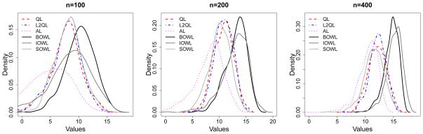
There are no time-varying covariates involved in Scenario 1, and a non-linear relationship exists between baseline covariates and stage 2 treatment. Additionally, R₁ plays a role in determining the second stage outcomes. We incorporate two time-varying covariates in Scenario 2, i.e., additional binary covariates are collected after stage 1, the values of which depend on the first and second baseline variables. In the third scenario, we consider a three-stage SMART with data generated as follows.

• 3Treatments A₁, A₂ and A₃ are randomly generated from {−1, 1} with equal probability 0.5. Three baseline covariates X_1,1, X_1,2, X_1,3 are generated with N (45, 15²). X₂ is generated according to X₂ ~ N (1.5X_1,1, 10²) and X₃ is generated according to X₃ ~ N (0.5X₂, 10²). R_j = 0, j = 1, 2 and R₃ ~ 20 − |0.6X_1,1 − 40|{I(A₁ > 0) − I(X_1,1 > 30)}² − |0.8X₂ − 60|{I(A₂ > 0) − I(X₂ > 40)}² − |1.4X₃ − 40|{I(A₃ > 0) − I(X₃ > 40)}².

In this scenario, the regret for stage 1 is |0.6X₁ − 40|{I(A₁ > 0) − I(X_1,1 > 30)}², the regret for stage 2 is given by |0.8X₂ − 60|{I(A₂ > 0) − I(X₂ > 40)}² and the regret for stage 3 is given by |1.4X₃ − 40|{I(A₃ > 0) − I(X₃ > 40)}². We can easily obtain the optimal decision rule by setting the regret to zero at each stage. That is, $d_1^{\ast }(h_1)=\text{sign}(x_{1,1}-30),d_2^{\ast }(h_2)=\text{sign}(x_2-40)$, and $d_3^{\ast }(h_3)=\text{sign}(x_3-40)$. In the simulations, we vary sample sizes from 100, 200 to 400 and repeat each scenario 500 times.

For each simulated data set, we apply the proposed learning methods including BOWL, IOWL, and SOWL. We also implement the Q-learning, L₂-regularized Q-learning, and A-learning for the purpose of comparison. In all these algorithms, we consider linear kernels for illustration. We also explored the use of Gaussian kernels but found that the performance changed little in any of these scenarios. In order to carry out Q-learning, we consider a linear working model for the Q-function of the form Q_j(H_j, A_j; α_j, γ_j) = α_jH_j + γ_jH_jA_j, j = 1, …, T, where H₁ = (1, X₁), and H_j = (H_j−1, H_j−1A_j−1, X_j) and X_j includes R_j−1 and other covariates measured after A_j−1. Here we assume H_j includes intercept terms. Take T = 2 as the example, the second stage parameter can be estimated as $({\widehat{\alpha }}_2,{\widehat{\gamma }}_2)={\text{argmin}}_{{\alpha }_2,{\gamma }_2}{\sum }_{i=1}^n{(R_{i2}-Q_2(H_{i2},A_{i2};{\alpha }_2,{\gamma }_2))}^2$, and the estimated treatments for stage 2 are obtained via argmax_a2 Q₂(H₂, a₂; α̂₂, γ̂₂). We then obtain pseudo outcomes for stage 1 with R̂₁ = R₁ + max_a2 Q₂(H₂, a₂; α̂₂, γ̂₂). (α̂₁, γ̂₁) can be computed by fitting the imposed model Q₁(H₁, A₁; α₁, γ₁) for R̂₁, and the estimated stage 1 treatments are argmax_a1 Q₁(H₁, a₁; α̂₁, γ̂₁). L₂-regularized Q-learning is considered to handle the high dimensional covariate space, where ridge regression with an L₂ penalty is applied at each stage. The regularization parameter was chosen using cross validation. We implement A-learning using an iterative minimization algorithm developed in Murphy (2003), where the regret functions are linearly parameterized with other components unspecified. For BOWL, we follow the procedures described in Section 2.3, where the optimal second stage treatments are obtained via a weighted SVM technique based on history H₂, with the optimization target defined in (2.4). The estimation of the optimal treatment in stage 1 is then carried out by minimizing (2.5) using H₁ on the subset of patients whose assignments A₂ are consistent with the estimated decisions d̂₂. The weighted SVM procedure is implemented using LIBSVM (Chang and Lin, 2011). We use 5-fold cross validation to select tuning parameters λ_t,n in each stage: the data is partitioned into 5 subsets; each time 4 subsets are used as the training data for DTR estimation while the remaining set is used as the validation data for calculating the value of the estimated rule; the process is repeated 5 times and we average the value obtained each time; then we choose λ_t,n for stage t, to maximize the estimated values. In the IOWL method, we iteratively apply the weighted SVM technique, based on the group of patients receiving the recommended treatment for the other stage. Again, cross validation is utilized to select the required tuning parameter via a grid search. The iterative procedure stops upon stabilization of the value functions or reaching the maximum number of iterations, preset in our simulations. In the implementation of SOWL, we maximize the objective function presented in (2.6) coupled with a commonly used procedure in convex optimization (Cook, 2011), where the parameter λ_n is chosen via 5-fold cross-validation. In general, it takes less than 1 minute to run a 2-stage example, and 3 minutes to run a 3-stage example, where we select tuning parameters for each stage based on a prefixed set of 15 candidate values, on a Macbook Pro with CPU 2.6 GHz Intel Core i7, 16GB memory.

Scientific interest is to investigate the ability of the estimated DTRs to produce an optimal outcome. In each scenario, based on one training set out of 500 replicates, we construct DTRs using competing methods. For each estimated DTR, we calculate the mean response had the whole population followed the rule (the value function) by Monte Carlo methods. Specifically, we generate a large validation data set (size 10000) and obtain the subject outcomes under the estimated DTRs. Therefore, the values of the value function can be calculated by averaging the outcomes over 10000 subjects, and we have 500 values of the estimated rules on the validation set for each scenario. We summarize the results by plotting the smoothed histograms of these values obtained, which are displayed in Figures 2{4. We expect to see better performing methods leading to large values more frequently. We also provide means and standard errors (s.e.) of the values over 500 runs for each scenario in Table 1.

Figure 2.

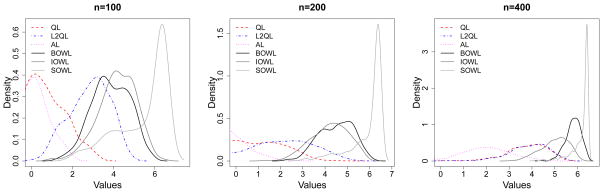
Smoothed Histograms of Values of Estimated DTRs for Scenario 1. The optimal value is V^* = 6.695.

Figure 4.

Smoothed Histograms of Values of Estimated DTRs for Scenario 3. The optimal value is V^* = 20.

Table 1.

Mean values of the estimated DTR for Scenarios 1–3

	n	Q-learning	L2Q-learning	A-learning	BOWL	IOWL	SOWL
Scenario 1	100	0.692 (0.972)	2.831 (0.972)	−0.298 (0.984)	3.849 (0.918)	4.166 (0.921)	5.428 (1.234)
	200	0.583 (1.476)	1.928 (1.533)	−0.650 (0.991)	4.502 (0.768)	4.210 (0.840)	5.933 (0.755)
	400	3.766 (0.896)	3.859 (0.897)	1.973 (1.072)	5.811 (0.331)	4.996 (0.602)	6.189 (0.388)
Scenario 2	100	1.462 (0.361)	2.857 (0.248)	0.369 (0.318)	2.709 (0.340)	2.777 (0.314)	3.026 (0.141)
	200	1.122 (0.679)	2.650 (0.547)	0.631 (0.322)	2.847 (0.269)	2.871 (0.278)	3.119 (0.084)
	400	3.435 (0.041)	3.449 (0.043)	2.549 (0.394)	3.105 (0.131)	3.049 (0.197)	3.212 (0.089)
Scenario 3	100	7.633 (2.953)	7.765 (2.669)	2.184 (6.377)	10.231 (2.563)	8.378 (3.854)	8.192 (2.359)
	200	10.762 (1.846)	10.86 (1.676)	7.454 (4.083)	13.139 (1.952)	12.978 (2.457)	10.08 (1.957)
	400	12.105 (1.605)	12.204 (1.419)	10.495 (1.882)	14.617 (1.299)	15.120 (1.443)	11.533 (1.788)

With large number of covariates, Q- and A-learning tend to overfit the model, leading to worse performances in general. L₂-regularized Q-learning yields an improvement, yet the performance is not satisfactory when the treatment effect is misspecified. For example, the treatments effect is highly nonlinear in Scenario 1, where a linear basis is used for modeling. In this situation, Q- and A-learning based methods may never closely approximate the correct decision boundary. As shown in Figure 2, they tend to estimate the wrong target since the mean of the distribution deviates from the optimal value substantially. Even though the proposed methods also misspecify the functional relationship, they outperform Q-learning/A-learning, and behaviors of the three methods are consistent in the sense that different approaches most of the time lead to the same value, which is close to the truth. Scenario 2 takes evolving variables into consideration and responses generated at each stage are linearly related to the covariates. Again, the proposed methods are comparable or better than Q- and A-learning. In Scenario 3, we mimic a 3-stage SMART. This imposes significant challenges on deriving the optimal DTRs due to limited sample sizes yet multiple options of treatment sequences over 3 stages. Although the optimal treatment decision at each stage is linear, the Q-function and the regret function are not linear here. Hence, the posited models in Q-learning and A-learning are misspecified, but the proposed methods using linear kernel are correct. Indeed, the proposed methods have better performances for this complex scenario, and the values of the deduced DTRs are closer to the optimal value as sample size increases. The strength of IOWL over BOWL is demonstrated in this example. By taking advantage of an iterative process cycling over the complete data set, it improves the decision from BOWL with better precision. In addition to Q- and A-learning, Zhang et al. (2013) proposed a robust method to search for the optimal DTRs within a pre-specified treatment class using a genetic algorithm. Since their method cannot handle very high-dimensional covariate spaces, we perform comparisons by keeping only key covariates in the simulation, with the data generation mechanism remaining the same. When the number of predictors is reduced, all methods tend to perform similarly, and ones with modeling assumptions satisfied can have comparatively better performances (see Table S.2 in the supplementary material). Additional simulation results are also presented in the supplementary materials, including settings with simple treatment effects and discrete covariates. The proposed methods have comparable or superior performances to all competing approaches.

5 Data Analysis: Smoking Cessation Study

In this section we illustrate the proposed methods using data from a two-stage randomized trial of the effectiveness of a web-based smoking intervention (see Strecher et al., 2008, for details). The smoking cessation study consists of two stages. The purpose of stage 1 of this study (Project Quit), was to find an optimal multicomponent behavioral intervention to help adult smokers quit smoking; and among the participants of Project Quit, the subsequent stage (Forever Free) was conducted to help those who already quit stay quit, and help those who failed to quit continue the quitting process. The study initially enrolled 1848 patients of which only 479 continued on to the second stage.

The baseline covariates considered in stage 1 include 8 variables, denoted by X_1,1, …, X_1,8, and 2 additional intermediate variables, X_2,1 and X_2,2, measured after 6 months are considered in stage 2. Both of them are described in the supplementary material. The first stage treatment is A₁ = “Story” which dictates the tailoring depth of a web-based intervention. “Story” is binary and is coded 1 and −1 with 1 corresponding to high tailoring depth (more tailored) and −1 corresponding to low tailoring depth (less tailored). The second stage treatment is A₂=“FFArm” which is also binary and coded as −1 and 1, with −1 corresponding to control and 1 corresponding to active treatment. A binary outcome was collected at 6 month from stage 1 randomization, with R_Q1 = 1 if the patients quit smoking successfully and 0 otherwise. The stage 2 outcome was collected as R_Q2 (1 = quit, 0 = not quit) from stage 2 randomization. To simplify our analysis, we first only consider the subset of patients that completed both stages of treatment with complete covariate and corresponding outcome information.

We are mainly interested in examining the performance of the proposed approaches, i.e., BOWL, IOWL and SOWL. However, to serve as a baseline we also consider Q-learning and A-learning as competitors. For the implementation of Q-learning, we need to posit a model for each decision point. We first incorporate all the history covariates and history-treatment interactions, i.e., H₁ = (1, X₁) and H₂ = (H₁, H₁A₁, X_2,1, X_2,2, R₁), into the prediction models for Q-functions. A-learning is implemented with H_j as linear predictors for the contrast at stage j, j = 1, 2. For BOWL, IOWL and SOWL methods, linear kernels are considered with H_j as input for both stage, j = 1, 2. We use R_Qj divided by the estimated π̂_j(a_j, H_j), where π̂_j(a_j, H_j) = Σ_j I(A_j = a_j)/n_j to weigh each subject, and n_j is the sample size at stage j.

For any DTR d = (d₁, d₂), we can estimate the associated value using

$${\widehat{V}}^{\mathbf{d}}=\frac{{\mathbb{E}}_n\left[(R_{Q1}+R_{Q2})I(A_1=d_1(H_1),A_2=d_2(H_2))/{\prod }_{j=1}^2{\widehat{\pi }}_j(A_j,H_j)\right]}{{\mathbb{E}}_n\left[I(A_1=d_1(H_1),A_2=d_2(H_2))/{\prod }_{j=1}^2{\widehat{\pi }}_j(A_j,H_j)\right]}.$$

Let’s first consider non-dynamic regimes. If the entire patient population follows the fixed regime d = (1, 1), i.e., stories are highly tailored to the whole population in stage 1, and all patients are provided with treatment in the second stage, the expected value associated with (1, 1) is 0.729. Similarly, we have V̂^{(1, −1)} = 0.878, V̂^(−1,1) = 0.769 and V̂^{(−1, −1)} = 0.568. Using the complete dataset, we derive the DTRs based on different methods. The values for the derived treatment regimes can also be estimated unbiasedly using the same strategy. In general, the use of estimated optimal DTRs, which are tailored to individual characteristics, yield better outcomes than any fixed treatment regimes. The highest value results from regimes recommended by BOWL, with V̂^d̂_BOWL = 1.096, followed by the regimes recommended from IOWL with V̂^d̂_IOWL = 1.019. Fewer patients follow the regime (1, 1), while around half of the patients are recommended with the regime (1, −1). By checking the loadings of the covariates in the estimated rules using BOWL methods, we find that people with lower motivation to quit smoking should more frequently be assigned to highly tailored stories. We also learn that smokers who quit smoking but with lower self-efficacy after stage 1 should be recommended to active treatment at the second stage. Results from the considered methods are presented in Figure 5 for comparison. We can see that the proposed methods provide similar recommendations, which lead to better benefits compared with other methods.

Figure 5.

Selected Percentages of Two-Stage Treatments using Different Methods

Note: The estimated values using different methods are: 0.835 by Q-learning (QL), 0.863 by L₂Q-learning (L2QL), 0.933 by A-learning (AL), 1.096 by BOWL, 1.019 by IOWL and 0.999 by SOWL. Stage 1 treatment denoted by 1 or −1 represents a highly tailored story or the opposite. Stage 2 treatment denoted by 1 or −1 indicates a treatment or not.

Indeed, there is considerable dropout during the study. We may possibly introduce bias by doing a complete-case data analysis as above. Here, we present one possible remedy yet not necessarily the best approach by including dropout within the reward structure, since to handle missing data appropriately, one would hope to have a full understanding of the missing mechanism. Among dropout patients, 317 patients quit smoking successfully and 601 did not. We adopted the principle of last observation carried forward, i.e., for each dropout subject, we impute R_Q2 by the observed R_Q1 for the same subject. Hence, the outcome of interest is 2R_Q1 for patients not moving into stage 2, and (R_Q1 + R_Q2) otherwise. We apply Q-learning, BOWL and IOWL to the dataset under this framework, which yield values of 0.742, 0.787 and 0.779 accordingly. BOWL produces a better strategy, where by checking the loadings of the covariates in the estimated BOWL rule, we find that people with lower motivation to quit smoking or lower education level (≤ high school) should be provided with highly tailored stories.

Considering the potential problems arising from overfitting, we further perform a cross-validation type analysis using complete-case data. For 100 iterations we randomly split the data into 2 roughly equally sized parts, one part of the data is used as a training set, on which the methods are applied to estimate the optimal DTR, and the remaining part is retained for validation by calculating values of the obtained estimates. Moreover, we consider two additional outcomes for the purpose of a comprehensive comparison: a binary outcome R_Sj = 1 if the level of satisfaction with the smoking cessation program is high and R_Sj = 0 otherwise, j = 1, 2; and ordinal outcomes R_Nj= 0 if the patient had zero abstinent months; R_Nj = 1 if the patient experienced 1–3 abstinent months; and R_Nj = 2 if the patient experienced 4 or more abstinent months during the j^th stage. Table 2 gives the mean and the standard error of the cross validated values across 100 iterations for different outcomes, where higher values signify better results. It can be seen that values resulted from BOWL/IOWL/SOWL for all outcomes are comparable or higher than either Q- or A-learning. One possible reason for this is that the proposed methods do not attempt to do model fitting. Q- or A-learning impose regression models, particularly linear here, for the Q-function or regret function, which may be misspecified.

Table 2.

Mean (s.e.) Cross Validated Values using Different Methods

	Mean (s.e.) Cross Validated Values
Outcome	BOWL	IOWL	SOWL	Q-learning	L2Q-learning	A-learning
RQ	0.747 (0.099)	0.768 (0.101)	0.751 (0.073)	0.692 (0.089)	0.696 (0.093)	0.709 (0.090)
RN	1.550 (0.175)	1.534 (0.199)	1.514 (0.158)	1.487 (0.141)	1.565 (0.140)	1.453 (0.151)
RS	1.262 (0.093)	1.288 (0.114)	1.254 (0.091)	1.216 (0.087)	1.231 (0.094)	1.183 (0.084)

6 Discussion

We have proposed novel learning methods to estimate the optimal DTR using data from a sequential randomized trial. The proposed methods, formulated in a nonparametric framework, are computationally efficient, easy and intuitive to apply, and can effectively handle the potentially complex relationships between sequential treatments and prognostic or intermediate variables.

All three of the proposed estimators are philosophically similar in that they aim to maximize the value function directly, and yield a unique optima which converges to the true optimal value asymptotically. However, they use different optimization methods to find the optimal DTR – backward recursion for BOWL and IOWL, simultaneous optimization for SOWL. This simultaneous optimization may cause some numerical instability in SOWL when the number of stages is large. Comparatively, BOWL and IOWL may have more benefits in the complex setting with multiple (>2) stages. While we primarily considered SVMs in this paper, this is not essential, and any classification algorithm capable of accommodating example weights could be used, e.g., tree-based methods, neural networks, etc. In fact, one could use different classification algorithms at each stage. Conversely, SOWL attempts a simultaneous estimation of the decision rules at each stage by using a single concave relaxation of the empirical value function. Furthermore, a new algorithm is developed to facilitate optimization over multiple stages simultaneously. This relaxation involves defining a multi-dimensional analog of the margin in classification and a corresponding multi-dimensional hinge-loss. However, since such methods have not yet been widely studied (to our knowledge, this is the first time such an approach has been used) questions of how to choose an effective concave relaxation for a given problem as well as how best to tune such a relaxation remain open questions. We assume the R_j to be non-negative, and suggest to replace R_j by R_j − min_i R_ij if any of the observed values are negative. The shift in location does not affect the method’s asymptotic properties, but it may have some impact in finite samples. We are currently investing this issue to examine some optimal recoding of rewards when they are not all nonnegative.

The proposed methods enjoyed improved empirical performance when compared with regression based methods Q- and A-learning. One reason for this is that the proposed methods directly estimate the optimal DTR rather than attempting to back it out of conditional expectations. There is a direct analogy between hard- and soft-margin classifiers wherein hard-margin classifiers directly estimate the decision boundary and soft-margin classifiers back-out the decision boundary through conditional class probabilities. When the class probabilities are complex, hard-margin classifiers may lead to improved performance (Wang et al., 2008); likewise, when the conditional expectations are complex, directly targeting the decision rule is likely to yield improved performance. Since the proposed methods do not model the relationship between outcomes and DTRs, they may be more robust to model misspecification than statistical modeling alternatives such as Q-learning (Zhang et al., 2012b,a). Modeling based approaches may be more efficient if the model is correctly specified. In the multi-decision setup, to find the best rule at one stage, we need to take into account the future rewards assuming that the optimal treatment regimes have been followed thereafter. Using a nonparametric approach, we cannot use the information from the patients whose assigned treatments are different from the optimal ones, since the observed rewards underestimate the true optimal future rewards. With modeling step included, Q-learning can impute the predicted future outcomes for constructing optimal DTRs. We may consider integrating both approaches by predicting the missing outcomes via Q-learning and subsequently estimating the optimal DTRs via IOWL/BOWL/SOWL. This would allow us to combine the strengths of both methods and potentially obtain more refined results in decision making and future prediction.

Sometimes, more than two treatments are available; an extreme example includes optimal dosing where there are a continuum of treatments. Hence, extensions to multiple and continuous treatments are needed. Existing methods for multi-category classification can be used with the proposed methodology to handle the multiple treatments case (Liu and Yuan, 2011). For continuous treatments, one possibility is to smooth over treatments, such as replacing indicators with kernel smoothers. In addition, methods for estimating DTRs should be developed which are capable of operating effectively within ultra-high dimensional predictor spaces. A possible solution under the proposed framework is to incorporate sparse penalties in the optimization procedure, for example, the l₁ penalty (Bradley and Mangasarian, 1998; Zhu et al., 2003).

It is critical to recognize that the presented approaches are developed for the discovery of optimal DTRs. In contrast to typical randomized clinical trials, which are conducted to confirm the efficacy of new treatments, the SMART designs mentioned at the beginning of this article are devised for exploratory purposes in developing optimal DTRs. However, a confirmatory trial with a phase III structure can be used to follow-up and validate the superiority of the estimated DTR compared to existing therapies. Conducting statistical inference for DTRs is especially important to address questions such as “How much confidence do we have in concluding that the obtained DTR is the best compared to other regimes?” Efforts have been made to construct confidence intervals for the parameters in the Q-function, with main challenges coming from nonregularity due to the non-differentiability of the max operator (Robins, 2004; Chakraborty et al., 2010; Laber et al., 2011). We have shown that the proposed methods lead to small bias in estimating the optimal DTR and derived finite sample bounds for the difference between the expected cumulative outcome using the estimated DTR and that of the optimal one. We believe that this article paves the way for further developments in finding the limiting distribution of the value function and calculating the required sample sizes for the multi-decision problem.

We require in Assumption (b) that the π_j are bounded away from 0 and 1, since the performance of the proposed approach may be unstable with small π_j(A_j, H_j). One fix is to replace π_j(A_j, H_j) by a stabilized weight, for example, one may use π_j(A_j, H_j)/ π_j(−1, H_j) or project π_j(A_j, H_j) onto [c₀, c₁]. The proposed methods and theory still apply. While we only considered data generated from SMART designs here, the proposed methodology can be extended for use with observational data. In this case, π_j is unknown and must be estimated (Rosenbaum and Rubin, 1983), and Assumption (b) may be violated. The framework has to be generalized and/or stronger modeling assumptions have to be made. Another important issue is missing data, for example, as in the smoking cessation trial in Section 5. We provide a strategy to account for missing responses due to patient dropout, yet there may also be item-missingness. Imputation techniques can be used to handle this problem, i.e., impute values for the missing data and conduct the optimal DTR estimation using the imputed values as if they were the truth (Little and Rubin, 2002; Shortreed et al., 2011). Generalization for right-censored survival data is also crucial. Methods have been developed for the multi-decision problem within the Q-learning framework, where survival times are the outcome of interest (Zhao et al., 2011; Goldberg and Kosorok, 2012). Outcome weighted learning approaches, however, have not yet been adapted to handle censored data. It would be worthwhile to investigate the possibility of such a generalization.

Figure 3.

Smoothed Histograms of Values of Estimated DTRs for Scenario 2. The optimal value is V^* = 3.667.

Appendix A. Sketched Proofs

Here we sketch the proofs of theoretical results. For completeness, the details are provided in the supplementary materials (Section S.5). With any DTR d, we associate the sequence of decision functions (f₁, …, f_T) where d_t(h_t) = sign(f_t(h_t)), h_t ∈ for t = 1, −, T. Define the conditional value function for stage t given h_t ∈ as

$$U_t(h_t;f_t,\dots ,f_T)=E\left[\frac{({\sum }_{j=t}^T{R}_j){\prod }_{j=t}^{T}I(A_j=\text{sign}(f_j(H_j)))}{{\prod }_{j=t}^T{\pi }_j(A_j,H_j)}|H_t=h_t\right],t=1,\dots ,T.$$

This conditional value function can be interpreted as the reward gain in the long term given the current history information h_t when using the decision rules (sign(f_t), …, sign(f_T)) thereafter. Let be the set of all measurable functions mapping from to ℝ. Accordingly, we define the optimal value function given h_t at stage t as $U_t^{\ast }(h_t)={sup}_{(f_t,\dots ,f_T)\in {\mathcal{F}}_t\times \dots \times {\mathcal{F}}_T}{U}_t(h_t;f_t,\dots ,f_T)$, achieved at ( $f_t^{\ast },\dots ,f_T^{\ast }$), the optima over all measurable functions on × … × . The optimal decision rule at stage t, $d_t^{\ast }:{\mathcal{O}}_t\to {\mathcal{A}}_t$, can be expressed in terms of $U_t^{\ast }(h_t)$, where

$$d_t^{\ast }(h_t)=\text{sign}(f_t^{\ast }(h_t))=\underset{a_t\in \{-1,1\}}{\text{argmax}}E[R_t+U_{t+1}^{\ast }(H_{t+1})\mid H_t=h_t,A_t=a_t].$$ (6.1)

Note that V_t(f_t, …, f_T) = E(U_t(H_t; f_t, …, f_T)) and $V_t^{\ast }=E(U_t^{\ast }(H_t))$.

Proof of Proposition 3.2

We prove the results for T = 2 while the results for T > 2 can be obtained by induction. According to (6.1), $d_1^{\ast }(h_1)={\text{argmax}}_{a_1\in \{-1,1\}}E(R_1+U_2^{\ast }(H_2)\mid H_1=h_1,A_1=a_1)$, and $d_2^{\ast }(h_2)={\text{argmax}}_{a_2\in \{-1,1\}}E(R_2\mid H_2=h_2,A_2=a_2)$. We need to show that the obtained (f̃₁, f̃₂) by maximizing SOWL objective V_ψ(f₁, f₂) over all measurable functions satisfies, for particular h₁, $d_1^{\ast }(h_1)=\text{sign}({\stackrel{\sim }{f}}_1(h_1))$ and for particular h₂, $d_2^{\ast }(h_2)=\text{sign}({\stackrel{\sim }{f}}_2(h_2))$.

Denote Z_j = A_jf_j(H_j), $Z_j^{\ast }=A_j{f}_j^{\ast }(H_j)$, j = 1, 2. For each h₂ ∈ , A₁ = a₁ and H₁ = h₁ are fixed constants since H₂ = h₂ includes all prior information. Then

$$\begin{array}{l}E\left[\frac{({\sum }_{j=1}^2{R}_j)\psi (Z_1,Z_2)}{{\prod }_{j=1}^2{\pi }_j(A_j,H_j)}|H_2=h_2\right]\\ =E\left(\frac{({\sum }_{j=1}^2{R}_j)min(f_2(h_2)-1,min(a_1{f}_1(h_1)-1,0)))}{{\pi }_1(a_1,h_1)}|H_2=h_2,A_2=1\right)\\ +E\left(\frac{({\sum }_{j=1}^2{R}_j)min(-f_2(h_2)-1,min(a_1{f}_1(h_1)-1,0)))}{{\pi }_1(a_1,h_1)}|H_2=h_2,A_2=-1\right).\end{array}$$

According to Lemma S.1 in the supplementary material, we obtain

$${\stackrel{\sim }{f}}_2(h_2)=\mid 1+min(a_1{f}_1(h_1)-1,0)\mid \text{sign}[E(R_2\mid H_2=h_2,A_2=1)-E(R_2\mid H_2=h_2,A_2=-1)],$$

and thus $d_2^{\ast }(h_2)=\text{sign}({\stackrel{\sim }{f}}_2(h_2))$. Particularly, (f₁, f₂) achieves the maxima where f₂ = f̃₂.

Furthermore, for each h₁ ∈ , to find f̃₁ ∈ , we maximize

$$\begin{array}{l}E\left[\frac{({\sum }_{j=1}^2{R}_j)\psi (Z_1,A_2{\stackrel{\sim }{f}}_2(H_2))}{{\prod }_{j=1}^2{\pi }_j(A_j,H_j)}|H_1=h_1\right]\\ =\sum _{a_1\in \{-1,2\}}E\left[\frac{({\sum }_{j=1}^2{R}_j)min(Z_1-1,A_2{\stackrel{\sim }{f}}_2(H_2)-1,0)I(A_2=\text{sign}({\stackrel{\sim }{f}}_2(H_2)))}{{\pi }_2(A_2,H_2)}|H_1=h_1,A_1=a_1\right]\\ +\sum _{a_1\in \{-1,1\}}E\left[\frac{({\sum }_{j=1}^2{R}_j)min(Z_1-1,A_2{\stackrel{\sim }{f}}_2(H_2)-1,0)I(A_2\ne \text{sign}({\stackrel{\sim }{f}}_2(H_2)))}{{\pi }_2(A_2,H_2)}|H_1=h_1,A_1=a_1\right],\end{array}$$

over all measurable functions. By the form of f̃₂, we know that if A₂ ≠ sign(f̃₂(H₂)), A₂f̃₂(H₂) − 1 = −|min(Z₁ − 1, 0) + 1| −1 ≤ min(Z₁ − 1, 0). Thus the second term equals

$$\sum _{a_1\in \{-1,1\}}E\left[\frac{({\sum }_{j=1}^2{R}_j)min(A_2{\stackrel{\sim }{f}}_2(H_2)-1,0)I(A_2\ne \text{sign}({\stackrel{\sim }{f}}_2(H_2)))}{{\pi }_2(A_2,H_2)}|H_1=h_1,A_1=a_1\right],$$

which does not play a role in determining f̃₁.

On the other hand, if A₂ = sign(f̃₂(H₂)), then $A_2=d_2^{\ast }(H_2)$ and A₂f̃₂(H₂) − 1 = | min(Z₁ − 1, 0)+1|−1 ≥ min(Z₁−1, 0). Then the first term equals ${\sum }_{a_1\in \{-1,1\}}(a_1{f}_1(h_1)-1)E[(R_1+U_2^{\ast }(H_2))\mid H_1=h_1,A_1=a_1]$. This follows from the definition of $U_2^{\ast }(H_2)$ and the fact that the value of f₁(h₁) should be in [−1,1]. Otherwise, we can truncate f₁ at −1 or 1, which gives a higher value. Therefore, it is maximized at f̃₁(h₁), with $\text{sign}({\stackrel{\sim }{f}}_1(h_1))={\text{argmax}}_{a_1\in \{-1,1\}}E[(R_1+U_2^{\ast }(H_2))\mid H_1=h_1,A_1=a_1]$, and we conclude $d_1^{\ast }(h_1)=\text{sign}({\stackrel{\sim }{f}}_1(h_1))$.

Proof of Theorem 3.3

We prove the results for T = 2. The results for T > 2 can be obtained by induction. First,

$$\begin{array}{l}V(f_1^{\ast },f_2^{\ast })-V(f_1,f_2)=E\left(\frac{(R_1+U_2^{\ast }(H_2))[I(Z_1^{\ast }>0)-I(Z_1>0)]}{{\pi }_1(A_1,H_1)}\right)\\ +E\left(\frac{I(Z_1>0)}{{\pi }_1(A_1,H_1)}E\left[\frac{({\sum }_{j=1}^2{R}_j)(I(Z_2^{\ast }>0)-I(Z_2>0))}{{\pi }_2(A_2,H_2)}|H_2\right]\right).\end{array}$$

On the other hand, since $V_{\psi }(f_1^{\ast },f_2^{\ast })-V_{\psi }(f_1,f_2)\ge 0$, we have

$$\begin{array}{l}{V}_{\psi }(f_1^{\ast },f_2^{\ast })-V_{\psi }(f_1,f_2)\ge E\left(\frac{({\sum }_{j=1}^2{R}_j)I(Z_2^{\ast }>0)[min(Z_2^{\ast }-1,0)-min(Z_1-1,0)]}{{\prod }_{j=1}^2{\pi }_j(A_j,H_j)}\right)\\ \ge E\left(\frac{(R_1+U_2^{\ast }(H_2))[I(Z_1^{\ast }>0)-I(Z_1>0)]}{{\pi }_1(A_1,H_1)}\right).\end{array}$$

The first inequality follows since min(Z₁ −1, 0) ≥ min(Z₁ −1, Z₂ −1, 0), and $Z_2^{\ast }-1\ge min(Z_1^{\ast }-1,0)$ if $Z_2^{\ast }>0$, which has been shown in the proof of Proposition 3.2. The second inequality follows from the established results in the single stage setting (Zhao et al., 2012) by noting that $\text{sign}(f_1^{\ast }(H_1))={\text{argmax}}_{a_1\in \{-1,1\}}E((R_1+U_2^{\ast }(H_2))\mid A_1=a_1,H_1)$, which maximizes both $E((R_1+U_2^{\ast }(H_2))I(Z_1>0))$ and $E((R_1+U_2^{\ast }(H_2))min(Z_1-1,0))$. Similarly, we have

$$V_{\psi }(f_1^{\ast },f_2^{\ast })-V_{\psi }(f_1,f_2)\ge c_{0}E\left(\frac{I(Z_1>0)}{{\pi }_1(A_1,H_1)}E\left[\frac{({\sum }_{j=1}^2{R}_j)(I(Z_2^{\ast }>0)-I(Z_2>0))}{{\pi }_2(A_2,H_2)}|H_2\right]\right).$$

We obtain the desired relationship by combining the above results.

Proofs of Theorem 3.4

We first define the risk functions

$${\mathcal{R}}_t(f_t,\dots ,f_T)=E\left[\frac{\left({\sum }_{j=t}^T{R}_j\right){\prod }_{j=t+1}^{T}I(A_j=\text{sign}(f_j(H_j)))}{{\prod }_{j=t}^T{\pi }_j(A_j,H_j)}I(A_t\ne \text{sign}(f_t(H_t)))\right].$$

Intuitively, they are the opposites of the value function. Actually, using the law of iterated conditional expectations, we may write (f_t, …, f_T) as

$$\begin{array}{l}E\left[\frac{R_t{\prod }_{j=t+1}^{T-1}I(A_j=\text{sign}(f_j(H_j)))}{{\prod }_{j=t}^{T-1}{\pi }_j(A_j,H_j)}\right]+E\left[\frac{U_t(H_{t+1};f_{t+1},\dots ,f_T)}{{\pi }_t(A_t,H_t)}\right]-V_t(f_t,\dots ,f_T)\\ =\dots \dots =E\left[\frac{R_t}{{\pi }_t(A_t,H_t)}\right]+E\left[\frac{U_t(H_{t+1};f_{t+1},\dots ,f_T)}{{\pi }_t(A_t,H_t)}\right]-V_t(f_t,\dots ,f_T).\end{array}$$ (6.2)

By plugging in the estimated DTR, (f̂_t, …, f̂_T) is the risk at stage t with d̂_t = sign(f̂_t), which is obtained by minimizing (2.5), given (d̂_t+1, …, d̂_T) is followed thereafter. Define = (f_t, f̂_t+1, …, f̂_T) and ${\mathcal{R}}_t^{\ast }={inf}_{f_t:{\mathcal{O}}_t\to ℝ}{\mathcal{R}}_t(f_t,f_{t+1}^{\ast },\dots ,f_T^{\ast })$, where the infimum is taken over all measurable functions. and ${\mathcal{R}}_t^{\ast }$ respectively represent the minimum risk that can be achieved at stage t if the estimated DTR d̂ or the optimal DTR d* is applied after that stage. Recalling that is the set of all measurable functions mapping from to ℝ, we have

$${\stackrel{\sim }{\mathcal{R}}}_t=\underset{f_t\in {\mathcal{F}}_t}{inf}E\left[\frac{(R_t+U_{t+1}(H_{t+1};{\widehat{f}}_{t+1},\dots ,{\widehat{f}}_T))I(A_t\ne \text{sign}(f_t(H_t)))}{{\pi }_t(A_t,H_t)}\right],$$ (6.3)

$${\mathcal{R}}_t^{\ast }=\underset{f_t\in {\mathcal{F}}_t}{inf}E\left[\frac{(R_t+U_{t+1}^{\ast }(H_{t+1}))I(A_t\ne \text{sign}(f_t(H_t)))}{{\pi }_t(A_t,H_t)}\right].$$ (6.4)

We can decompose and obtain an upper bound for the excess values at stage t as:

$$\begin{array}{l}{V}_t^{\ast }-V_t({\widehat{f}}_t,\dots ,{\widehat{f}}_T)\\ =E\left[\frac{U_t(H_{t+1};f_{t+1}^{\ast },\dots ,f_T^{\ast })}{{\pi }_t(A_t,H_t)}\right]-E\left[\frac{U_t(H_{t+1};{\widehat{f}}_{t+1},\dots ,{\widehat{f}}_T)}{{\pi }_t(A_t,H_t)}\right]+[{\mathcal{R}}_t({\widehat{f}}_t,\dots ,{\widehat{f}}_T)-{\mathcal{R}}_t^{\ast }]\\ <2c_0^{-1}[V_{t+1}^{\ast }-V_{t+1}({\widehat{f}}_{t+1},\dots ,{\widehat{f}}_T)]+[{\mathcal{R}}_t({\widehat{f}}_t,\dots ,{\widehat{f}}_T)-{\widehat{\mathcal{R}}}_t].\end{array}$$ (6.5)

We establish the inequalities using (6.3), (6.4) and the assumption that π_t(a_t, h_t) > c₀.

Provided with (6.5), in order to show Theorem 3.4, we can prove at the final stage T that ${Pr}^{\ast }(V_T({\widehat{f}}_T)\ge V_T^{\ast }-{\epsilon }_T)\ge 1-e^{-\tau }$ and at stage t, t = 1, …, T − 1, that ${Pr}^{\ast }({\mathcal{R}}_T({\widehat{f}}_T,\dots ,{\widehat{f}}_T)\le {\stackrel{\sim }{\mathcal{R}}}_t+{\epsilon }_T+{\sum }_{j=t+1}^T{(3^{-1}{c}_0)}^{t-j}{\epsilon }_j/3)\ge 1-e^{-\tau }-{\sum }_{j=t+1}^T{2}^{j-t-1}{e}^{-\tau }$, then we obtain Theorem 3.4 using induction. More details can be found in the supplementary materials.

Proof of Theorem 3.5

We consider the case when T = 2. Results for T > 2 can be obtained similarly. Define the norm in as || · ||_kj. According to Theorem 3.3, it suffices to focus on

$$\begin{array}{l}{V}_{\psi }^{\ast }-V_{\psi }({\widehat{f}}_1,{\widehat{f}}_2)\le \underset{(f_1,f_2)\in {\mathcal{H}}_{k_1}\times {\mathcal{H}}_{k_2}}{sup}\left(V_{\psi }^{\ast }-[V_{\psi }(f_1,f_2)-{\lambda }_n({\Vert f_1\Vert }_{k_1}^2+{\Vert f_2\Vert }_{k_2}^2)]\right)\\ +\underset{(f_1,f_2)\in {\mathcal{H}}_{k_1}\times {\mathcal{H}}_{k_2}}{sup}[V_{\psi }(f_1,f_2)-{\lambda }_n({\Vert f_1\Vert }_{k_1}^2+{\Vert f_2\Vert }_{k_2}^2)]-[V_{\psi }({\widehat{f}}_1,{\widehat{f}}_2)-{\lambda }_n({\Vert {\widehat{f}}_1\Vert }_{k_1}^2+{\Vert {\widehat{f}}_2\Vert }_{k_2}^2)].\end{array}$$ (6.6)

Specifically, regarding the first bias term, we note that

$$\begin{array}{l}{V}_{\psi }(f_1^{\ast },f_2^{\ast })-\underset{(f_1,f_2)\in {\mathcal{H}}_{k_1}\times {\mathcal{H}}_{k_2}}{sup}[V_{\psi }(f_1,f_2)-{\lambda }_n({\Vert f_1\Vert }_{k_1}^2+{\Vert f_2\Vert }_{k_2}^2)]\\ \le \underset{f_1\in {\mathcal{H}}_{k_1}}{sup}\left[{\lambda }_n{\Vert f_1\Vert }_{k_1}^2+c_0^{-1}E\left(\frac{({\sum }_{j=1}^2{R}_j)I(Z_2^{\ast }>0)[min(Z_1^{\ast }-1,0)-min(Z_1-1,0)]}{{\prod }_{j=1}^2{\pi }_j(A_j,H_j)}\right)\right]\\ +\underset{f_2\in {\mathcal{H}}_{k_2}}{sup}\left[{\lambda }_n{\Vert f_2\Vert }_{k_2}^2+E\left(\frac{({\sum }_{j=1}^2{R}_j)[min(Z_2^{\ast }-1,0)-min(Z_2-1,0)]}{{\prod }_{j=1}^2{\pi }_j(A_j,H_j)}\right)\right]=\sum _{j=1}^{2}O({\lambda }_n^{q_j/(q_j+1)}).\end{array}$$

The inequality is established using Assumption (b) and the Lipschitz continuity of the weighted surrogate function. The equality is obtained by applying the single stage results respectively to each term (Theorem 2.7, Steinwart & Scovel (2007)). The remaining terms can be controlled using Theorem 5.6 in Steinwart and Scovel (2007), and then we can complete the proof. The required conditions are verified in the supplementary material.

References

- Bartlett PL, Jordan MI, McAuliffe JD. Convexity, Classification, and Risk Bounds. JASA. 2006;101(473):138–156. [Google Scholar]
- Bellman R. Dynamic Programming. Princeton: Princeton Univeristy Press; 1957. [Google Scholar]
- Blanchard G, Bousquet O, Massart P. Statistical Performance of Support Vector Machines. The Annals of Statistics. 2008;36:489–531. [Google Scholar]
- Blatt D, Murphy SA, Zhu J. A-learning for approximate planning. 2004. Unpublished Manuscript. [Google Scholar]
- Bradley PS, Mangasarian OL. Feature Selection via Concave Minimization and Support Vector Machines. Proc. 15th International Conf. on Machine Learning; San Francisco, CA, USA: Morgan Kaufmann Publishers Inc; 1998. [Google Scholar]
- Chakraborty B, Murphy S, Strecher V. Inference for non-regular parameters in optimal dynamic treatment regimes. Statistical methods in medical research. 2010;19(3):317–343. doi: 10.1177/0962280209105013. [DOI] [PMC free article] [PubMed] [Google Scholar]
- Chang C-C, Lin C-J. LIBSVM: A library for support vector machines. ACM Transactions on Intelligent Systems and Technology. 2011;2:27:1–27:27. Software available at http://www.csie.ntu.edu.tw/cjlin/libsvm. [Google Scholar]
- Cook J. Basic properties of the soft maximum. UT MD Anderson Cancer Center Department of Biostatistics Working Paper Series. Working Paper 70. 2011 URL http://biostats.bepress.com/mdandersonbiostat/paper70.
- Cortes C, Vapnik V. Support-Vector Networks. Machine Learning. 1995:273–297. [Google Scholar]
- Dawson R, Lavori P. Placebo-free designs for evaluating new mental health treatments: the use of adaptive treatment strategies. Stat in Med. 2004;23:3249–3262. doi: 10.1002/sim.1920. [DOI] [PubMed] [Google Scholar]
- Flume PA, O’Sullivan BP, Goss CH, Peter J, Mogayzel J, Willey-Courand DB, Bujan J, Finder J, Lester M, Quittell L, Rosenblatt R, Vender RL, Hazle L, Sabadosa K, Marshall B. Cystic Fibrosis Pulmonary Guidelines: Chronic Medications for Maintenance of Lung Health. Am J Respir Crit Care Med. 2007;176(1):957–969. doi: 10.1164/rccm.200705-664OC. [DOI] [PubMed] [Google Scholar]
- Goldberg Y, Kosorok MR. Q-learning with Censored Data. Annals of Statistics. 2012;40:529–560. doi: 10.1214/12-AOS968. [DOI] [PMC free article] [PubMed] [Google Scholar]
- Hastie T, Tibshirani R, Friedman JH. The Elements of Statistical Learning. 2. New York: Springer-Verlag New York, Inc; 2009. [Google Scholar]
- Laber EB, Qian M, Lizotte D, Pelham WE, Murphy S. Revision of Univ of Michigan, Statistics Dept Tech Report 506. 2011. Statistical Inference in Dynamic Treatment Regimes. [Google Scholar]
- Lavori PW, Dawson R. A design for testing clinical strategies: biased adaptive within-subject randomization. J of The Royal Statistical Society Series A. 2000;163:29–38. [Google Scholar]
- Lavori PW, Dawson R. Dynamic treatment regimes: practical design considerations. Clinical Trials. 2004;1:9–20. doi: 10.1191/1740774s04cn002oa. [DOI] [PubMed] [Google Scholar]
- Little RJA, Rubin DB. Statistical analysis with missing data. 2. Chichester: Wiley; 2002. [Google Scholar]
- Liu Y, Yuan M. Reinforced multicategory support vector machines. J of Computational and Graphical Statistics. 2011;20:909–919. doi: 10.1080/10618600.2015.1043010. [DOI] [PMC free article] [PubMed] [Google Scholar]
- Moodie EEM, Richardson TS, Stephens DA. Demystifying Optimal Dynamic Treatment Regimes. Biometrics. 2007;63(2):447–455. doi: 10.1111/j.1541-0420.2006.00686.x. [DOI] [PubMed] [Google Scholar]
- Murphy SA. Optimal Dynamic Treatment Regimes. J of the Royal Statistical Society, Series B. 2003;65:331–366. [Google Scholar]
- Murphy SA. An experimental design for the development of adaptive treatment strategies. Stat in Med. 2005a;24:1455–1481. doi: 10.1002/sim.2022. [DOI] [PubMed] [Google Scholar]
- Murphy SA. A Generalization Error for Q-Learning. J of Machine Learning Research. 2005b;6:1073–1097. [PMC free article] [PubMed] [Google Scholar]
- Murphy SA, Oslin DW, Rush AJ, Zhu J MCATS. Methodological Challenges in Constructing Effective Treatment Sequences for Chronic Psychiatric Disorders. Neuropsychopharmacology. 2007;32:257–262. doi: 10.1038/sj.npp.1301241. [DOI] [PubMed] [Google Scholar]
- Murphy SA, van der Laan MJ, Robins JM CPPRG. Marginal Mean Models for Dynamic Regimes. JASA. 2001;96:1410–23. doi: 10.1198/016214501753382327. [DOI] [PMC free article] [PubMed] [Google Scholar]
- Nahum-Shani I, Qian M, Almiral D, Pelham W, Gnagy B, Fabiano G, Waxmonsky J, Yu J, Murphy S. Q-Learning: A Data Analysis Method for Constructing Adaptive Interventions. Psychological Methods. 2012;17:478–494. doi: 10.1037/a0029373. [DOI] [PMC free article] [PubMed] [Google Scholar]
- Orellana L, Rotnitzky A, Robins JM. Dynamic regime marginal structural mean models for estimation of optimal dynamic treatment regimes, part I: main content. The international journal of biostatistics. 2010;6(2):1–47. [PubMed] [Google Scholar]
- Pineau J, Bellemare MG, JRA, Ghizaru A, Murphy SA. Constructing evidence-based treatment strategies using methods from computer science. Drug and Alcohol Dependence. 2007;88S:S52–S60. doi: 10.1016/j.drugalcdep.2007.01.005. [DOI] [PMC free article] [PubMed] [Google Scholar]
- Qian M, Murphy SA. Performance Guarantees for Individualized Treatment Rules. Annals of Statistics. 2011;39:1180–1210. doi: 10.1214/10-AOS864. [DOI] [PMC free article] [PubMed] [Google Scholar]
- Robins J. A new approach to causal inference in mortality studies with a sustained exposure periodapplication to control of the healthy worker survivor effect. Mathematical Modelling. 1986;7:1393–1512. [Google Scholar]
- Robins JM. Optimal Structural Nested Models for Optimal Sequential Decisions. Proceedings of the Second Seattle Symposium on Biostatistics; Springer; 2004. pp. 189–326. [Google Scholar]
- Rosenbaum PR, Rubin DB. The central role of the propensity score in observational studies for causal effects. Biometrika. 1983;70:41–55. [Google Scholar]
- Rubin DB. Estimating causal effects of treatments in randomized and nonrandomized studies. J of Educational Psychology. 1974;66:688–701. [Google Scholar]
- Rubin DB. Bayesian Inference for Causal Effects: The Role of Randomization. Annals of Statistics. 1978;6:34–58. [Google Scholar]
- Schulte PJ, Tsiatis AA, Laber EB, Davidian M. Q- and A-learning Methods for Estimating Optimal Dynamic Treatment Regimes. Statistical Science. 2014 doi: 10.1214/13-STS450. In press. [DOI] [PMC free article] [PubMed] [Google Scholar]
- Shortreed SM, Laber E, Lizotte DJ, Stroup TS, Pineau J, Murphy SA. Informing sequential clinical decision-making through reinforcement learning: an empirical study. Machine learning. 2011;84(1–2):109–136. doi: 10.1007/s10994-010-5229-0. [DOI] [PMC free article] [PubMed] [Google Scholar]
- Socinski M, Stinchcombe T. Duration of first-line chemotherapy in advanced non small-cell lung cancer: less is more in the era of effective subsequent therapies. J Clin Oncol. 2007;25:5155–5157. doi: 10.1200/JCO.2007.13.4015. [DOI] [PubMed] [Google Scholar]
- Splawa-Neyman J, Dabrowska D, Speed T. On the Application of Probability Theory to Agricultural Experiments (Engl. transl. by D.M. Dabrowska and T.P. Speed) Statistical Science. 1990;5:465–472. [Google Scholar]
- Steinwart I, Scovel C. Fast Rates for Support Vector Machines using Gaussian Kernels. Annals of Statistics. 2007;35:575–607. [Google Scholar]
- Strecher V, McClure J, Alexander G, Chakraborty B, Nair V, Konkel J, Greene S, Collins L, Carlier C, Wiese C, Little R, Pomerleau C, Pomerleau O. Web-based smoking cessation components and tailoring depth: Results of a randomized trial. Am J of Preventive Medicine. 2008;34:373–381. doi: 10.1016/j.amepre.2007.12.024. [DOI] [PMC free article] [PubMed] [Google Scholar]
- Sutton RS, Barto AG. Reinforcement Learning I: Introduction. Cambridge, MA: MIT Press; 1998. [Google Scholar]
- Thall PF, Millikan RE, Sung HG. Evaluating multiple treatment courses in clinical trials. Stat in Med. 2000;19:1011–1028. doi: 10.1002/(sici)1097-0258(20000430)19:8<1011::aid-sim414>3.0.co;2-m. [DOI] [PubMed] [Google Scholar]
- Thall PF, Sung HG, Estey EH. Selecting Therapeutic Strategies Based on Efficacy and Death in Multicourse Clinical Trials. JASA. 2002;97:29–39. [Google Scholar]
- Thall PF, Wooten LH, Logothetis CJ, Millikan RE, Tannir NM. Bayesian and frequentist two-stage treatment strategies based on sequential failure times subject to interval censoring. Stat in Med. 2007;26:4687–4702. doi: 10.1002/sim.2894. [DOI] [PubMed] [Google Scholar]
- Tsybakov AB. Optimal Aggregation of Classifiers in Statistical Learning. Annals of Statistics. 2004;32:135–166. [Google Scholar]
- Wagner E, Austin B, Davis C, Hindmarsh M, Schaefer J, Bonomi A. Improving chronic illness care: translating evidence into action. Health Affairs. 2001;20(6):64–78. doi: 10.1377/hlthaff.20.6.64. [DOI] [PubMed] [Google Scholar]
- Wang J, Shen X, Liu Y. Probability estimation for large-margin classifiers. Biometrika. 2008;95(1):149–167. [Google Scholar]
- Watkins CJCH. PhD Thesis. Kings College; Cambridge, U.K: 1989. Learning from delayed rewards. [Google Scholar]
- Zhang B, Tsiatis AA, Davidian M, Zhang M, Laber E. Estimating optimal treatment regimes from a classification perspective. Stat. 2012a;1(1):103–114. doi: 10.1002/sta.411. [DOI] [PMC free article] [PubMed] [Google Scholar]
- Zhang B, Tsiatis AA, Laber EB, Davidian M. A robust method for estimating optimal treatment regimes. Biometrics. 2012b;68:1010–1018. doi: 10.1111/j.1541-0420.2012.01763.x. [DOI] [PMC free article] [PubMed] [Google Scholar]
- Zhang B, Tsiatis AA, Laber EB, Davidian M. Robust estimation of optimal dynamic treatment regimes for sequential treatment decisions. Biometrika. 2013;100(3):681–694. doi: 10.1093/biomet/ast014. [DOI] [PMC free article] [PubMed] [Google Scholar]
- Zhao Y, Kosorok MR, Zeng D. Reinforcement learning design for cancer clinical trials. Stat in Med. 2009;28:3294–3315. doi: 10.1002/sim.3720. [DOI] [PMC free article] [PubMed] [Google Scholar]
- Zhao Y, Zeng D, Socinski MA, Kosorok MR. Reinforcement Learning Strategies for Clinical Trials in Nonsmall Cell Lung Cancer. Biometrics. 2011;67:1422–1433. doi: 10.1111/j.1541-0420.2011.01572.x. [DOI] [PMC free article] [PubMed] [Google Scholar]
- Zhao YQ, Zeng D, Rush AJ, Kosorok MR. Estimating Individualized Treatment Rules using Outcome Weighted Learning. JASA. 2012;107:1106–1118. doi: 10.1080/01621459.2012.695674. [DOI] [PMC free article] [PubMed] [Google Scholar]
- Zhu J, Rosset S, Hastie T, Tibshirani R. 1-norm Support Vector Machines. Neural Information Processing Systems. 2003;16 [Google Scholar]
Associated Data
This section collects any data citations, data availability statements, or supplementary materials included in this article.