Automatic Localization of the Anterior Commissure, Posterior Commissure, and Midsagittal Plane in MRI Scans using Regression Forests

Abstract

Localizing the anterior and posterior commissures (AC/PC) and the midsagittal plane (MSP) is crucial in stereotactic and functional neurosurgery, human brain mapping, and medical image processing. We present a learning-based method for automatic and efficient localization of these landmarks and the plane using regression forests. Given a point in an image, we first extract a set of multi-scale long-range contextual features. We then build random forests models to learn a nonlinear relationship between these features and the probability of the point being a landmark or in the plane. Three-stage coarse-to-fine models are trained for the AC, PC, and MSP separately using down-sampled by 4, down-sampled by 2, and the original images. Localization is performed hierarchically, starting with a rough estimation that is progressively refined. We evaluate our method using a leave-one-out approach with 100 clinical T1-weighted images and compare it to state-of-the-art methods including an atlas-based approach with six nonrigid registration algorithms and a model-based approach for the AC and PC, and a global symmetry-based approach for the MSP. Our method results in an overall error of 0.55±0.30mm for AC, 0.56±0.28mm for PC, 1.08°±0.66° in the plane’s normal direction and 1.22±0.73 voxels in average distance for MSP; it performs significantly better than four registration algorithms and the model-based method for AC and PC, and the global symmetry-based method for MSP. We also evaluate the sensitivity of our method to image quality and parameter values. We show that it is robust to asymmetry, noise, and rotation. Computation time is 25 seconds.

I. Introduction

The anterior commissure (AC) and the posterior commissure (PC) are the two points with the shortest intraventricular distance between the commissures, according to the standard convention of the Schaltenbrand-Wahren atlas [1]. They are important landmarks located in the midsagittal plane (MSP), a geometric plane that separates the two hemispheres of the cerebrum by the inter-hemispheric fissure (IF). The AC and PC, together with the MSP, define a standardized coordinate system widely used by major stereotactic brain atlases such as the Schaltenbrand-Wahren atlas [1] and the Talairach and Tournoux atlas [2]. Establishing this reference system is pivotal for stereotactic and functional neurosurgery, human brain mapping, and medical image processing [3]–[5]. For example, in deep brain stimulation (DBS) procedures, target locations are estimated by their relative positions in this standardized system [3]. Identification of the AC, PC, and MSP could also facilitate the estimation of an initial intra- or inter-subject affine transformation to reduce the degrees of freedom in non-rigid transformations used to register two image volumes [6]. Yet another example is the quantification of the structural and radiometric asymmetry of the brain made possible by the localization of the MSP. This can be used to detect brain pathologies such as tumors that cause severe asymmetry between the two hemispheres [7].

In most current neuroimaging applications, the AC, PC, and MSP are selected manually in the magnetic resonance image (MRI) scans by experts. This requires expertise and suffers from inter-expert variability, which can have a substantial effect on targeting in image guided neurosurgery [8]. Manual intervention also takes time and prevents the automated use of such information by other image processing techniques such as registration. Over the years, several approaches have thus been proposed to automatically localize the AC and PC [6], [9]–[14] as well as the MSP [15]–[24] on 3D MRI scans.

For the AC and PC, these algorithms rely on the successful segmentation of surrounding structures, the localization of other anatomical landmarks, or image registration. For example, in [6], [9]–[11], the corpus callosum was used to initialize the AC and PC positions. Ardekani et al. [12] achieved the initialization by identifying the MSP and a landmark on the midbrain-pons junctions. Han et al. [6] and Verard et al. [9] also relied on edge detection. In [13]–[14], atlas-based nonrigid registration was performed to transfer the AC and PC positions from atlases onto subjects. However, brain segmentation, landmark identification, edge detection, and nonrigid registration algorithms may fail due to large anatomical variations or image contamination by noise or partial volume effect, leading to the failure of the AC/PC detection. In addition, some of these methods require long runtime, especially for registration based methods.

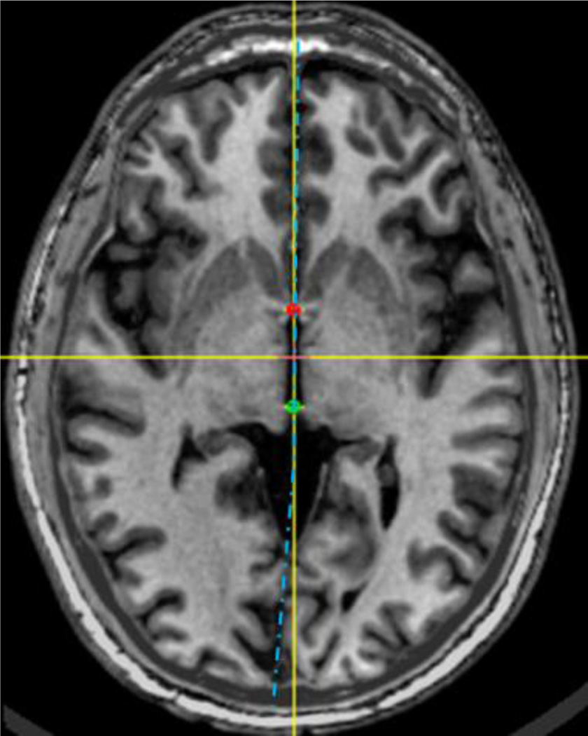
For the MSP, most existing methods can be categorized into two types: (i) methods maximizing a global symmetry score, (ii) methods detecting the IF. The first type of approaches assumes global bilateral symmetry and maximizes a similarity measure between the original brain scan and its reflected version [15]–[18]. However, there is no perfect bilateral symmetry in the human brain, not only for pathological cases but even for normal cases. As shown in Fig. 1 for a control subject, an effect known as brain torque occurs when the left occipital lobe or the right frontal lobe is larger than its counterpart in the other hemisphere [25]. Hence these methods may suffer from sensitivity to brain asymmetry and also often from high computational cost, while they may generalize well to other image modalities. On the other hand, approaches of the second type identify the IF from its intensity and textural features or by locally optimizing a symmetry measure, as local symmetry could be assumed in the vicinity of the IF region. The MSP is then determined by fitting a plane to those detected points or line segments [19]–[23]. These methods are generally more robust to abnormalities but more sensitive to outliers in the set of feature points. A robust outlier removal method is usually required to achieve the desired accuracy.

Fig. 1.

An example of the brain torque effect. The MSP represented as the vertical yellow axis deviates in the posterior region from the blue dotted curve which separates the hemispheres symmetrically on this slice.

Recently, learning-based methods using random forests have gained popularity for landmark and plane detection. Random forests are an ensemble supervised learning technique for classification or regression. In this approach a multitude of decision trees are constructed by evaluating a random subset of features at each node to split the data. The output of these trees is then aggregated to produce a final prediction [26]. In [27], Dabbah et al. used random forests as a classifier to localize anatomical landmarks in CT. Hough forests, which combine random forests with generalized Hough transform, are used to detect points to drive an active shape model on 2D radiographs [28], to find a rough position for the center of vertebrae in MR images [29], and most recently to localize the parasagittal plane in ultrasound images [30]. Schwing et al. [24] proposed to use adaptive random forests to jointly identify five distinct landmarks in the MSP in MR T1 images and estimate the plane via a least squares fit of these landmarks.

We have previously proposed a learning-based framework using regression forests to detect the AC and PC [31]. Here, we extend our previous work and augment it by also localizing the MSP. Since the AC, PC, and MSP have different local appearances from other points in the image, we hypothesize that a nonlinear regression can be used to estimate the relationship between the local appearance of a point and its probability to be the AC, the PC, or in the MSP. Compared to exiting techniques, our method is conceptually the most similar to the approach of Schwing et al. [24] in that a learning framework is used in both to detect the plane. We do, however, regress the distance from a point to the plane directly as opposed to its distance to selected landmarks as done in [24] because those landmarks may not be a perfect indicator of the plane due to the brain asymmetry.

The algorithm we propose is fast, accurate, and robust. It does not rely on any preprocessing of the images such as edge enhancement, nor does it require any segmentation or registration. Instead, we extract multi-scale contextual features for points in a set of training images and build random forests regression models to learn the probability for each sample to be the AC, the PC, or in the MSP. We employ three-stage coarse-to-fine models, with the first one operating on a down-sampled image to roughly localize the landmark or the plane and the second and third models to fine-tune the position. We evaluate our algorithm in a leave-one-out fashion using a large clinical dataset of 100 subjects. We also compare our method to state-of-the-art methods including an atlas-based approach with six well-established nonrigid registration algorithms and a publicly available implementation of a model-based approach for the AC and PC, as well as a publicly available implementation of a global symmetry-based approach for the MSP. We further test the sensitivity of our algorithm to anatomic abnormality, image quality, and parameter values.

II. Methods

A. Image Data

We select 100 subjects from a data repository we have created over a decade for DBS surgeries [32]. All images in our data set are T1-weighted sagittal MR volumes with approximately 256×256×170 voxels and 1mm in each direction, acquired with the SENSE parallel imaging technique (T1 W/3D/TFE) on a 3 Tesla Phillips scanner (TR = 7.92 ms, TE = 3.65 ms). These images have similar pose with small differences in head orientation and position, and also similar field of view (FOV), i.e., they cover the entire head. All images have been acquired as part of the normal delivery of care and every subject was consented to participate in this study.

For the AC and PC, two raters manually identified these points for each subject. These two raters followed the same protocol to select the AC and PC and were given sufficient time for accurate localization. The inter-rater variability is 0.57±0.47mm for the AC and 0.57±0.37 mm for the PC. Gold standard AC and PC are computed as an average of the selections by the two raters.

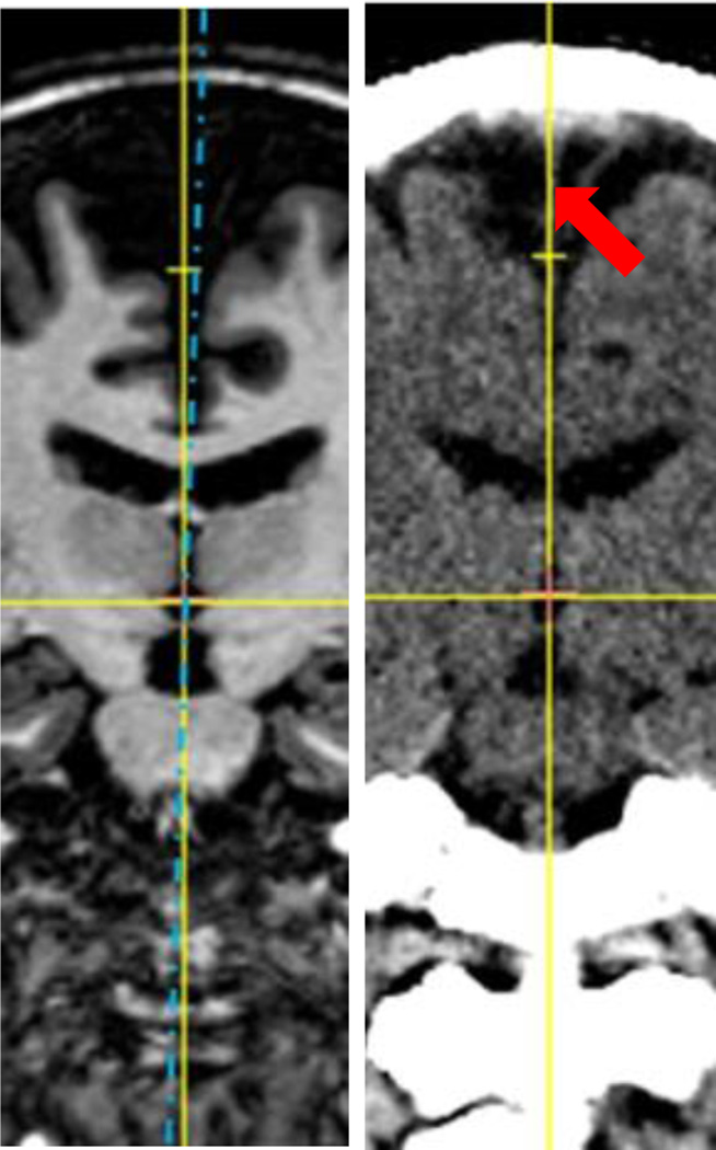
For the MSP, one rater manually selected the plane for each subject. Given the gold standard AC and PC, the MSP could be defined using any other point on the IF. However, cerebral atrophy that affects some DBS patients results in a widening of the IF. This makes the point selection on the IF ambiguous. In order to uniquely define the MSP, we follow the approach used clinically by an experienced neurosurgeon which relies on the falx cerebri, as illustrated in Fig. 2 and 3. The falx cerebri is a sickle-shaped fold of dura mater that descends vertically in the IF [33]. It is usually visible in CT but not in MR T1 images. Hence we used the CT volumes of the same patients and rigidly registered them to their corresponding T1 volumes. After the registration, the CT image and the gold standard AC and PC were loaded into a visualization software. A random point on the falx cerebri was selected first to establish an initial AC-PC coordinate system. The origin of this coordinate system is defined as the midpoint between the AC and the PC, with the x-axis perpendicular to the MSP pointing to the right, the y-axis pointing from the PC to the AC, and the z-axis pointing superiorly in the MSP. The CT image was then resampled in this coordinate system in which the xz planes correspond to the coronal slices. The MSP was then refined using coronal slices by varying the orientation of the plane to align it with the falx cerebri as accurately as possible. As the brain torque effect mostly causes the MSP to curve in the anterior and posterior regions of the brain, we used the midbrain region to define it, i.e., we used coronal slices that are anterior to the PC and posterior to the AC. After manual adjustment, the AC-PC coordinate system was updated and the CT image resampled in the new system for visual check in axial, coronal, and sagittal views. This process was repeated until the plane was visually deemed to be satisfactory.

Fig. 2.

Illustration of the MSP selection. The vertical yellow axis is the selection based on the falx cerebri, shown as the bright line on the right pointed by the red arrow, and the blue dotted line is one possible plane when selecting the MSP in MR T1 image.

Fig. 3.

A zoomed view of the CT slice in Fig. 2.

The gold standard AC and PC points together with the manual selection of the MSP are used as ground truth for the training and the evaluation of our learning-based method.

B. Problem Formulation

We use a voxel-level training solution based on regression forests to localize the landmarks and the plane. For each voxel, we extract a set of features that describe textural context variation at different scales, as proposed by Pauly et al. [34]. This is realized by applying a random displacement to a voxel x, calculating the mean intensities of a 3D cuboidal region $R_x^s$ centered on x and of a similar region $Q_x^{s,m}$ of the same size but centered on the displaced voxel, and subtracting these two:

$$f^m=\frac{1}{|R_x^s|}(\sum _{x\prime \in Q_x^{s,m}}I(x\prime )-\sum _{x\prime \in R_x^s}I(x\prime ))$$ (1)

where I is the intensity, and s is the current scale, i.e., a particular size of the cuboidal region. Four scales are used and they correspond to window sizes of 4, 8, 16, and 32. This process is repeated M = 2000 times to obtain the feature set ${\{f^m\}}_{m=1}^M$.

Each voxel is associated with a probability p to be the AC, the PC, or in the MSP that a model is trained to detect. This probability follows a truncated Gaussian distribution based on its Euclidean distance d to the ground truth AC, PC, or MSP:

$$p=\{\begin{array}{cc}{e}^{-\frac{d^2}{2{\sigma }^2}}\hfill & d>d_{th}\hfill \\ 0\hfill & d\le d_{th}\hfill \end{array}$$ (2)

where σ is the standard deviation of the Gaussian function. We truncate this function at p = 0.1 to speed up the training process.

Given a number of training pairs ${\{{\overrightarrow{f}}_n,p_n\}}_{n=1}^N$, random forests aim to learn a nonlinear mapping from the feature space {f⃗} to the probability space {p}. Hence the AC, PC, and MSP localization problem can now be formulated as first finding a set of voxels in the images that have a high probability to be the AC, PC, or in the MSP and then use these points to determine the landmarks or the plane.

C. Regression Forests

We use 20 regression trees to construct the forest. For each tree, a bootstrap of two thirds of the training samples is randomly selected and fed to the root node of the tree. Given the training samples ${\{\overrightarrow{f_n},p_n\}}_{n=1}^{N\prime }$ at a particular node, we seek to select a feature f^m and a threshold t to best split the data. The splitting criterion minimizes:

$$t,m=\underset{t,m}{\text{arg min}}MSE(\{p_n:f_n^m<t\})+MSE(\{p_n:f_n^m\ge t\}$$ (3)

where MSE is the mean squared error. A subset of 500 features is randomly selected to estimate the splitting threshold. A tree stops growing if the number of samples arriving at leaf nodes is smaller than 5 or if the best split threshold cannot be found.

Each leaf of the trees stores the mean probability of all samples arriving at that node to be a point of interest and this is used as a predictor. When a test sample comes, each tree contributes to a prediction. The mean and the variance of these predictions across trees are calculated and outputted for this test sample.

D. Training Phase

We train separate models for the AC, PC, and MSP. For each, we build three stage coarse-to-fine models, one on down-sampled by 4 images, one on down-sampled by 2 images, and one on full resolution images. This results in nine models to train for one training dataset.

Sampling strategy

Since all images in our dataset have similar pose and FOV, it is sufficient to search for the landmarks or the plane in a region of interest instead of searching the entire image. Thus, when training the model, for each image, we evaluate a set of points within a region of interest.

For the AC and PC, this region of interest is a cube centered on the ground truth points at each resolution level. It is a 15×15×15 voxel³ cube that covers a 60×60×60 mm³ volume at the coarsest level, a size that we have found large enough to account for the variations in the AC and PC positions across all images in the dataset. For each training subject, we use all the voxels in these cubes to generate the training samples.

For the MSP, at the coarse level, we follow the same strategy we use for the AC and PC to define a pseudo landmark in the MSP and define a cube centered on this point to be the region of interest. This point is selected to be on the z-axis, i.e., in the MSP plane, +50mm away from the origin in the AC-PC coordinate system established by the ground truth AC, PC, and MSP. We refer to this point as the mid-plane point (MP) and calculate the MP for each training subject. We use all the voxels in the 15×15×15 voxel³ cube centered on the MP as training samples as we have done for the AC and PC. For the next two resolution levels, as the MSP can already be roughly localized at the coarsest level, we only need to sample points that are spatially close to the MSP to further distinguish them from the true MSP. Hence we define the region of interest to be a rectangular cuboid encompassing the plane and aligned with the axes of the AC-PC coordinate system. At the down-sampled by 2 level, coordinates of the lower left corner and upper right corner are (−15mm, −15mm, −30mm) and (+15mm, +15mm, +90mm), respectively. At the full resolution level, we narrow the region of interest to [−7mm, +7mm] in the x, i.e., lateral direction, for further refinement. Voxels in the original image space are transformed into the AC-PC space first to check whether they fall into the region of interest, and those that satisfy this condition are considered as candidates. This leads to a large number of candidate points for training that cannot fit into the main memory. We address this issue by randomly sampling a fixed number of candidate points for each training subject.

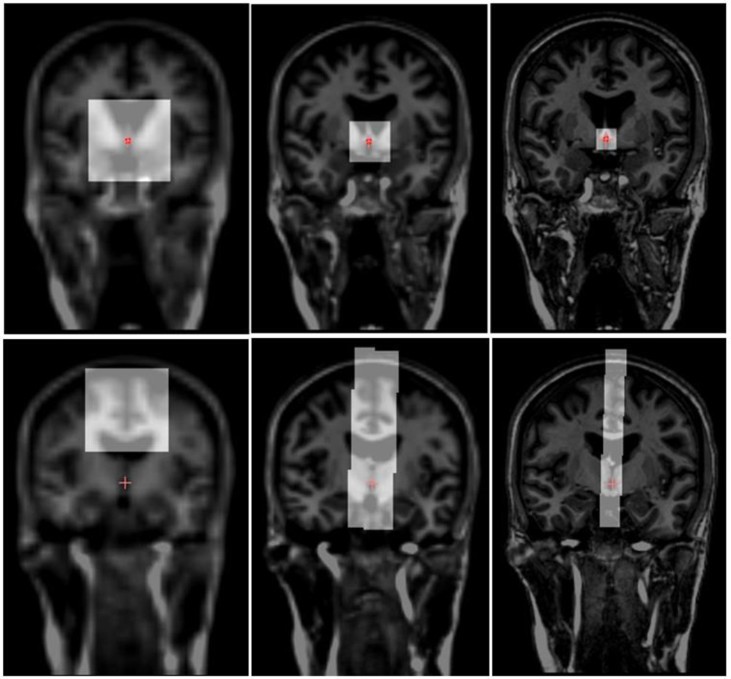
An example of the training regions from which samples are drawn at the different resolution levels is shown in Fig. 4, with the top row illustrating the AC regions and the bottom row illustrating the MSP regions.

Fig. 4.

Sampling regions for the AC (top row) and the MSP (bottom row) of a training subject at down-sampled by 4 (left), down-sampled by 2 (middle), and full resolution level (right), each overlaid on the corresponding image.

E. Testing Phase

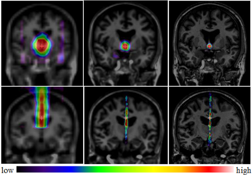
Given a test image, following the hierarchical approach described earlier, we first down-sample the image by 4 and start testing using the models built at this resolution level. At each level, we sequentially test for the AC, PC, and MSP. We initialize the search center from this model by averaging the ground truth AC, PC, and MP of all training subjects, and search within a 21×21×21 voxel³ window on a regular grid. A response map is generated for each landmark, displaying the mean probabilities p̄ of the voxels to be the trained landmark. For the AC and PC, the voxel associated with the highest probability is then used as the search center for the next level. For the MSP, a plane is estimated from the response map for the MP together with the AC and PC detected at this level, and this estimation is used to define the search region for the next level. We will explain in detail how to estimate the plane later. We continue this testing process for the next two resolution levels. For those two levels, the testing samples for the AC and PC are the points within a 21×21×21 voxel³ volume with its search center estimated from the previous level. For the MSP, the AC-PC coordinates of all voxels are first calculated based on the AC, PC, and MSP estimated from the previous level. The testing samples are those whose AC-PC coordinates are within [−15mm, +15mm] in the×direction, [−15mm, +15mm] in the y direction, and [−30mm, +90mm] in the z direction at the down-sampled by 2 level, and [−7mm, +7mm] in the × direction, [−15mm, +15mm] in the y direction, and [−30mm, 90mm] in the z direction at the full resolution level. An example of the response maps at different levels for one testing subject is illustrated in Fig. 5, with the top row illustrating the AC response maps and the bottom row illustrating the MSP response maps.

Fig. 5.

Response maps for the AC (top row) and the MSP (bottom row) of a testing subject at down-sampled by 4 (left), down-sampled by 2 (middle), and full resolution level (right), each overlaid on the corresponding image.

Mean-shift refinement for the AC/PC

When reaching the full resolution level, the final prediction for the AC and PC is made via weighted mean shift, a technique that is used to localize the maximum of a density function given discrete data sampled from that function [35]. Starting with an initial estimate x⁽⁰⁾, mean shift iteratively re-estimates the mean by weighting each point in its neighborhood, with the value of the weight determined by its distance to the current estimate and the probability of this point to be the trained landmark:

$$x^{(t+1)}=\frac{{\sum }_{{x_i}^{(t)}\in N(x^{(t)})}K({x_i}^{(t)}-x^{(t)})·\overline{{p_{\iota }}^{(t)}}·{x_i}^{(t)}}{{\sum }_{{x_i}^{(t)}\in N(x^{(t)})}K({x_i}^{(t)}-x^{(t)})·\overline{{p_{\iota }}^{(t)}}}$$ (4)

where x^(t) is the current estimate, x_i^(t) is a point in its neighborhood N(x^(t)), K(x_i^(t)−x^(t)) = e^{−k‖x_i(t)−x(t)‖2} is a Gaussian kernel, and $\overline{{p_{\iota }}^{(t)}}$ is the value of x_i^(t) in the response map which corresponds to the probability averaged across all trees.

We choose the initial estimate x⁽⁰⁾ to be the position of the testing sample with the maximum probability in the response map and iteratively update x^(t) until it converges. The output of this estimate is the final prediction for the AC/PC.

Weighted least squares fitting for the MSP

We represent the MSP as:

$$ax+by+cz+d=0,s.t.\Vert [a,b,c]\Vert =1$$ (5)

where a,b,c,d are the parameters that uniquely define the plane.

At each testing stage, we need to estimate the MSP using its response map along with the current AC and PC estimates. This is done by selecting a set of points that have a high probability p̄ to be in the MSP and fitting a plane to those points. To perform a robust linear regression, we compute a weighted least squares solution to account for the degree of uncertainty per point:

$$\underset{a,b,c,d}{\text{min}}\sum _{i=1}^{N\prime }{(a{x}_i+b{y}_i+c{z}_i+d)}^2·w_i,s.t.\Vert [a,b,c]\Vert =1$$ (6)

where N′ is the number of candidates, and w_i is the associated weight for sample (x_i, y_i, z_i).

For each candidate, we define its weight to be the square of the mean of the predictions divided by the variance of the predictions across all trees:

$$w_i={\overline{p_{\iota }}}^2/\mathit{\text{var}}(\overrightarrow{p_{\iota }})$$ (7)

Where $\overline{p_{\iota }}$ indicates how close this point is to the MSP as predicted by the model, and $\mathit{\text{var}}(\overrightarrow{p_{\iota }})$ indicates the model’s confidence about $\overline{p_{\iota }}$.

The final MSP prediction is thus the weighted least squares estimate at the full resolution level.

F. Comparison to Other Methods

For the AC and PC, we compare our results with those obtained by atlas-based registration, including affine only, and affine + nonrigid registration, a technique routinely used for automatic identification in DBS procedures [36]. We choose one atlas used by Pallavaram et al. [36] to be the reference and project its AC and PC points onto the 100 subjects through registration. An affine transformation is estimated first by an intensity-based technique that uses Mutual Information [37]–[38] as its similarity measure. The results are visually checked and manually corrected if a failure is observed. Then nonrigid registration is performed with a series of well-established algorithms, including the Adaptive Basis Algorithm (ABA), a variation of ABA that is tuned for deep brain structures referred to as the Adaptive Basis Algorithm with bounding box (LABA) [39], Diffeomorphic Demons (DD) [40], Symmetric Normalization (SyN) [41], Fast Free Form Deformation (F3D) [42], and Automatic Registration Toolbox (ART) [43]. A detailed description of those algorithms can be found in [44]. We also compare our method to a publicly available toolkit called YUKI which implements a recently proposed model-based approach to detect the AC and PC [12].

For the MSP, we compare our method to the same toolkit YUKI, which also implements a global symmetry-based approach to localize the plane [15].

III. Results

A. Leave-one-out Validation

We have conducted a leave-one-out validation, which uses 99 volumes for training and the last one for testing, and repeats this process 100 times.

Results for the AC and PC

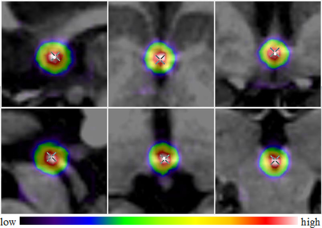
A representative example of response maps at the full resolution level is shown in Fig. 6, with the top row showing the AC response map and the bottom row showing the PC response map. The maps are overlaid on top of the original images, with the cross indicating the ground truth and the white dot our prediction. As shown in Fig. 6, the ground truth AC and PC have high probabilities and are close to our estimations (0.55mm differences for both AC and PC).

Fig. 6.

A representative example of response maps for AC (top row) and PC (bottom row) in sagittal (left), axial (middle), and coronal (right) views.

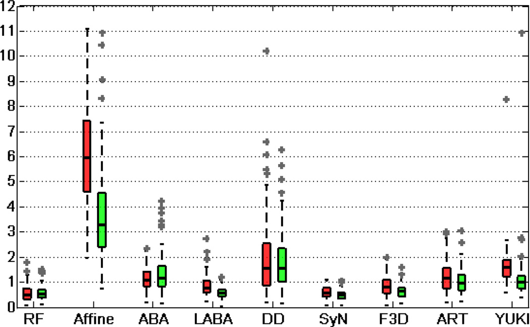
To quantitatively evaluate the accuracy of the algorithm, we use the 3D Euclidean distance between the automatically detected landmarks and the ground truth. We refer to our algorithm as RF (Random Forests) in the following text. Fig. 7 shows the boxplot of errors using different methods for the AC and PC. There are some outliers with errors beyond the maximum range of the y-axis (12mm), which are not shown in these figures. This includes 2 cases using Affine, 4 cases using YUKI for the AC, and 4 cases using YUKI for the PC. We also report error statistics for the AC in Table I and PC in Table II. We have excluded those above-mentioned outliers when computing mean, maximum, and standard deviations so as not to bias the comparisons. Table I and II demonstrate that our method leads to smaller mean, maximum, and standard deviation of errors for the AC and PC than the registration-based methods using Affine, ABA, DD, F3D, and ART, as well as the toolkit YUKI.

Fig. 7.

Boxplot of errors for the AC (red) and PC (green) in millimeters.

TABLE I.

STATISTICS OF ERRORS BETWEEN THE AUTOMATICALLY DETECTED AC USING DIFFERENT METHODS AND THE GROUND TRUTH AC POSITIONS

Error (ε): (mm) (AC)	Cases with ε<1	Cases with 1≤ ε<2	Cases with 2≤ ε<3	Cases with ε≥3	Mean	Max.	Std.
RF	95	5	0	0	0.55	1.78	0.30
Affine	0	1	2	97	5.96	11.06	1.87
ABA	43	53	4	0	1.12	2.35	0.48
LABA	73	25	2	0	0.83	2.73	0.40
DD	29	32	22	17	1.96	10.18	1.58
SyN	94	6	0	0	0.60	1.10	0.24
F3D	67	33	0	0	0.86	1.98	0.39
ART	40	52	8	0	1.19	2.99	0.60
YUKI	17	65	13	5	1.58	8.26	0.82

TABLE II.

STATISTICS OF ERRORS BETWEEN THE AUTOMATICALLY DETECTED PC USING DIFFERENT METHODS AND THE GROUND TRUTH PC POSITIONS

Error (ε): (mm) (PC)	Cases with ε<1	Cases with 1≤ ε<2	Cases with 2≤ ε<3	Cases with ε≥3	Mean	Max.	Std.
RF	93	7	0	0	0.56	1.50	0.28
Affine	1	13	28	58	3.68	10.90	1.88
ABA	38	51	5	6	1.33	4.23	0.75
LABA	93	7	0	0	0.57	1.18	0.23
DD	23	43	22	12	1.83	6.25	1.15
SyN	99	1	0	0	0.47	1.07	0.19
F3D	90	10	0	0	0.66	1.61	0.28
ART	54	43	2	1	1.02	3.04	0.49
YUKI	51	41	3	5	1.13	10.91	1.09

We also performed one-sided paired Wilcoxon signed-rank statistical tests to determine whether or not the medians of errors using our method are smaller than those using the other methods. The p values are shown in Table III. P values smaller than the significance level 0.05 are marked in red bold. These results show that our method is significantly better than most of the other methods. Indeed, it significantly reduces the AC and PC localization errors compared to the registration-based approaches using Affine, ABA, DD, F3D, and ART, as well as the publicly available toolkit YUKI.

TABLE III.

P VALUES OF WILCOXON TESTS BETWEEN THE ERRORS OF AC/PC DETECTED BY OUR METHOD AND ERRORS OF THOSE DETECTED BY OTHER AUTOMATIC METHODS

P	Affine	ABA	LABA	DD	SyN	F3D	ART	YUKI
AC	0.00	0.00	0.00	0.00	0.07	0.00	0.00	0.00
PC	0.00	0.00	0.23	0.00	1.00	0.00	0.00	0.00

Results for the MSP

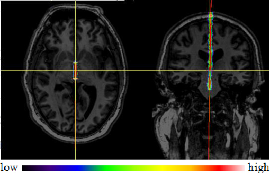
A representative example of response maps at the full resolution level is shown in Fig. 8 and 9, with the maps overlaid on top of the full resolution images resampled in the AC-PC coordinate system established by the ground truth AC, PC, and MSP. The vertical yellow axis represents the ground truth MSP and the red line represents the MSP detected by our algorithm. As shown in Fig. 8 and 9, points in the plane have high probabilities and our estimation is close to the manual selection (1.10° difference in the normal direction).

Fig. 8.

A representative example of response maps for the MSP in the axial (left) and coronal (right) views.

Fig. 9.

A zoomed view of the right panel in Fig. 8.

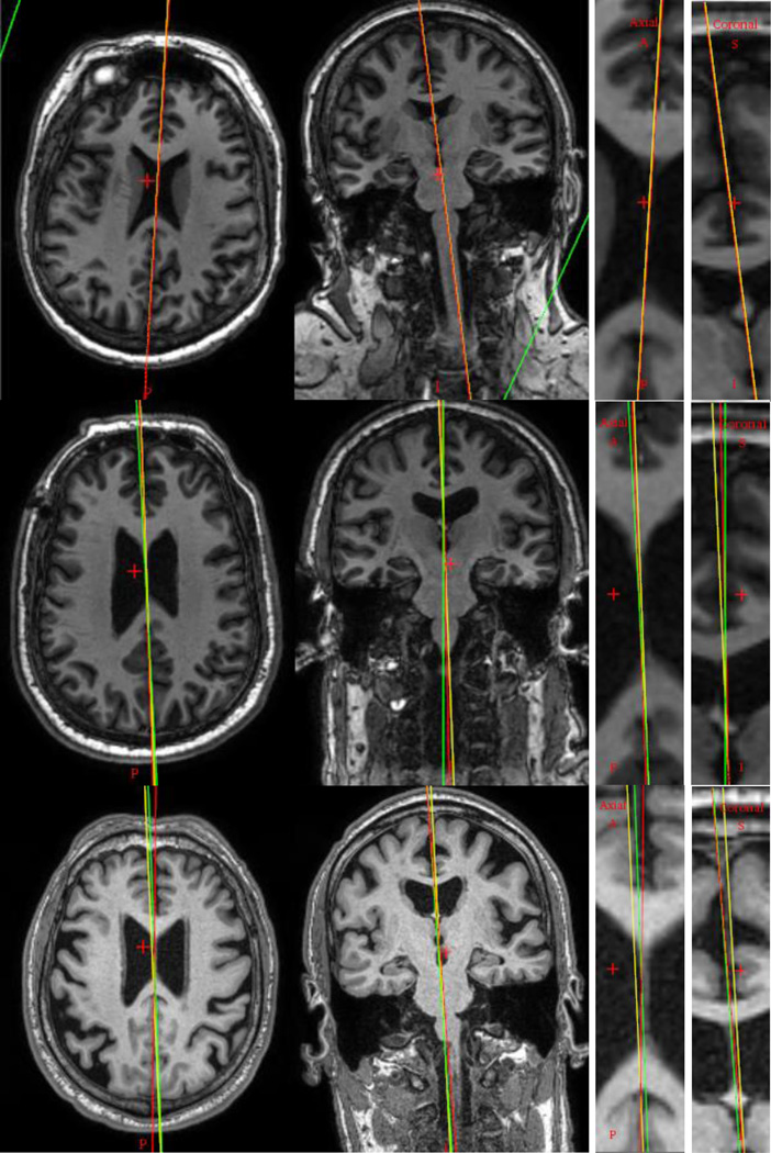
The best, an average, and the worse results are shown in Fig. 10 in the original image space. As before the red lines represent our estimations and the yellow lines the ground truth.

Fig. 10.

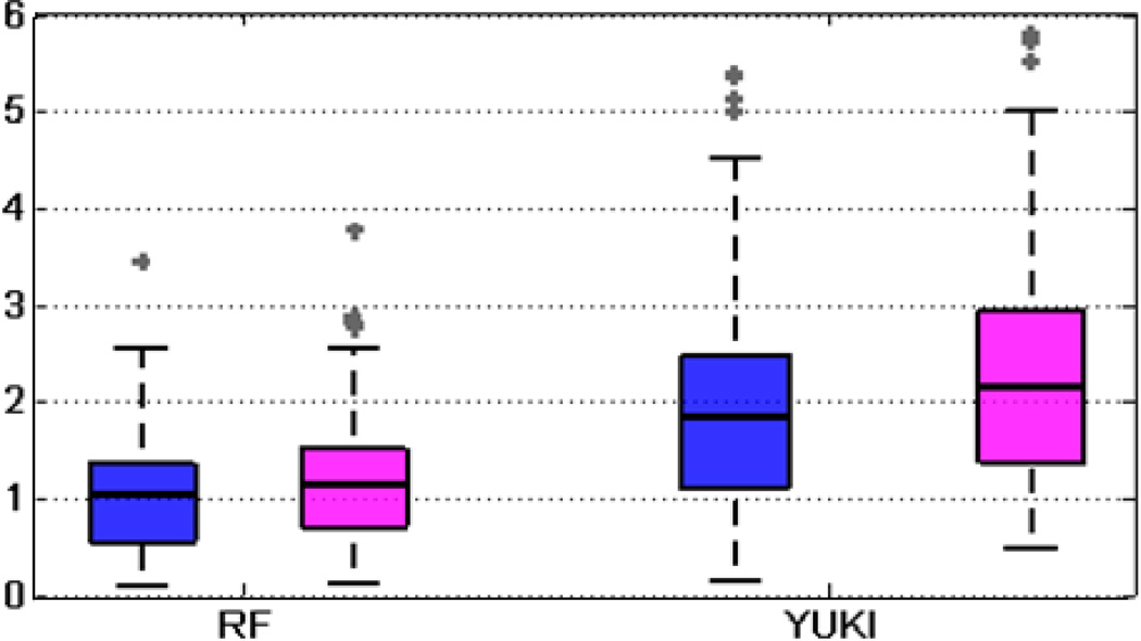
The best (top row), an average (middle row), and the worst (bottom row) MSP results using our proposed method. Ground truth MSPs are shown as yellow lines, our results as red lines, and the YUKI results as green lines.

To quantitatively evaluate the accuracy of our algorithm, we use the angular differences in the normal direction between the automatically detected MSP and the ground truth MSP as a measure of error. We also use a metric called average z-distance proposed by Ruppert et al. [18]. Referring to (6), this metric is computed as the absolute difference in the z coordinate in voxels between the ground truth plane and the estimated plane, averaged for all possible pairs of x and y values. This measure provides a sense of the average distance between the planes. Fig. 11 shows the boxplot of errors in the normal direction and in the average z-distance for our method and for YUKI. There are some outliers with errors beyond the maximum range of the y-axis (6° or 6 voxels), which are not shown in these figures. This includes 3 cases using YUKI. We also report error statistics for the normal direction in Table IV and for average z-distance in Table V. We have excluded those above-mentioned outliers for YUKI when computing mean, maximum, and standard deviations in order not to bias the comparisons. Table IV and V demonstrate that our method leads to smaller mean, maximum, and standard deviation of errors in the normal direction and in the average z-distance compared to the toolkit YUKI.

Fig. 11.

Boxplot of errors for the MSP in the normal direction in degrees (blue) and in average z-distance in voxels (magenta).

TABLE IV.

STATISTICS OF ERRORS IN THE NORMAL DIRECTION BETWEEN THE AUTOMATICALLY DETECTED MSP USING DIFFERENT METHODS AND THE GROUND TRUTH MSP

Error (ε): (°) (MSP)	Cases with ε<1	Cases with 1≤ ε<2	Cases with 2≤ ε<3	Cases with ε≥3	Mean	Max.	Std.
RF	49	39	11	1	1.08	3.43	0.66
YUKI	22	35	30	13	1.92	5.38	1.11

TABLE V.

STATISTICS OF ERRORS IN AVERAGE Z-DISTANCE BETWEEN THE AUTOMATICALLY DETECTED MSP USING DIFFERENT METHODS AND THE GROUND TRUTH MSP

Error (ε): (voxel) (MSP)	Cases with ε<1	Cases with 1≤ ε<2	Cases with 2≤ ε<3	Cases with ε≥3	Mean	Max.	Std.
RF	42	44	13	1	1.22	3.76	0.73
YUKI	13	30	33	24	2.25	6.12	1.20

We also performed one-sided paired Wilcoxon signed-rank statistical tests to determine whether or not the medians of errors using our method are smaller than those using YUKI. P values for both the angular errors and the average z-distance are smaller than the significance level 0.05, indicating that our method significantly outperforms YUKI.

B. Robustness Evaluation

We have conducted a series of experiments to assess the robustness of our method with regard to asymmetry of the brain, quality of the images, and rotational variations across subjects. Our experimental design is similar to those described by Liu et al. [16] and Hu et al. [23], except that we use clinical volumes instead of mirrored images. For each experiment, we randomly select 10 subjects from the dataset, generate simulated images under certain conditions, and localize target anatomies using the models previously trained for the unperturbed volume as described in section A. We measure the localization accuracy with the metrics used in section A, i.e., the distance error for AC and PC, the angular error and the distance error (average z-distance) for MSP. Results are averaged over the 10 subjects and shown in the following subsections.

Robustness with respect to brain asymmetry

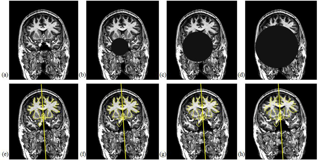
We simulate two different scenarios to introduce various pathologies that cause brain asymmetry. The first is to superimpose a spherical lesion with a specified position, radius, and intensity value in each test volume. The intensity value of the sphere replaces the value of the original voxels, as done in [23]. The second is to apply a local growth model with a specified seed point, radius, and growth rates to deform brain tissues. The growth model is a radially symmetric displacement field that produces deformations originating from the seed point and spreading gradually over the brain. The seed position is chosen to be away from the MSP to induce asymmetric deformation by the model. More details on this model can be found in [45]. For each test subject, we generate a set of simulated images with a range of radii for the sphere or the growth model as illustrated in Fig. 12 and localize the AC, PC, and MSP in those images.

Fig. 12.

Examples of simulated brain asymmetry for a test subject. Panel (a) shows one slice of the original image, and (e) is the same slice overlaid with the ground truth MSP and segmented structures represented as yellow contours. Panels (b)–(d) show the images superimposed with spherical lesions of radius 30mm, 50mm, and 70mm respectively, with all center points located at (XSize/2−20, YSize/2+20, ZSize/2−10) and intensity value=20. Panels (f)–(h) are the images deformed by growth models of radius 30mm, 50mm, 70mm respectively, with all seed points located at (XSize/2−20, YSize/2+20, ZSize/2−10).

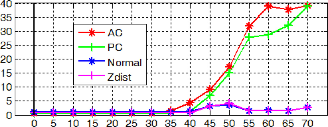
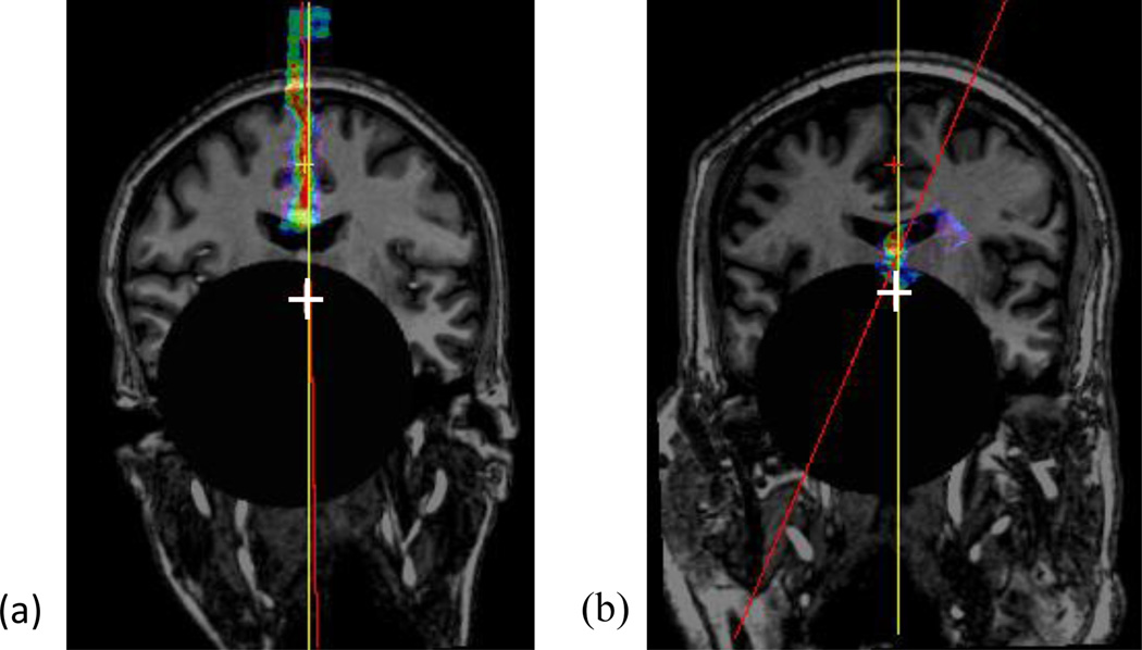
Fig. 13 shows the localization accuracy for the AC, PC, and MSP for different sizes of spherical lesions averaged over the 10 subjects. As shown in the figure, the AC and PC are localized well for spheres of small size; errors increase drastically when the radius is larger than 40mm. This is because the sphere has occluded the AC/PC region. In this situation, no valid AC/PC point exists in the image and detecting those points logically fails. Localization of the MSP is less sensitive to the size of the sphere, as illustrated by a successful case in Fig. 14 (a). An exception occurs for one subject when the radius is larger than 40mm, as shown in Fig. 14 (b). This is because we use the detected AC and PC to help define the search region for MSP, and the failure of AC/PC detection in this case leads to a highly skewed region with little coverage of the MSP. In practice, this scenario is unlikely to happen. If it does happen, our algorithm needs to be modified to handle failure cases for AC/PC so that these will not affect the MSP detection.

Fig. 13.

Localization errors for the AC, PC, and MSP in millimeters, degrees, or voxels with simulated spherical lesions of varying radius in millimeters.

Fig. 14.

A successful (a) and a failed (b) case for MSP detection with a spherical lesion of radius=50mm. Both images are resampled in the AC-PC reference system with their response maps for the MSP overlaid on top. The white cross indicates the ground truth AC and PC projected on this slice, the yellow line the ground truth MSP, and the red line the detected MSP.

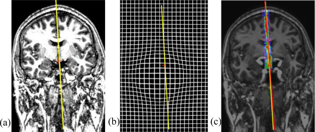
Fig. 15 shows the localization accuracy for the AC, PC, and MSP for different levels of tissue deformation averaged over the 10 subjects. As shown in this figure, the deformation we introduced only has a moderate impact on the results, with localization errors for the AC, PC, and MSP within 1.5 mm, degree, or voxel. The errors for MSP increase slightly with the amount of deformation. This is because the MSP deviates from planarity in those images; approximating it by a plane as we do in (5) is thus no more accurate. Fig. 16 illustrates such example for a test case, in which the effect of the tissue deformation is shown with a deformed grid (b) and an MSP detection result (c).

Fig. 15.

Localization errors for the AC, PC, and MSP in millimeters, degrees, or voxels with simulated tissue deformation using growth models of varying radius in millimeters.

Fig. 16.

A test case with a growth model of radius=50mm. Panel (a) is the original image, (b) is the grid deformed by the growth model, and (c) is the deformed volume overlaid with the response map for MSP, with the yellow line representing the ground truth MSP and the red line the detected MSP.

Robustness with respect to the noise level

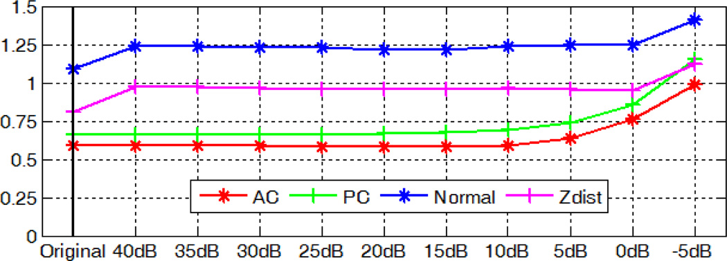
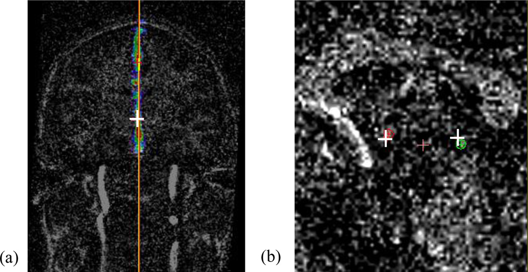
We artificially degrade each test volume by adding Gaussian white noise with zero mean and different variances. The localization accuracy of the AC, PC, and MSP for those degraded volumes averaged over 10 subjects at the same signal-to-noise ratio (SNR) level measured in decibel scale is shown in Fig. 17. As shown in the figure, our algorithm is able to detect AC and PC with mean error around 1mm and extract MSP with mean angular error within 1.5° and mean distance error within 1.5 voxel, even when the SNR is as low as −5dB. Results for a test case with SNR=−5dB are shown in Fig. 18, with 1.53mm error for AC, 1.82mm for PC, 1.06° angular error and 1.22 voxel distance error for MSP.

Fig. 17.

Localization errors for the AC, PC, and MSP in millimeters, degrees, or voxels with additive Gaussian noise of zero mean and varying variances.

Fig. 18.

Results for a degraded test volume with SNR=−5dB. Left panel (a) shows the image resampled in the AC-PC reference system with the response map for the MSP overlaid on top. The yellow line represents the ground truth MSP and red line the detected plane. Right panel (b) shows a zoomed sagittal view of the image, with the white cross being the projection of the ground truth AC/PC, and the red and green point the detected AC and PC respectively.

Robustness with respect to rotation

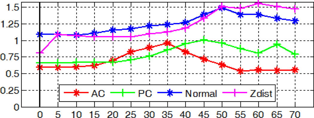
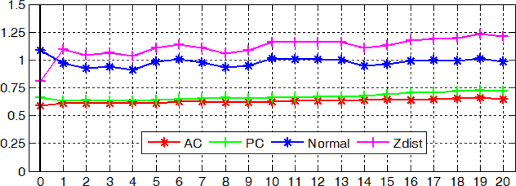
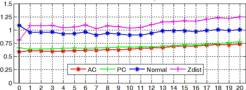
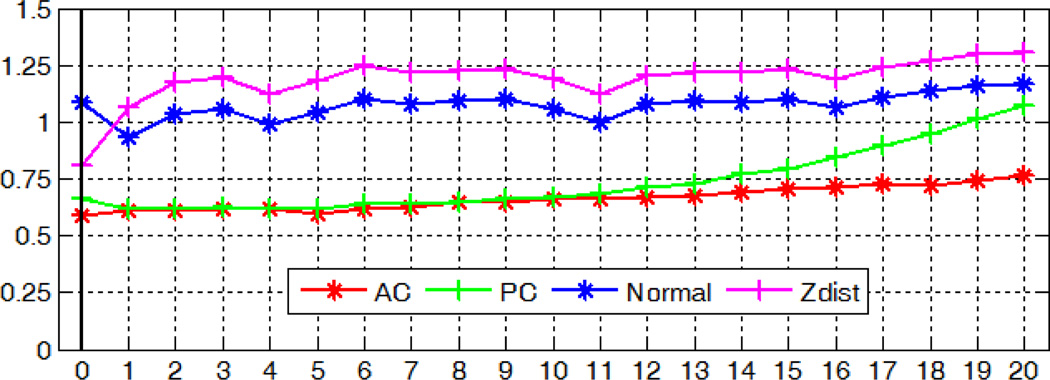
To study the sensitivity of our models to rotation, we rotate each test volume with respect to the center of the image around each of the x-, y-, and z-axis separately with angles varying from 0° to 20° in 1° intervals. For our images, the x-axis corresponds to the anterior-posterior direction, the y-axis the inferior-superior direction, and the z-axis the left-right direction.

Before running the tests, we slightly adjust our algorithm to handle rotations in test images. At each resolution level, we localize target anatomies as previously described, estimate the rotation angles around the x and y axes based on the current estimate of the MSP, and use these angles to re-orient the image for the next level. Localization errors for the AC, PC, and MSP are computed in the original space. Rotation correction is needed because of the limited rotational variations around the x and y axes in our dataset. During image acquisition, the scanner restricts the movement of the patient’s head from left to right or anterior to posterior. Patients can only freely move by looking up or down, which corresponds to rotation around the z-axis in our case. Rotation around the z-axis, however, does not affect the normal direction of the MSP. This leads to limited angular variations of MSP in our dataset. Models trained with those subjects do not generalize well with images with large rotations around x and y axes and the above modifications in the methodology are necessary.

With the modified method, the localization accuracy with regard to image rotations in the x-, y-, and z- axis is shown in Fig. 19, 20, and 21 respectively. Our algorithm for detecting the AC, PC and MSP is robust to rotations in all three directions, with mean errors up to 0.74mm for AC, 1.07mm for PC, 1.25° and 1.30 voxel for MSP.

Fig. 19.

Localization errors for the AC, PC, and MSP in millimeters, degrees, or voxels with simulated rotation around the x-axis from 0 to 20 degrees.

Fig. 20.

Localization errors for the AC, PC, and MSP in millimeters, degrees, or voxels with simulated rotation around the y-axis from 0 to 20 degrees.

Fig. 21.

Localization errors for the AC, PC, and MSP in millimeters, degrees, or voxels with simulated rotation around the z-axis from 0 to 20 degrees.

C. Parameter Sensitivity Analysis

We have also investigated the sensitivity of the parameters on the localization accuracy of the AC, PC and MSP. In this study, we select a subset of parameters that may critically affect the results. These parameters include (a) the number of trees in the forest, (b) the size of the node used to terminate the training process, i.e., the number of samples leaf nodes can contain, (c) the number of features to examine per node, and (d) the size of the Gaussian kernel in the mean shift algorithm. Among these parameters, (a)–(c) are used for model creation, i.e., training, and (d) for landmark detection. For each experiment, we test a set of parameter values with the 10 subjects used in section B.

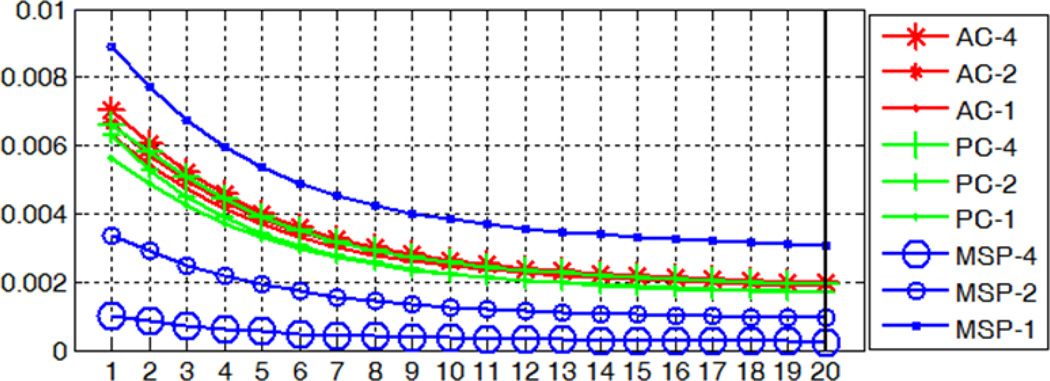
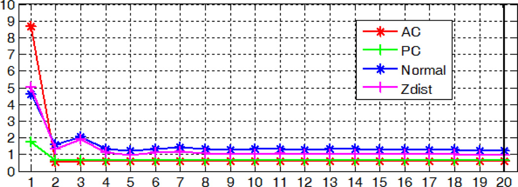
To test parameter (a), we plot the out-of-bag (OOB) error rate versus the number of trees for the nine models averaged over the 10 subjects in Fig. 22. The OOB error is estimated by feeding each tree with the training data left out in the construction of this tree as testing data and calculating the mean square difference between the true probabilities and the predictions. This has been shown to be an unbiased estimate of the test set error [26]. We downscaled the OOB errors for MSP by a factor of 10 for visualization purpose. As more trees are added, the OOB error first rapidly decreases and gradually reaches a plateau with 20, which is the number of trees we have used in section A.

Fig. 22.

OOB errors versus the number of trees for models built for the AC, PC, and MSP at three different resolution levels. Errors for MSP are downscaled by a factor of 10 for display purpose.

For parameter (a), we also assess its direct impact on the localization accuracy by detecting the AC, PC, and MSP with only a subset of trees to make predictions. Localization errors are shown in Fig. 23. Compared to Fig. 22, we observe the same trend that introducing more trees help reduce the errors, with a difference that few trees are actually needed. This is because while the OOB plot treats each sample equally, the localization task does not. Samples with low probabilities to be the landmark or in the plane have less effect on the localization accuracy if their errors are within the tolerance level, as those samples would be disregarded from voting for the final prediction.

Fig. 23.

Localization errors for the AC, PC, and MSP using models with different number of trees.

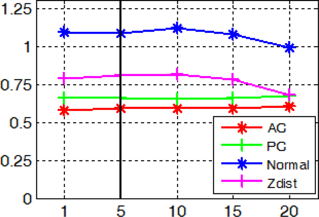
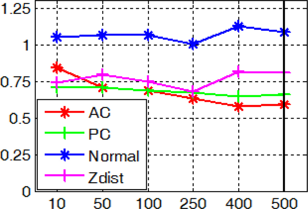
To test parameters (b) and (c), for each of the 10 subjects, we re-trained models as described in section A with the same training data but different parameter values. We vary parameter (b) in the interval [1, 20] with a step size of 5. A node size of 1 corresponds to fully grown trees. As the node size increases, the degree of pruning increases. For parameter (c), we test standard values as suggested in [26], i.e., $\sqrt{M}$ and log₂ M with M being the number of features for a sample. In our case, these correspond to ~10 and ~50 respectively. We also test a range of values between these and the one we have used in our experiments. We then localize the AC, PC, and MSP using those re-trained models. Sensitivity of the localization errors to parameters (b) and (c) is shown in Fig. 24 and 25 respectively. The values we have used in section A are shown with bold lines. These figures suggest that the size of the node and the number of features examined per node have little impact on the accuracy of our algorithm. While different parameter values may yield slightly better results than those we have used, for example, examining 250 features per node leads to smaller errors for MSP, the differences are marginal, i.e., within 0.1 degree or voxel.

Fig. 24.

Localization errors for the AC, PC, and MSP using models built with different size of the node to terminate training process.

Fig. 25.

Localization errors for the AC, PC, and MSP using models built with different number of features to examine per node.

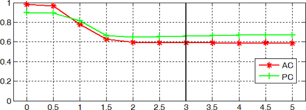
Fig. 26 shows the localization errors for the AC and PC when we vary parameter (d). Using a kernel with zero variance corresponds to identifying landmarks as the voxel with the highest probability, as done in [31]. When the variance of the Gaussian kernel increases, errors decline at first and then stabilize when the variance reaches 2. This indicates that the spatial smoothing of the response maps using the mean shift technique improves the AC/PC detection accuracy but the value of the variance has little effect when it is above 2.

Fig. 26.

Localization errors for the AC and PC in millimeters using Gaussian kernels with zero mean and varying variances.

IV. Discussion and Conclusion

In this paper, we propose a learning-based method to automatically detect the AC, PC, and MSP in MR T1 brain scans using random regression forests. We use 20 trees to construct the forest, a number we chose based on the plot of the OOB error versus the number of trees. We have performed a parameter sensitivity analysis, and results indicate that the size of the node used to terminate the training process and the number of features that are examined per node have little impact on the localization accuracy. The features we have used for learning are contextual features generated by randomly displacing vectors. In principle, the number of features could be indefinitely large. To keep the computation practical, only a random set of 2000 features are used. Recent work by Yaqub et al. [46] has suggested that with feature selection the performance of random forests could be enhanced for brain segmentation task in T1 images, one direction we would like to pursue in our work in the future.

We localize the landmarks and the plane using a semi-local search in the sense that the search is limited to a large region of interest. This is reasonable because all the images in our dataset have similar pose and FOV. If heterogeneous datasets with various orientations, dimensions, and field-of-views are involved, one will need to reorient the image first as we have done when evaluating the sensitivity of our method to rotation to be consistent with the training images or increase the size of the region of interest for training and testing at the coarse level. Our technique is developed on MR T1 images. However, extension to other image modalities is straightforward by building models for that particular image set.

We have conducted leave-one-out experiments to validate our method. Results have shown that our approach is accurate and robust, with 0.55±0.30mm and a maximum of 1.78mm error for the AC, 0.56±0.28mm and a maximum of 1.50mm error for the PC, a 1.08°±0.66° and a maximum of 3.43° angular error in the normal direction, as well as 1.22±0.73 and a maximum of 3.73 voxel of distance error in average z-distance for the MSP.

For the AC and the PC, we have compared our approach to single-atlas-based methods using six well-established nonrigid registration algorithms and also with a model-based approach that has been proposed recently and implemented in the publicly available toolkit YUKI. We have found that our algorithm outperforms four nonrigid registration methods (ABA, DD, F3D, and ART) as well as the toolkit YUKI in terms of accuracy and robustness; the improvements are statistically significant. Other registration methods (LABA and SyN) achieve similar or slightly better accuracy than ours. However, they rely on good affine initialization. In this study we have manually corrected 9 out of the 100 affine registrations so as not to bias the nonrigid registration results. In an automatic system such uncorrected affine registration may deteriorate the performance of nonrigid registrations and cause a failure in the AC and PC localization.

For the MSP, we have evaluated our method against a global symmetry-based approach implemented in the toolkit YUKI as well. Our results for both plane normal errors and average z-distances are statistically significantly better than those using YUKI. A thorough comparison to other state-of-the-art methods is nontrivial without any publicly available implementations and is out of the scope of this paper. However, a review of the literature shows that our method compares favorably to existing techniques. Indeed, in [18], Ruppert et al. compared their method to Volkau et al. [20], Teverovskiy et al. [17], and Bergo et al. [21] using average z-distance with 20 normal MR T1 images, and the results were 1.27±0.59, 1.84±1.14, 1.46±0.81, 1.46±0.93 voxel respectively. With a much larger clinical dataset of DBS patients, we achieved results (1.22±0.73) that are highly comparable to the best in [18] (1.27±0.59). In a most recent study which also employed a learning-based schema as discussed earlier [24], Schwing et al. reported angular errors in the normal direction of 1.08°±0.76°. This is the same mean as ours but their standard deviation is larger.

We have designed a set of experiments to test the robustness of our algorithm against asymmetry of the brain, poor image quality, and variation in rotations across subjects. Results show that our algorithm is tolerant to brain asymmetries such as spherical lesions and tissue deformations without occlusions of the AC/PC. It is also tolerant to high level of imaging noise and, with the modifications described in section III-B, to rotations for the AC, PC, and MSP in any direction.

Another advantage of our approach is the speed. Although registration methods such as SyN may be marginally more accurate, they generally take at least minutes, if not hours, to run. Our method is fast, taking only about 25 seconds on a standard desktop PC with 4 CPU cores and 8GB RAM to compute the AC, PC, and MSP all at once. The algorithm is implemented in C++ with parallelization. The computations for model training are done on the Advanced Center for Computing and Research Education (ACCRE) Linux cluster at Vanderbilt University.

We should note that as a supervised learning technique, our method generalizes the information learned from training data to the test data. To achieve the desired accuracy for a test case, patches extracted from this image should look somewhat similar to those in the training set. Fundamentally the performance of our algorithm is limited by the training data we use to build the models. For example, without modifications of our method, the lack of variations in rotation around the anterior-posterior and superior-inferior axes would lead to poor detection of the MSP on test cases with large rotations in those directions. Our algorithm could not manage occlusions of the AC/PC region either, as no such sample appeared in the training data. In order for the model to capture this information, the training set needs to be enriched to handle images with such variations.

There may be some bias towards our method when compared to YUKI, which can be freely downloaded [47]. First, YUKI was not trained on the same images we have used. In addition, it may have used a slightly different definition of the AC, PC, or MSP. For example, the AC could be marked by its center or its posterior edge; the MSP could be defined in other ways than using the falx cerebri. Those factors may account for some of the performance differences between YUKI and our method. To address this issue and permit a thorough comparison between algorithms, it would be beneficial to develop publicly available annotated datasets on which algorithms could be applied.

Biographies

Yuan Liu (S’10) received the B.Eng. degree in computer science from Northwestern Polytechnical University, Xi’an, China, in 2010. She is currently working toward the Ph.D. degree at the Department of Electrical Engineering and Computer Science, Vanderbilt University, Nashville, TN.

Her research interests include medical image processing, image-guided surgery, machine learning, and big data analytics.

Benoit M. Dawant (M’88–SM’03–F’10) received the M.S.E.E. degree from the University of Louvain, Leuven, Belgium, in 1983, and the Ph.D. degree from the University of Houston, Houston, TX, in 1988.

Since 1988, he has been with the Faculty of the Electrical Engineering and Computer Science Department, Vanderbilt University, Nashville, TN, where he is currently a Cornelius Vanderbilt Professor of Engineering. His main research interests include image-guided surgery and medical image processing, segmentation, and registration.

Current domains of application include the development of algorithms and systems to assist in the placement and programming of deep brain stimulators used for the treatment of Parkinson’s disease and other movement disorders, the placement and programming of cochlear implants used to treat hearing disorders, or the creation of radiation therapy plans for the treatment of cancer.

References

- 1.Schaltenbrand G, Wahren W. Guide to the Atlas for Stereotaxy of the Human Brain. Stuttgart, Germany: Thieme; 1977. [Google Scholar]
- 2.Talairach J, Tournoux P. Co-planar Stereotaxic Atlas of the Human Brain. Stuttgart, Germany: Thieme; 1988. [Google Scholar]
- 3.Starr PA. Placement of deep brain stimulators into the subthalamic nucleus or globus pallidus internus: technical approach. Stereotact. Funct. Neurosurg. 2003 Jul.79(3–4):118–145. doi: 10.1159/000070828. [DOI] [PubMed] [Google Scholar]
- 4.Nowinski WL, Thirunavuukarasuu A. Atlas-assisted localization analysis of functional images. Med. Image Anal. 2001 Sep.5(3):207–220. doi: 10.1016/s1361-8415(01)00043-3. [DOI] [PubMed] [Google Scholar]
- 5.Collins DL, Neelin P, Peters TM, Evans AC. Automatic 3D intersubject registration of MR volumetric data in standardized Talairach space. J. Comput. Assist. Tomo. 1994 Mar-Apr;18(2):192–205. [PubMed] [Google Scholar]
- 6.Han Y, Park H. Automatic brain MR image registration based on Talairach reference system. Proc. ICIP. 2003:1097–1100. doi: 10.1002/jmri.20168. [DOI] [PubMed] [Google Scholar]
- 7.Joshi S, Lorenzen P, Gerig G, Bullitt E. Structural and radiometric asymmetry in brain images. Med. Image Anal. 2003 Jun.7(2):155–170. doi: 10.1016/s1361-8415(03)00002-1. [DOI] [PubMed] [Google Scholar]
- 8.Pallavaram S, Yu H, Spooner J, D’Haese PF, Bodenheimer B, Konrad PE, Dawant BM. Intersurgeon variability in the selection of anterior and posterior commissures and its potential effects on target localization. Stereotact. Funct. Neurosurg. 2008 Mar.86(2):113–119. doi: 10.1159/000116215. [DOI] [PMC free article] [PubMed] [Google Scholar]
- 9.Verard L, Allain P, Travere JM, Baron JC, Bloyet D. Fully automatic identification of AC and PC landmarks on brain MRI using scene analysis. IEEE Trans. Med. Imag. 1997 Oct.16(5):610–616. doi: 10.1109/42.640751. [DOI] [PubMed] [Google Scholar]
- 10.Bhanu Prakash KN, Hu Q, Aziz A, Nowinski WL. Rapid and automatic localization of the anterior and posterior commissure point landmarks in MR volumetric neuroimages. Academic Radiol. 2006 Jan.13(1):36–54. doi: 10.1016/j.acra.2005.08.023. [DOI] [PubMed] [Google Scholar]
- 11.Zhang G, Fu Y, Wang S, Gao W. Automatic localization of AC and PC landmarks in T2-weighted MR volumetric neuroimages. Proc. ICIA. 2010:1830–1834. [Google Scholar]
- 12.Ardekani BA, Bachman AH. Model-based automatic detection of the anterior and posterior commissures on MRI scans. Neuroimage. 2009 Jul.46(3):677–682. doi: 10.1016/j.neuroimage.2009.02.030. [DOI] [PMC free article] [PubMed] [Google Scholar]
- 13.Pallavaram S, Yu H, D’Haese PF, Spooner J, Koyama T, Bodenheimer B, Kao C, Konrad PE, Dawant BM. Automated selection of anterior and posterior commissures based on a deformable atlas and its evaluation based on manual selections by neurosurgeons. Proc. SPIE Med. Imaging. 2007:65091C–65091C. [Google Scholar]
- 14.Anbazhagan P, Carass A, Bazin PL, Prince JL. Automatic estimation of midsagittal plane and AC-PC alignment on nonrigid registration. Proc. ISBI. 2006:828–831. [Google Scholar]
- 15.Ardekani BA, Kershaw J, Braun M, Kanno I. Automatic detection of the mid-sagittal plane in 3-d brain images. IEEE Trans. Med. Imag. 1997 Dec.16(6):947–952. doi: 10.1109/42.650892. [DOI] [PubMed] [Google Scholar]
- 16.Liu Y, Collins RT, Rothfus WE. Robust midsagittal plane extraction from normal and pathological 3-D neuroradiology image. IEEE Trans. Med. Imag. 2001 Mar.20(3):173–192. doi: 10.1109/42.918469. [DOI] [PubMed] [Google Scholar]
- 17.Teverovskiy L, Liu Y. Truly 3D midsagittal plane extraction for robust neuroimage registration. Proc. ISBI. 2006:860–863. [Google Scholar]
- 18.Ruppert GCS, Teverovskiy L, Yu CP, Falcao AX, Liu Y. A new symmetry-based method for mid-sagittal plane extraction in neuroimages. Proc. ISBI. 2011:285–288. [Google Scholar]
- 19.Brummer ME. Hough transform detection of the longitudinal fissure in tomographic head images. IEEE Trans. Med. Imag. 1991 Mar.10(1):74–81. doi: 10.1109/42.75613. [DOI] [PubMed] [Google Scholar]
- 20.Volkau I, Prakash KB, Ananthasubramaniam A, Aziz A, Nowinski WL. Extraction of the midsagittal plane from morphological neuroimages using the kullback-leibler’s measure. Med. Image Anal. 2006 Dec.10(6):863–874. doi: 10.1016/j.media.2006.07.005. [DOI] [PubMed] [Google Scholar]
- 21.Bergo FPG, Ruppert GCS, Falcao AX. Fast and robust mid-sagittal plane location in 3D MR images of the brain. Proc. BIOSIGNALS. 2008:92–99. [Google Scholar]
- 22.Wu H, Wang D, Shi L, Wen Z, Ming Z. Midsagittal plane extraction from brain images based on 3D SIFT. Phys. Med. Biol. 2014 Feb.59(6):1367–1387. doi: 10.1088/0031-9155/59/6/1367. [DOI] [PubMed] [Google Scholar]
- 23.Hu Q, Nowinski WL. A rapid algorithm for robust and automatic extraction of the midsagittal plane of the human cerebrum from neuroimages based on local symmetry and outlier removal. Neuroimage. 2003 Dec.20(4):2153–2165. doi: 10.1016/j.neuroimage.2003.08.009. [DOI] [PubMed] [Google Scholar]
- 24.Schwing A, Zheng Y. Reliable extraction of the mid-sagittal plane in 3d brain mri via hierarchical landmark detection. Proc. ISBI. 2014:1–4. [Google Scholar]
- 25.Toga AW, Thompson PM. Mapping brain asymmetry. Nat. Rev. Neurosci. 2003 Jan.4(1):37–48. doi: 10.1038/nrn1009. [DOI] [PubMed] [Google Scholar]
- 26.Breiman L. Random forests. Mach. Learn. 2001 Oct.45(1):5–32. [Google Scholar]
- 27.Dabbah MA. Detection and location of 127 anatomical landmarks in diverse CT datasets. Proc. SPIE Med. Imaging. 2014:903415–903415. [Google Scholar]
- 28.Lindner C, Thiagarajah S, Wilkinson JM, Consortium TA, Wallis GA, Cootes TF. Fully Automatic Segmentation of the Proximal Femur Using Random Forest Regression Voting. IEEE Trans. Med. Imag. 2013 Aug.32(8):181–189. doi: 10.1109/TMI.2013.2258030. [DOI] [PubMed] [Google Scholar]
- 29.Glocker B, Feulner J, Criminisi A, Haynor DR, Konukoglu E. Automatic localization and identification of vertebrae in arbitrary field-of-view CT scans. Proc. MICCAI. 2012:590–598. doi: 10.1007/978-3-642-33454-2_73. [DOI] [PubMed] [Google Scholar]
- 30.Yaqub M, Kopuri A, Rueda S, Sullivan PB, McCormick K, Noble JA. A Constrained Regression Forests Solution to 3D Fetal Ultrasound Plane Localization for Longitudinal Analysis of Brain Growth and Maturation. Proc. MLMI. 2014:109–116. [Google Scholar]
- 31.Liu Y, Dawant BM. Automatic Detection of the Anterior and Posterior Commissures on MRI Scans Using Regression Forests. Proc. EMBC. 2014:1505–1508. doi: 10.1109/EMBC.2014.6943887. [DOI] [PMC free article] [PubMed] [Google Scholar]
- 32.D’Haese PF, Pallavaram S, Li R, Remple MS, Kao C, Neimat JS, Konrad PE, Dawant BM. CranialVault and its CRAVE tools: A clinical computer assistance system for deep brain stimulation (DBS) therapy. Med. Image Anal. 2012 Apr.16(3):744–753. doi: 10.1016/j.media.2010.07.009. [DOI] [PMC free article] [PubMed] [Google Scholar]
- 33.Baehr M, Frotscher M. Duus' topical diagnosis in neurology: anatomy, physiology, signs, symptoms. 5th ed. Stuttgart, Germany: Thieme; 2012. [Google Scholar]
- 34.Pauly O, Glocker B, Criminisi A, Mateus D, Moller AM, Nekolla S, Navab N. Fast multiple organ detection and localization in whole-body MR Dixon sequences. Proc. MICCAI. 2011:239–247. doi: 10.1007/978-3-642-23626-6_30. [DOI] [PubMed] [Google Scholar]
- 35.Cheng Y. Mean shift, mode seeking, and clustering. IEEE Trans. Pattern Anal. Mach. Intell. 1995 Aug.17(8):790–799. [Google Scholar]
- 36.Pallavaram S, Dawant BM, Koyama T, Yu H, Neimat J, Konrad PE, D’Haese PF. Validation of a fully automatic method for the routine selection of the anterior and posterior commissures in magnetic resonance images. Stereotact. Funct. Neurosurg. 2009 Jun.87(3):148–154. doi: 10.1159/000209295. [DOI] [PMC free article] [PubMed] [Google Scholar]
- 37.Maes F, Collignon FA, Vandermeulen D, Marchal G, Suetens P. Multimodality image registration by maximization of mutual information. IEEE Trans. Med. Imag. 1997 Apr.16(2):187–198. doi: 10.1109/42.563664. [DOI] [PubMed] [Google Scholar]
- 38.Viola P, Wells WM., III Alignment by maximization of mutual information. Int. J. Comput. Vision. 1997 Sep.24(2):137–154. [Google Scholar]
- 39.Rohde GK, Aldroubi A, Dawant BM. The adaptive bases algorithm for intensity-based nonrigid image registration. IEEE Trans. Med. Imag. 2003 Nov.22(11):1470–1479. doi: 10.1109/TMI.2003.819299. [DOI] [PubMed] [Google Scholar]
- 40.Vercauteren T, Pennec X, Perchant A, Ayache N. Diffeomorphic demons: efficient non-parametric image registration. NeuroImage. 2009 Mar.45(1):S61–S72. doi: 10.1016/j.neuroimage.2008.10.040. [DOI] [PubMed] [Google Scholar]
- 41.Avants BB, Epstein CL, Grossman M, Gee JC. Symmetric diffeomorphic image registration with cross-correlation: evaluating automated labeling of elderly and neurodegenerative brain. Med. Image Anal. 2008 Feb.12(1):26–41. doi: 10.1016/j.media.2007.06.004. [DOI] [PMC free article] [PubMed] [Google Scholar]
- 42.Modat M, Ridgway GR, Taylor ZA, Lehmann M, Barnes J, Hawkes DJ, Fox NC, Ourselin S. Fast free-form deformation using graphics processing units. Comput. Meth. Prog. Bio. 2010 Jun.98(3):278–284. doi: 10.1016/j.cmpb.2009.09.002. [DOI] [PubMed] [Google Scholar]
- 43.Ardekani BA, Guckemus S, Bachman A, Hoptman MJ, Wojtaszek M, Nierenberg J. Quantitative comparison of algorithms for inter-subject registration of 3D volumetric brain MRI scans. J. Neurosci. Meth. 2005 Mar.142(1):67–76. doi: 10.1016/j.jneumeth.2004.07.014. [DOI] [PubMed] [Google Scholar]
- 44.Liu Y, H’aese PF, Dawant BM. Effects of deformable registration algorithms on the creation of statistical maps for preoperative targeting in deep brain -stimulation procedures. Proc. SPIE Med. Imaging. 2014:90362B–90362B. [Google Scholar]
- 45.Han Z. Ph.D. dissertation. Vanderbilt Univ., TN: EECS Dept.; 2011. Effect of non-rigid registration algorithms on the analysis of brain MR images with deformation based morphometry. [Google Scholar]
- 46.Yaqub M, Javaid M, Cooper C, Noble A. Investigation of the role of feature selection and weighted voting in random forests for 3D volumetric segmentation. IEEE Trans. Med. Imag. 2014 Feb.33(2):258–271. doi: 10.1109/TMI.2013.2284025. [DOI] [PubMed] [Google Scholar]
- 47. http://www.nitrc.org/frs/?group_id=90. [Google Scholar]