Measuring Asymmetric Interactions in Resting State Brain Networks

Abstract

Directed graph representations of brain networks are increasingly being used in brain image analysis to indicate the direction and level of influence among brain regions. Most of the existing techniques for directed graph representations are based on time series analysis and the concept of causality, and use time lag information in the brain signals. These time lag-based techniques can be inadequate for functional magnetic resonance imaging (fMRI) signal analysis due to the limited time resolution of fMRI as well as the low frequency hemodynamic response. The aim of this paper is to present a novel measure of necessity that uses asymmetry in the joint distribution of brain activations to infer the direction and level of interaction among brain regions. We present a mathematical formula for computing necessity and extend this measure to partial necessity, which can potentially distinguish between direct and indirect interactions. These measures do not depend on time lag for directed modeling of brain interactions and therefore are more suitable for fMRI signal analysis. The necessity measures were used to analyze resting state fMRI data to determine the presence of hierarchy and asymmetry of brain interactions during resting state. We performed ROI-wise analysis using the proposed necessity measures to study the default mode network. The empirical joint distribution of the fMRI signals was determined using kernel density estimation, and was used for computation of the necessity and partial necessity measures. The significance of these measures was determined using a one-sided Wilcoxon rank-sum test. Our results are consistent with the hypothesis that the posterior cingulate cortex plays a central role in the default mode network.

1 Introduction

Brain networks are primarily described in terms of functional connectivity and effective connectivity. Functional connectivity is defined as the temporal correlation between spatially remote neurophysiological events and effective connectivity is defined as the influence one neuronal system exerts over another [4]. Functional connectivity refers only to an undirected relationship between two distinct brain regions. Effective connectivity, on the other hand, can be used to describe the brain network as a directed graph. Two popular model-driven approaches for measuring effective connectivity from fMRI data are structural equation modeling (SEM) [11] and dynamic causal modeling (DCM) [5]. In SEM, the covariances of activity between brain regions are used to calculate path coefficients representing the magnitudes of influences corresponding to directional paths. On the other hand, DCM models the brain as a nonlinear dynamic system in which external stimuli produce changes in brain activity. Responses to the stimuli are measured and used to estimate model parameters representing the effective connectivity between brain regions. Recently, DCM has been extended to resting state fMRI data [6]. Note that DCM models interactions at the neuronal rather than the hemodynamic level. Since changes in effective connectivity occur at a neuronal level, DCM is frequently the preferred method for making inferences about effective connectivity from fMRI data. However, a limitation of DCM is that it requires a priori knowledge and the estimation of a large number of parameters, which can be difficult in the context of resting state fMRI data analysis. Moreover, the parameters are affected by the sampling rate, and the neuronal parameters are often confounded by hemodynamic effects [18].

Several causality measures which incorporate time lag information have been used to analyze effective connectivity. One popular model-driven approach is Granger causality, which makes use of the notion of temporal prediction. In Granger causality, if the prediction of a time series Y could be improved by incorporating the knowledge of a second time series X, then X is said to have a causal influence on Y [16]. While Granger's method can be effective with electrophysiological recordings, the poor temporal resolution of fMRI (~ 1 sec) makes it difficult to perform causal inference based on the past. Consequently, lag-based methods for computing directed interactions are not suitable for fMRI data analysis.

Instead of relying on time lag information, an alternative approach is to compute directed measures based on the joint distribution of time series measured in two or more regions of interest (ROIs). For example, Patel et al. [14] have used a pairwise conditional probability approach (referred to as the Patel tau measure) to study the relative difference between P(Y|X) and P(Y), and conversely, the relative difference between P(X|Y) and P(X), where X and Y denote the activation of two voxels or ROIs in a brain volume. Large differences indicate strong effective connectivity between the two voxels. Given strong effective connectivity between the two voxels, this metric is a measure of ascendancy between X and Y as determined by the ratio of their respective marginal activation probabilities. Specifically, for two connected voxels X and Y, X is said to be ascendant over Y whenever the marginal activation probability of X is larger than that of Y . Another non lag-based technique is the use of Bayesian networks, which rely on multivariate conditional probability distributions to measure effective connectivity [13,20]. A comprehensive review and comparison of effective connectivity techniques for fMRI data analysis is presented in [18], where it has been noted that non lag-based methods such as the Patel tau measure and Bayesian networks are best suited for effective connectivity analysis of fMRI data [2]. A limitation of Bayesian networks is that most techniques restrict the network topology by assuming the directed graph to be acyclic. Also, the Patel tau measure is limited in the sense that it is a bivariate measure and there are no known extensions to multivariate data. Another limitation of the Patel tau measure is that it cannot be applied directly to continuous-valued random variables.

In this paper, we present a method for directed graphical modeling of brain networks based on a notion of necessity. The ideas of logical necessity and sufficiency were emphasized by John Stuart Mill [12] in his “method of difference” and “method of agreement” to explain the relationship between random events. These ideas have recently been extended to fuzzy sets by Charles Ragin [15]. In contrast to these works, our method is based on the classical theory of random variables. Our necessity measure is independent of time lag and has some similarity to the Patel tau measure, but can work directly with continuous-valued random variables.

First, we present our model of necessity using an illustrative example. We then extend the definition of necessity to partial necessity, which can deal with multivariate data and is able to distinguish between direct and indirect relationships in a brain network. The proposed necessity measures were applied to resting state fMRI data from the Human Connectome Project (HCP) database.

2 Materials and Methods

2.1 Mathematical Formulation of the Necessity Measure

In this section, we present the mathematical formulation of the proposed necessity measure. Let us denote two Bernoulli random variables by X and Y. We define the necessity of X to Y by

$$N(X\to Y)={\log }_2\frac{P(Y=1\mid X=1)}{P(Y=1\mid X=0)}.$$

This necessity measure determines the change in the odds of Y being active based on the activation or inactivation of X. The necessity measure takes values on [−∞, ∞]. Positive (negative) values indicate that activation of X causes an increase (decrease) in the probability of activation of Y. The magnitude of the necessity value indicates the extent of the increase or decrease in this probability. For example, a necessity value of 1 means that activation of X causes the probability of activation of Y to double. The motivating example for this definition of necessity is a configuration of switches and lamps as shown in Fig. 1. The positions of the switches are modeled as Bernoulli random variables, with p₁, p₂, p₃ indicating the probabilities of these switches being on. The necessity of switch X for activation of lamp Y is given by

$$N(X\to Y)={\log }_2\frac{P(Y=1\mid X=1)}{P(Y=1\mid X=0)}={\log }_2\left(\frac{p_3}{p_3{p}_2}\right)=-{\log }_2\left(p_2\right).$$

This value is consistent with the intuition: when p₂ = 0 (i.e. the switch in parallel to switch X is always off), the switch X becomes totally necessary for activation of the lamp Y as indicated by N(X → Y ) = ∞, while when p₂ = 1 (i.e. the switch in parallel to switch X is always on), the switch X becomes unnecessary for activation of Y as indicated by N(X → Y ) = 0. Note that in this example, the necessity value cannot be negative since p₂ takes values on [0, 1].

Fig. 1.

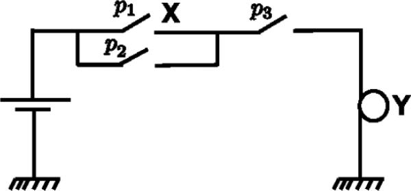
An illustrative example of three switches and a lamp motivating the definition of the proposed necessity measure.

Next, we extend this definition to continuous-valued random variables taking values in the [0, 1] interval. For this purpose, we perform the following algebraic manipulation in the discrete-valued case:

$$\begin{array}{cc}\hfill N(X\to Y)& ={\log }_{2}P(Y=1\mid X=1)-{\log }_{2}P(Y=1\mid X=0)\hfill \\ \hfill & =\sum _{y=0}^1\sum _{x=0}^{1}y(2x-1){\log }_{2}P(Y=y\mid X=x).\hfill \end{array}$$

Extending this to continuous-valued random variables with range [0, 1], we get

$$N(X\to Y)={\int }_0^1{\int }_0^{1}y(2x-1){\log }_2\left(\frac{P_{X,Y}(x,y)}{P_X\left(x\right)}\right)dxdy.$$ (1)

2.2 Partial Necessity Measure

Note that the necessity metric is a bivariate measure, and therefore in multivariate scenarios (i.e. involving more than two random variables) it does not distinguish between direct and indirect necessity. For example, if X is necessary for Y and Y is necessary for Z, then in this bivariate measure X is also necessary for Z, even though the necessity of X to Z is only indirect (or inherited). In order to study the necessity relationships of two random variables after conditioning on the remaining variables in a multivariate scenario, we introduce the following notion of partial necessity, analogous to the partial correlation measures used in undirected networks. Let S be a set of random variables. The partial necessity of X to Y is denoted as N(X → Y|W) where W = S\ {X,Y} represents the remainder of the random variables, and is given by:

$$\begin{array}{cc}\hfill N(X\to Y\mid \mathit{W})& ={\int }_{x,y,\mathit{w}}y(2x-1){\log }_2\left(\frac{p_{XY\mid \mathit{W}}(x,y\mid \mathit{w})}{p_{X\mid \mathit{W}}(x\mid \mathit{w})}\right)p\left(\mathit{w}\right)d\mathit{w}dxdy\hfill \\ \hfill & =E_{\mathit{W}}\left({\int }_{x,y}y(2x-1){\log }_2\left(\frac{p_{XY\mid \mathit{W}}(x,y\mid \mathit{w})}{p_{X\mid \mathit{W}}(x\mid \mathit{w})}\right)dxdy\right).\hfill \end{array}$$

Note that in this formulation, numerical implementation of the partial necessity measure involves computation of the multivariate integration over w. This can be computationally expensive if the number of variables involved is large. In order to simplify the computation, we approximate the expectation by the sample mean as follows:

$$N(X\to Y\mid \mathit{W})\approx \frac{1}{T}\sum _{i=1}^T{\int }_{x,y}y(2x-1){\log }_2\left(\frac{p_{XY\mid \mathit{W}}(x,y\mid \mathit{w}\left(i\right))}{p_{X\mid \mathit{W}}(x\mid \mathit{w}\left(i\right))}\right)dxdy$$ (2)

where w(i) indicates the i^th sample of w, and T represents the number of samples. Note that we first perform kernel density estimation to compute the multivariate distribution of X, Y, W using all of the samples and then compute the conditional distributions at W = w(i) (i.e. at each sample value). This formula is more computationally tractable because it eliminates the p(w) term, and as a result, avoids the high-dimensional multivariate integration over w. Note that in multivariate kernel density estimation, there is an exponential increase in the number of samples as the number of dimensions increases (referred to as the “curse of dimensionality”) [9]. However, in this paper, we are dealing with two-dimensional conditional distributions, which may reduce the sensitivity of our measures to increases in the number of variables (or nodes in a network) relative to the full multivariate distribution, an issue we plan to explore further.

2.3 Interpretation and Properties of the Necessity Measures

In the previous section, a mathematical formulation of the necessity measures was presented. The purpose of this section is to provide an intuitive interpretation and discuss several interesting properties of these measures.

Let X and Y be two binary random variables. In terms of Boolean logic, when X is necessary for Y, Y must be zero whenever X is zero. This condition limits the support of the joint distribution of the two random variables, as illustrated in Fig. 2(a). The black squares represent the support of the joint distribution in the binary-valued case. We can see that the condition that X is necessary for Y requires cases to exist at the bottom-left corner and that no cases may exist at the upper-left corner. Note that when X is one, Y may either be zero or one, as indicated by the presence of black squares in the lower-right and upper-right corners, respectively. Generalizing these statements from binary to continuous-valued random variables results in the joint distribution denoted by the shaded triangle in Fig. 2(a).

Fig. 2.

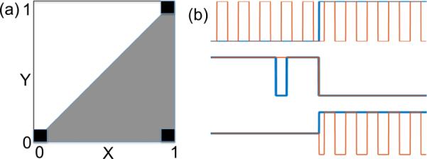
(a) Asymmetry in the joint distribution of two random variables X and Y in the binary-valued case (denoted by black squares) and the continuous-valued case (denoted by the shaded triangle); (b) Hypothetical cases illustrating different cases of correlation and necessity between X (blue) and Y (orange).

The proposed necessity measure can be used to indicate the presence of such asymmetry in the joint distribution of two random variables. A less restrictive form of asymmetry can be observed in the joint distribution of fMRI signals from two different ROIs. A scatter plot of activation of the posterior cingulate gyrus and inferior parietal lobule during resting state fMRI is shown in Fig. 3(a). This example illustrates that there are asymmetric relationships in the activation of these two ROIs, as indicated by the approximately lower-triangular joint distribution in Fig. 3(b).

Fig. 3.

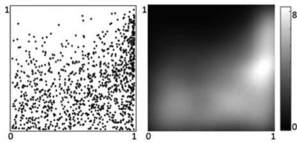
(a) A scatter plot of activation of left posterior cingulate gyrus - dorsal (x-axis) and left inferior parietal lobule - angular gyrus (y-axis) from one of the resting-state fMRI data sets mentioned in Sec. 2.5; (b) Kernel density estimate of the joint distribution.

In order to highlight the difference between correlation and necessity measures, we consider the hypothetical cases shown in Fig. 2(b). The top row shows an example where X (blue) is not necessary for Y (orange) and there is no correlation between X and Y . The middle row shows a case where there is high correlation between X and Y but X is not necessary for Y. Finally, the bottom row shows a case where X is necessary for Y but there is low correlation between X and Y . These examples highlight the differences between necessity and correlation-based network representations. It is also important to point out that the correlation measure is undirected, while our necessity measure can indicate directed relationships. Although the above examples are not realistic representations of fMRI data, similar relationships can exist in the context of fMRI.

Also of interest is the relationship between statistical independence and necessity. When two events A and B are statistically independent, there is no necessity between A and B. Moreover, it can be verified that when A and B are conditionally independent given another event W, there is zero partial necessity between the two. These properties are desirable and are consistent with the intuitive requirement from such a measure.

2.4 Implementation of the Necessity Measures

The numerical implementation of the proposed necessity and partial necessity measures (as given by equations 1 and 2) was performed in MATLAB. The integrations involved in the formulas were discretized using δx = δy = .01 and were computed over [0, 1] × [0, 1]. Accurate estimation of the joint and conditional probability distributions is critical for computation of the necessity measures. We used the Kernel Density Estimation Toolbox for MATLAB (provided by http://www.ics.uci.edu/~ihler/code/kde.html) for the purpose of multivariate joint and conditional probability density estimation. This implementation uses “kd-trees,” a hierarchical representation for point sets which caches sufficient statistics about point locations in order to achieve potential speedups in computation [8].

2.5 Application to fMRI Data

We applied the necessity and partial necessity measures to resting state fMRI data. The dataset used for this paper was provided by the Human Connectome Project (HCP), supported by the WU–Minn Consortium and McDonnell Center for Systems Neuroscience at Washington University [19]. The dataset consisted of 68 healthy participants in the HCP quarter 1 (released online: March 2013) [17]. For each participant, one resting state fMRI session (with left-to-right direction phase encoding) was analyzed. The scan parameters of the resting state fMRI data were: TR, 720 ms; TE, 33.1 ms; flip angle, 52°; field of view, 208 × 180 mm; slice thickness, 2.0 mm; 72 slices; voxels isotropic, 2.0 mm; multiband factor, 8; echo spacing, 0.58 ms; bandwidth (BW), 2290 Hz/Px; time points, 1200 [17].

This data was processed using the HCP preprocessing pipeline, which involves the use of a denoising process that combines independent component analysis (ICA) with an automated component classifier referred to as FIX (FMRIB's ICA-based X-noisifier) [7,17]. ICA is run using FSL's Multivariate Exploratory Linear Optimized Decomposition (MELODIC) with automatic dimensionality estimation. These components are fed into FIX, which determines which components need to be removed from the data. The HCP pipeline uses a grayordinate spatial coordinate system, which allows for combined cortical surface and sub-cortical volume analyses. Additionally, it reduces the storage and processing requirements for high spatial and temporal resolution data.

Note that our necessity measure requires an input in the range [0, 1]. ROI-wise time series were computed by averaging the fMRI signal over each ROI. The fMRI time series for each ROI was normalized by subtracting the mean, taking the absolute value, and then dividing by the standard deviation of the signals from all ROIs in a given network. Using the error function, the resulting signal was transformed to the [0, 1] interval. Using this process, we computed the necessity measures between each pair of ROIs in a given network. For the analysis presented in this paper, we focused on the default mode network, in particular the following ROIs: (1) Posterior Cingulate Gyrus - Dorsal, (2) Posterior Cingulate Gyrus - Ventral, (3) Inferior Parietal Gyrus - Angular, (4) Inferior Parietal Gyrus - Supramarginal, and (5) Superior Frontal Gyrus. ROIs were defined by the HCP preprocessing pipeline, which uses FreeSurfer.

We also performed significance testing, explained as follows. In these studies, we are interested in comparing the necessity of X to Y with the necessity of Y to X, where X and Y represent the activations of two ROIs. In order to determine significance, we performed a one-sided Wilcoxon rank-sum test. The null hypothesis for this test is that necessity of X to Y is equal to that from Y to X in the study population. Rejection of the null hypothesis indicates that necessity of X to Y is greater than the necessity of Y to X, which suggests ascendancy of X over Y in the network. Note that this one-sided test does not consider the possibility that the necessity of Y to X is greater than the necessity of X to Y . To account for this possibility, we also performed hypothesis testing in the opposite direction (i.e. by exchanging X and Y ). In the case of multiple ROIs, all pairwise necessity measures were computed and significance testing was performed in both directions for each pair. Multiple hypothesis correction was performed using false discovery rate (FDR = 0.05) with the Benjamin Hochberg procedure [1].

3 Results

We used the proposed necessity measures to determine the presence of hierarchy and asymmetry of brain interactions during resting state. First, we validated our measures using a simulation based on a model of directed interaction. The simulation demonstrates how partial necessity can distinguish between direct and indirect interactions. We then performed ROI-wise analysis on resting state fMRI data to study connectivity and directed interactions in the default mode network.

3.1 Simulation Based on a Model of Directed Interaction

In this section, we present a simulation to validate the proposed necessity and partial necessity measures. First, consider the following motivating example. Let C be the central hub in a network consisting of two other regions A and B, where we restrict the three variables to be binary-valued (1 indicating activation and 0 indicating inactivation). Suppose we model C as the maximum of A and B. In this case, if C is inactive, then both A and B must be inactive, indicating that activation of C is necessary for activation of A and B. Although this example restricts the variables to be binary-valued, we can extend this concept to the continuous-valued case, as illustrated by the following simulation. We selected three fMRI time series signals, each from a different ROI, and converted them to signals with range [0,1], as explained in Sec. 2.5. These signals are represented by X, W₁, and W₂. We then computed Y = max(X, W₁) and Z = max(Y, W₂), where we took the maximum at each time instant. We then analyzed the connectivity between X, Y , and Z. Intuitively, one would expect activation of Z to be necessary for activation of Y , and activation of Y to be necessary for activation of X. The venn diagram in Fig. 4(a) depicts this subset/superset relationship, with Z being a superset of Y , and Y being a superset of X. We studied the connectivity using the necessity and partial necessity measures, with a one-sided Wilcoxon rank-sum test as a test of significance, as explained in Sec. 2.5. Note that for a given pair of ROIs, say X and Y, we compared the values of N(X → Y ) and N(Y → X), and reported the difference when there is significance. Figs. 4(b) and (c) show block diagrams that illustrate the network connectivity, analyzed using the necessity and partial necessity measures, respectively. The arrows indi cate necessity (e.g. Y is necessary for X), with the number next to the arrow indicating the difference between the two necessity values. As expected, we can see that Z is necessary for Y, and Y is necessary for X. However, the necessity measure also shows a connection between Z and X, which is misleading because this is an indirect interaction. When we compute the partial necessity measure, only the direct interactions are found. Thus, when we are only interested in direct interactions, partial necessity may be the preferred analytical measure.

Fig. 4.

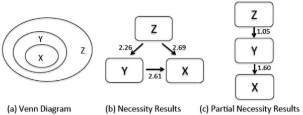
Simulation of Directed Interaction. (a) Venn diagram illustrating the set relationship between random variables X, Y, and Z. Figs. (b) and (c) are block diagrams illustrating the connectivity between X, Y, and Z, using the necessity and partial necessity measures, respectively.

3.2 Analyzing Connectivity and Directed Interactions in the Default Mode Network

We used the proposed necessity measures to study connectivity and directed interactions in the default mode network for both the left and right hemispheres. We restricted our analysis to the following ROIs: (1) Posterior Cingulate Gyrus - Dorsal (PCG-D), (2) Posterior Cingulate Gyrus - Ventral (PCG-V), (3) Inferior Parietal Gyrus - Angular (IP-AG), (4) Inferior Parietal Gyrus - Supra-marginal (IP-SMG), and (5) Superior Frontal Gyrus (SFG). Studies have shown that the posterior cingulate cortex forms a central node in the default mode network [10,3]. Fig. 5 shows a plot of the difference between the necessity of PCG-D to IP-AG and the necessity of IP-AG to PCG-D across the study population. Results are shown for the necessity and partial necessity measures. In both cases, the difference is consistently greater than zero across the subjects, indicating that there is asymmetry in the interaction of these two ROIs. In the following study, we compared our proposed necessity and partial necessity measures to the popularly used correlation and partial correlation measures. We computed all four measures and performed a one-sided Wilcoxon rank-sum test as a test of significance, as explained in Sec. 2.5. Figs. 6(a) and (b) show block diagrams that illustrate the connectivity of the network, analyzed using the necessity and partial necessity measures, respectively. Each block represents an ROI in the network and each arrow indicates a necessity relationship between a pair of ROIs with the number next to the arrow representing the difference between the two necessity values (averaged over the subjects). Similar block diagrams were generated for the correlation and partial correlation measures, shown in Figs. 6(c) and (d), respectively. In the case of the necessity measures, we can see that the majority of the arrows are originating from the PCG. This indicates that activation of the PCG is necessary for activation of the other ROIs in the network, thus supporting the notion that the PCG is a central hub in the default mode network. However, this is not evident from the undirected correlation and partial correlation measures. Also, since the partial necessity measure shows the same connectivity as the necessity measure, this suggests that all of the necessity relationships are direct.

Fig. 5.

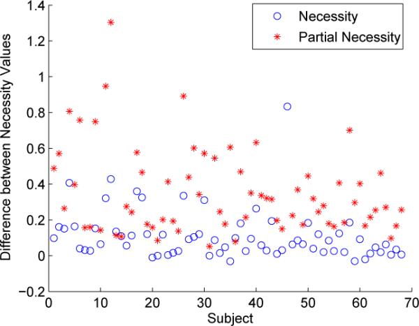
Plot of the differences between the two necessity values (i.e. necessity of PCGD to IP-AG minus necessity of IP-AG to PCG-D) across the study population. Corresponding results for partial necessity are also shown.

Fig. 6.

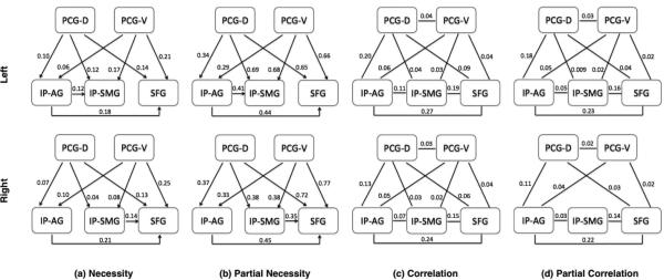
Study of connectivity and directed interactions in the default mode network. We studied connectivity in the default mode network using four measures: (a) Necessity, (b) Partial Necessity, (c) Correlation, and (d) Partial Correlation. The ROIs we studied are as follows: PCG-D = Posterior Cingulate Gyrus - Dorsal; PCG-V = Posterior Cingulate Gyrus - Ventral; IP-AG = Inferior Parietal Lobule - Angular Gyrus; IP-SMG = Inferior Parietal Lobule - Supramarginal Gyrus; SFG = Superior Frontal Gyrus. The top and bottom rows illustrate connectivity in the left and right hemispheres, respectively. The results indicate that the posterior cingulate gyrus plays a central role in the default mode network, which is consistent with the literature.

4 Discussion and Conclusion

We presented a measure of necessity and partial necessity for exploring asymmetric brain interactions during resting state. These measures are particularly useful in the context of fMRI data analysis because they do not depend on time lag information. We validated our measures using a simulation based on a model of directed interaction. Also, we used our measures to study connectivity in the default mode network. Fransson et al. (2008), and others, have conjectured that the posterior cingulate gyrus plays a central role in the default mode network [3,10]. Preliminary results from the necessity measures indicate that activation of the posterior cingulate gyrus is necessary for activation of other ROIs in the network, thus supporting the notion that this region acts as a central hub. While the proposed necessity measures depict subset relationships indicative of a hierarchy of brain activations, it is important to point out that the necessity measures do not indicate a cause-effect relationship. However, ascendancy has been effectively used as a surrogate for causality in previous studies [14,18]. One limitation of the necessity measures is that they use fMRI signal intensities scaled to the [0, 1] interval as a measure of activation. As a result, the necessity measures can be sensitive to the preprocessing pipeline. We will explore the impact of preprocessing on the necessity measures in future studies. Another limitation is that the necessity measures do not take into consideration neurophysiological properties, such as the characteristics of the hemodynamic response and neuromuscular coupling. Also, the partial necessity measure requires computation of multivariate joint distributions and may become increasingly unstable with increasing dimension. We did however investigate the stability of the partial measure using bootstrapping. While within-subject variance increased relative to the non-partial measure, there was still sufficient consistency across subjects, as illustrated in Fig. 5, to detect statistically significant directed interactions.

References

- 1.Benjamini Y, Yekutieli D. The control of the false discovery rate in multiple testing under dependency. Annals of statistics. 2001:1165–1188. [Google Scholar]
- 2.Burge J, Lane T, Link H, Qiu S, Clark VP. Discrete dynamic bayesian network analysis of fmri data. Human brain mapping. 2009;30(1):122–137. doi: 10.1002/hbm.20490. [DOI] [PMC free article] [PubMed] [Google Scholar]
- 3.Fransson P, Marrelec G. The precuneus/posterior cingulate cortex plays a pivotal role in the default mode network: Evidence from a partial correlation network analysis. Neuroimage. 2008;42(3):1178–1184. doi: 10.1016/j.neuroimage.2008.05.059. [DOI] [PubMed] [Google Scholar]
- 4.Friston KJ. Functional and effective connectivity in neuroimaging: a synthesis. Human brain mapping. 1994;2(1-2):56–78. [Google Scholar]
- 5.Friston KJ, Harrison L, Penny W. Dynamic causal modelling. Neuroimage. 2003;19(4):1273–1302. doi: 10.1016/s1053-8119(03)00202-7. [DOI] [PubMed] [Google Scholar]
- 6.Friston KJ, Kahan J, Biswal B, Razi A. A dcm for resting state fmri. NeuroImage. 2014;94:396–407. doi: 10.1016/j.neuroimage.2013.12.009. [DOI] [PMC free article] [PubMed] [Google Scholar]
- 7.Glasser MF, Sotiropoulos SN, Wilson JA, Coalson TS, Fischl B, Andersson JL, Xu J, Jbabdi S, Webster M, Polimeni JR, et al. The minimal preprocessing pipelines for the human connectome project. Neuroimage. 2013;80:105–124. doi: 10.1016/j.neuroimage.2013.04.127. [DOI] [PMC free article] [PubMed] [Google Scholar]
- 8.Gray AG, Moore AW. Very fast multivariate kernel density estimation via computational geometry. Joint Stat. Meeting. 2003.
- 9.Hwang JN, Lay SR, Lippman A. Nonparametric multivariate density estimation: a comparative study. Signal Processing, IEEE Transactions on. 1994;42(10):2795–2810. [Google Scholar]
- 10.Leech R, Braga R, Sharp DJ. Echoes of the brain within the posterior cingulate cortex. The Journal of Neuroscience. 2012;32(1):215–222. doi: 10.1523/JNEUROSCI.3689-11.2012. [DOI] [PMC free article] [PubMed] [Google Scholar]
- 11.Mclntosh A, Gonzalez-Lima F. Structural equation modeling and its application to network analysis in functional brain imaging. Human Brain Mapping. 1994;2(1-2):2–22. [Google Scholar]
- 12.Mill JS. A System of Logic Ratiocinative and Inductive: Boeing a Connected View of the Principales of Evidence and the Methods of Scientific Investigation. Bombay: 1906. [Google Scholar]
- 13.Mumford JA, Ramsey JD. Bayesian networks for fmri: A primer. Neuroimage. 2014;86:573–582. doi: 10.1016/j.neuroimage.2013.10.020. [DOI] [PubMed] [Google Scholar]
- 14.Patel RS, Bowman FD, Rilling JK. A bayesian approach to determining connectivity of the human brain. Human brain mapping. 2006;27(3):267–276. doi: 10.1002/hbm.20182. [DOI] [PMC free article] [PubMed] [Google Scholar]
- 15.Ragin CC. Fuzzy-set social science. University of Chicago Press; 2000. [Google Scholar]
- 16.Roebroeck A, Formisano E, Goebel R. Mapping directed influence over the brain using granger causality and fmri. Neuroimage. 2005;25(1):230–242. doi: 10.1016/j.neuroimage.2004.11.017. [DOI] [PubMed] [Google Scholar]
- 17.Smith SM, Beckmann CF, Andersson J, Auerbach EJ, Bijsterbosch J, Douaud G, Duff E, Feinberg DA, Griffanti L, Harms MP, et al. Resting-state fmri in the human connectome project. Neuroimage. 2013;80:144–168. doi: 10.1016/j.neuroimage.2013.05.039. [DOI] [PMC free article] [PubMed] [Google Scholar]
- 18.Smith SM, Miller KL, Salimi-Khorshidi G, Webster M, Beckmann CF, Nichols TE, Ramsey JD, Woolrich MW. Network modelling methods for fmri. Neuroimage. 2011;54(2):875–891. doi: 10.1016/j.neuroimage.2010.08.063. [DOI] [PubMed] [Google Scholar]
- 19.Van Essen DC, Smith SM, Barch DM, Behrens TE, Yacoub E, Ugurbil K. The wu-minn human connectome project: an overview. Neuroimage. 2013;80:62–79. doi: 10.1016/j.neuroimage.2013.05.041. [DOI] [PMC free article] [PubMed] [Google Scholar]
- 20.Wu X, Li J, Yao L. Neural Information Processing. Springer; 2012. Determining effective connectivity from fmri data using a gaussian dynamic bayesian network. pp. 33–39. [Google Scholar]