Quantifying the uncertainty in heritability

Abstract

The use of mixed models to determine narrow-sense heritability and related quantities such as SNP heritability has received much recent attention. Less attention has been paid to the inherent variability in these estimates. One approach for quantifying variability in estimates of heritability is a frequentist approach, in which heritability is estimated using maximum likelihood and its variance is quantified through an asymptotic normal approximation. An alternative approach is to quantify the uncertainty in heritability through its Bayesian posterior distribution. In this paper, we develop the latter approach, make it computationally efficient and compare it to the frequentist approach. We show theoretically that, for a sufficiently large sample size and intermediate values of heritability, the two approaches provide similar results. Using the Atherosclerosis Risk in Communities cohort, we show empirically that the two approaches can give different results and that the variance/uncertainty can remain large.

Introduction

Intuitively, heritability reflects the idea that traits such as height, weight or disease status are shared within families as a result of shared genetics rather than shared environment. More formally, heritability represents the proportion of the total variance of a given trait that is attributable to genetics.¹ The general term ‘heritability' can be used to refer to either of two more specific types: broad-sense or narrow-sense heritability. Broad-sense heritability refers to the proportion of trait variation that can be attributed to all types of genetic effects, including dominance, epistatic interaction and additive effects. Narrow-sense heritability refers to the proportion of variance accounted for by only additive genetic effects. It is the latter which is of most current interest, as there is substantial evidence that most trait variation introduced by genetics is additive.²

Traditionally, narrow-sense heritability has been estimated using specific family designs.¹ More recently, researchers have used restricted maximum-likelihood (REML) solutions for a linear mixed model (LMM) in conjunction with single-nucleotide polymorphisms (SNPs) to get a coarse sense of this quantity.³ One important issue is that this approach estimates the heritability tagged only by the SNPs used, which is a downwardly biased estimate of narrow-sense heritability. This biased estimate has been referred to as SNP, chip and pseudo- heritability,^{4, 5} although these terms can be confusing, as they do not distinguish between a narrow-sense and broad-sense estimate of heritability. Herein, we shall use ‘SNP heritability' to refer to this estimate of narrow-sense heritability.

Point estimates can be misleading, so researchers have begun to characterize the variance of such estimates. For example, Yang et al.⁶ estimate the variance of such estimates by using an asymptotic Gaussian approximation of the maximum-likelihood estimator for SNP heritability. An apparent problem with such an approach is that SNP heritability is bounded between zero and one, making symmetric distributions such as the Gaussian distribution unsuited to describe SNP heritability close to either extreme. As an alternative to this frequentist-based approach, one may quantify the uncertainty in SNP heritability through its Bayesian posterior distribution. In this approach, the probability distribution of SNP heritability is estimated by combining both prior beliefs about SNP heritability with the information from observed data. Although Bayesian methods have been proposed to evaluate heritability,⁷ the usefulness of the Bayesian approach to quantify the uncertainty in heritability has yet to be fully explored.

Here, we develop the Bayesian approach for representing the uncertainty in SNP heritability and show how the posterior distribution can be determined at a low computational cost. We compare this approach to the frequentist-based approach both theoretically and empirically. Using the Atherosclerosis Risk in Communities (ARIC) cohort, we show that, for large sample sizes, the two approaches typically give similar results. However, we also find that the two approaches can give different results, that the variance/uncertainty in SNP heritability remains large and that the variance/uncertainty of the parameter often is not approximated well by a normal distribution.

Materials and methods

As mentioned, we used genotype and phenotype samples from the ARIC cohort.⁸ We used quality-control standards similar to those performed by Yang et al.³ We considered 706 949 SNPs from the autosomes and the X chromosome. SNPs with an estimated genotyping error rate of >0.01 were excluded from the analysis. Genotyping error rates were estimated per SNP by using a set of 343 duplicate arrays. Finally, we exclude SNPs with a missing rate >2% or with minor allele frequency <1% and any SNPs failing Hardy-Weinberg equilibrium with P<1e-3. This quality control procedure was conducted separately for each race and sex category, and then a final set of SNPs was obtained by intersecting the resulting sets. The final number of autosomal SNPs included in the analysis were 346 565. On the sample level, we excluded individuals with sex inconsistencies determined by X chromosome heterozygosity.⁹ We also removed individuals with a missing call rate >2%. Principal components analysis was used in order to identify and remove individuals of non-European descent. This left a total of 12 636 individuals (4481 Caucasian males, 5057 Caucasian females, 1159 African American males and 1939 African American females). The sample size used for a given phenotype varied, however, because of missing values. Additionally, for each phenotype, individuals were pruned from the set so that no two pairs of individuals were closely related. In particular, individuals were pruned such that no pair of individuals i and j have a value Kij in the kinship matrix >0.025, as in Yang et al.³ This was done on a per phenotype basis, so as to maximize the potential sample size for each phenotype.

We used five continuous phenotypes from the ARIC cohort: height, weight, body mass index, vonWillebrand factor, and QT interval (QTi). Detailed information about these phenotypes can be found at http://www2.cscc.unc.edu/aric/. All phenotypes were age corrected by a smooth non-linear multiplicative function in the form of a maximum-likelihood fit of a Gaussian process to the logarithm of the phenotype, with a squared-exponential covariance function computed on age.¹⁰

Results

SNP heritability

A trait y can be decomposed into a fixed mean μ, a random genetic effect G and a random environmental effect E.³ For the moment, let us assume that each individual in the study has been genotyped at the variants known to be causal for this particular trait. We use an LMM for the likelihood of y. Assuming the variants act linearly and additively, G_n, the genetic effect for individuals n=1,…,N, can be written as 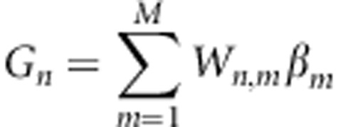, where W_n,m represents the normalized minor allele count for genetic variant m in individual n such that E[W_n,m]=0 and var(W_n,m)=1, and β_m represents the additive effect attributed to this variation. (This choice of normalization reflects the general prior observation that minor allele frequency and effect size are roughly inversely related.¹¹) In matrix notation, we have

where μ is an offset that may include covariates. We assume that the effect vector β is random with 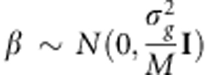. Therefore, , where the matrix K is a kinship matrix.¹² We also assume that the environmental effects attributed to each individual can be represented by independent Gaussian noise, . Consequently, we obtain

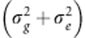
Given this LMM, the narrow-sense heritability of a trait, defined as the heritability attributed to additive genetic effects and denoted as h², equals the ratio of the genetic trait variance 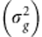to the total trait variance (σ²) or, equivalently, the sum of the genetic variance and the residual error variance ¹:

As mentioned, we typically do not know the causal variants. Consequently, the genotyped SNP markers are often used as a proxy for the causal variants, knowing that the resulting estimates of heritability, often referred to as SNP, chip or pseudo- heritability, will be biased downwards due to the potential exclusion of causal variants.³ Herein, we shall use SNP heritability (or h²) to refer to this (narrow-sense) estimate.

The frequentist approach to estimating SNP heritability and its variation

To obtain , a REML estimate of SNP heritability, we substitute the REML estimates for and into Equation 3. We compute these estimates using FaSTLMM,¹³ which for this task has computational time quadratic in the size of the data per phenotype plus a one-time cost of O(N³).

To obtain an estimate of the variance of , we use the Cramer-Rao lower bound.¹⁴ In particular, if we neglect the fact that the REML estimator of heritability is biased due to a bounded parameter space, its sampling distribution becomes asymptotically normal with mean centered at the true parameter and a lower bound for the variance (approximated using the delta method¹⁴) given by

where F(Θ) the expected information matrix with respect to parameters Θ.

The Bayesian approach to SNP heritability and its uncertainty

In the Bayesian approach, we continue to use the LMM and the expression for h² given by Equation 3, but we now view the parameters as uncertain and express our uncertainty over h² with a probability distribution. From Bayes theorem, we have

where p(h²) and p(h²|y) are the prior and posterior distribution for y, respectively, and p(y|h²) is the likelihood of h² given y. To obtain this likelihood, we frist rewrite Equation 2 as follows:

where . Next, we marginalize over σ²:

Now we assume σ² is independent a priori of h², which is possible as 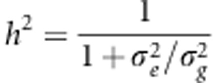(a monotonic function of the ratio of the variances and ) and σ² (the sum of the variances) are variationally independent. Consequently, p(σ²|h²)=p(σ²). Finally, we assume an arbitrary prior for h² and an inverse-Gamma prior for σ², p(σ²)=G⁻¹(σ²|α,γ), where α and γ are hyperparmeters.

The likelihood of h² from Equation 4 equals¹⁵

where St_n(A,B,C) is the multivariate Student-t distribution with mean A, variance B, and degrees of freedom C. Thus, the posterior distribution given by Equation 4 can be determined numerically by evaluating Equation 5 over a grid of possible values for h² and subsequently normalizing the posterior distribution to integrate to 1.

The naive computation of the posterior distribution is computationally expensive, as it would require an O(N³) re-evaluation of Equation 5 for every value of h². However, it is straightforward to use a recent result by Pirinen et al.⁷ and Lippert et al.¹³ in order to reduce the computation to a one-time cost of O(N³) followed by a cost of O(N). In particular, we can rewrite the likelihood from Equation 5 in the following way, where we have let the eigendecomposition of K equal to and factored the eigenvectors from the covariance matrix:

We can then apply the rule PY∼N(PXβ, PΣP^T) for Y∼N(Xβ, Σ) in order to transform the data vector y. Letting y*=H^Ty and X*=H^TX, the likelihood becomes

With this transformation, it is then straightforward to show that the log likelihood can be computed in O(N) given the eigendecomposition of K:

where

and

Comparing the frequentist and Bayesian approaches

In Supplementary Material, we show that both the Bayesian posterior distribution as well as the frequentist distribution asymptotically follow similar normal distributions, where the Bayesian posterior variance is a function of the observed information and the frequentist sampling variance is a function of the expected information. Here, we describe an empirical comparison using (finite) simulated data and real data.

In our simulations, the causal SNPs were known, and all variance was due to linear additive effects, so that our estimates of SNP heritability correspond to estimates of both narrow-sense and broad-sense heritability. We generated two sets of 1000 data sets, one with h²=0.5 and another one with h²=0. Each data set was generated with 500 individuals and 100 SNPs with no population structure and minor allele frequencies drawn uniformly from (0.05,0.4). Using a randomly chosen data set, we calculated the variance of the heritability estimate using both the Bayesian and frequentist approaches and compared these estimates with the empirical variance of all 1000 heritability estimates. For a true heritability of 0.5, both the Bayesian and frequentist approaches resulted in a s.e. of 0.05, matching the empirical s.e. of 0.05. However, for a true heritability of 0, the frequentist s.e. was given by 0.03, whereas the Bayesian s.e. was 0.016, a value much closer to the empirical s.e. of 0.013. This result highlights the fact that, near the boundary of h²=0, the assumptions behind the frequentist estimation procedure break down, resulting in an overestimation of variance.

In our experiments with real data, we compared the two approaches using five phenotypes from the ARIC population cohort.⁸ The total number of available individuals was 13 115, and the total number of available autosomal SNPs was 706 949. We applied extensive filtering (see Methods) to avoid biases in our SNP heritability estimations owing to; for example, low minor allele frequencies or population substructure.³ After filtering the set of individuals and SNPs, we were left with 12 636 total individuals and 346 565 SNPs. We analyzed Caucasians and African Americans separately, and males and females separately, as allelic effects may vary by both sex and race^{16, 17} and, as a result, so will SNP heritability. The maximum sample size for each race–sex cohort is reported in the Methods section, although the actual sample size is phenotype dependent as it varies with the number of missing values. We also analyzed all individuals together, using sex and race as covariates.

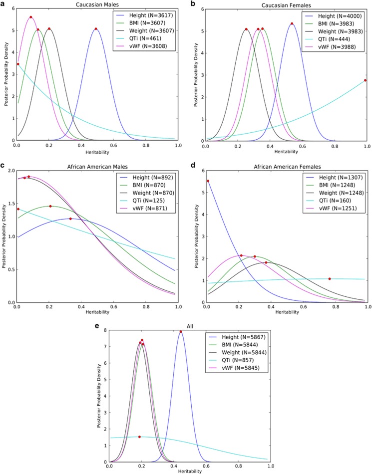
Figure 1 shows graphically the marginal likelihood of the data y given SNP heritability for each phenotype in each sex and race category. Note that, when a uniform prior distribution (that is, a Beta(1,1) distribution) for h² was used, the posterior distribution was just the (normalized) marginal likelihood. Herein, we will use these two interchangeably, in effect assuming such a prior for h². In practice, however, any prior for h² may be used.

Figure 1.

Posterior distributions of SNP heritability for five phenotypes in the ARIC cohort on different subsets of the data. (a) Caucasian males, (b) Caucasian females, (c) African American males, (d) African American females, and (e) the complete data. Posterior distributions were calculated assuming a uniform prior over h² and a relatively flat prior, Γ⁻¹(1,1), over the variance σ². The maximum a posteriori value for heritability is indicated by a red dot. The plots reveal a large degree of uncertainty in heritability.

A comparison of Bayesian and frequentist point estimates are shown in Table 1. Note that some of the frequentist estimates for h² are rather unreasonable. For example, the REML estimate is zero for the height phenotype in African American females. In contrast, the expectation of the Bayesian posterior distribution reflects heritability substantially away from zero. Also, the REML estimates for QTi swing from zero to one depending on the cohort, whereas the Bayesian point estimates do not have such dramatic swings, because the sample size is low and hence these estimates are substantially influenced by the flat prior over h².

Table 1. Summary statistics for heritability posteriors in the ARIC cohort.

Cohort	Phenotype	Sample size	Max. posterior	Posterior expectation	Posterior s.d.	Posterior skewness	Posterior kurtotis	REML estimate	s.e.
Caucasian male	Height	3617	0.49	0.49	0.08	0.03	2.98	0.49	0.08
	BMI	3607	0.13	0.15	0.08	0.4	2.82	0.13	0.09
	Weight	3607	0.2	0.21	0.08	0.15	2.87	0.2	0.08
	QTi	461	0.01	0.25	0.21	1.13	3.8	0	0.61
	vWF	3608	0.09	0.11	0.07	0.6	3.03	0.09	0.08
Caucasian female	Height	4000	0.54	0.54	0.08	0.009	2.98	0.5	0.08
	BMI	3983	0.35	0.35	0.08	0.008	2.99	0.35	0.08
	Weight	3983	0.25	0.25	0.08	0.04	2.94	0.25	0.08
	QTi	444	0.99	0.7	0.23	−0.9	3.09	1	0.63
	vWF	3988	0.33	0.33	0.08	0.03	2.98	0.32	0.08
African American male	Height	892	0.33	0.44	0.26	0.21	2.02	0.25	0.4
	BMI	870	0.21	0.39	0.25	0.42	2.25	0.14	0.38
	Weight	870	0.05	0.33	0.23	0.69	2.72	0.01	0.35
	QTi	125	0.01	0.43	0.28	0.26	1.91	0	1.6
	vWF	871	0.08	0.32	0.23	0.71	2.8	0.03	0.33
African American female	Height	1307	0.01	0.15	0.12	1.32	5.01	0	0.23
	BMI	1248	0.3	0.35	0.19	0.47	2.85	0.28	0.23
	Weight	1248	0.37	0.41	0.21	0.3021	2.53	0.34	0.25
	QTi	160	0.76	0.51	0.28	−0.06	1.83	0.69	1.35
	vWF	1251	0.22	0.3	0.18	0.66	3.07	0.2	0.23
All	Height	5867	0.44	0.44	0.04	0.002	2.99	0.38	0.06
	BMI	5844	0.21	0.21	0.05	0.006	2.99	0.21	0.06
	Weight	5844	0.19	0.19	0.05	0.02	2.97	0.18	0.06
	QTi	857	0.19	0.37	0.22	0.47	2.37	0.17	0.37
	vWF	5845	0.2	0.2	0.05	0.009	2.99	0.13	0.06

Abbreviations: ARIC, Atherosclerosis Risk in Communities; BMI, body mass index; QTi, QT interval; vWF, vonWillebrand factor.

The Bayesian posterior expectation corresponds to the frequentist restricted maximum-likelihood estimate. The Bayesian posterior s.d. corresponds to the frequentist s.e.

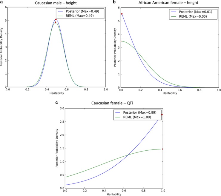
A comparison of Bayesian and frequentist distributions is shown in Figure 2 and Table 1. Under some but not all conditions, the distributions were quite similar. Generally, differences were larger for smaller sample sizes. For example, for the analysis of QTi in African American females (N=160), the s.d. of the Bayesian posterior was 0.28, whereas the s.e. from the frequentist approach was 1.35. In some cases, the posterior distributions were highly non-normal, as can be seen by the higher moments skewness and kurtosis of the distribution in Table 1, which provides additional summary statistics such as the sample size, the maximum a posteriori (MAP) heritability and the expected value given the posterior distribution.

Figure 2.

Comparison of maximum-likelihood estimator distribution with posterior distribution for the examples of (a) height in Caucasian males, (b) height in African American females, and (c) QTi in Caucasian females. Shown are frequentist estimates of the variation of the heritability estimate obtained from GCTA (constrained to values of heritability between 0 and 1) and Bayesian posterior distributions. The area under each distribution is 1. A red dot indicates the maximum of each curve.

Sensitivity to hyperparameters

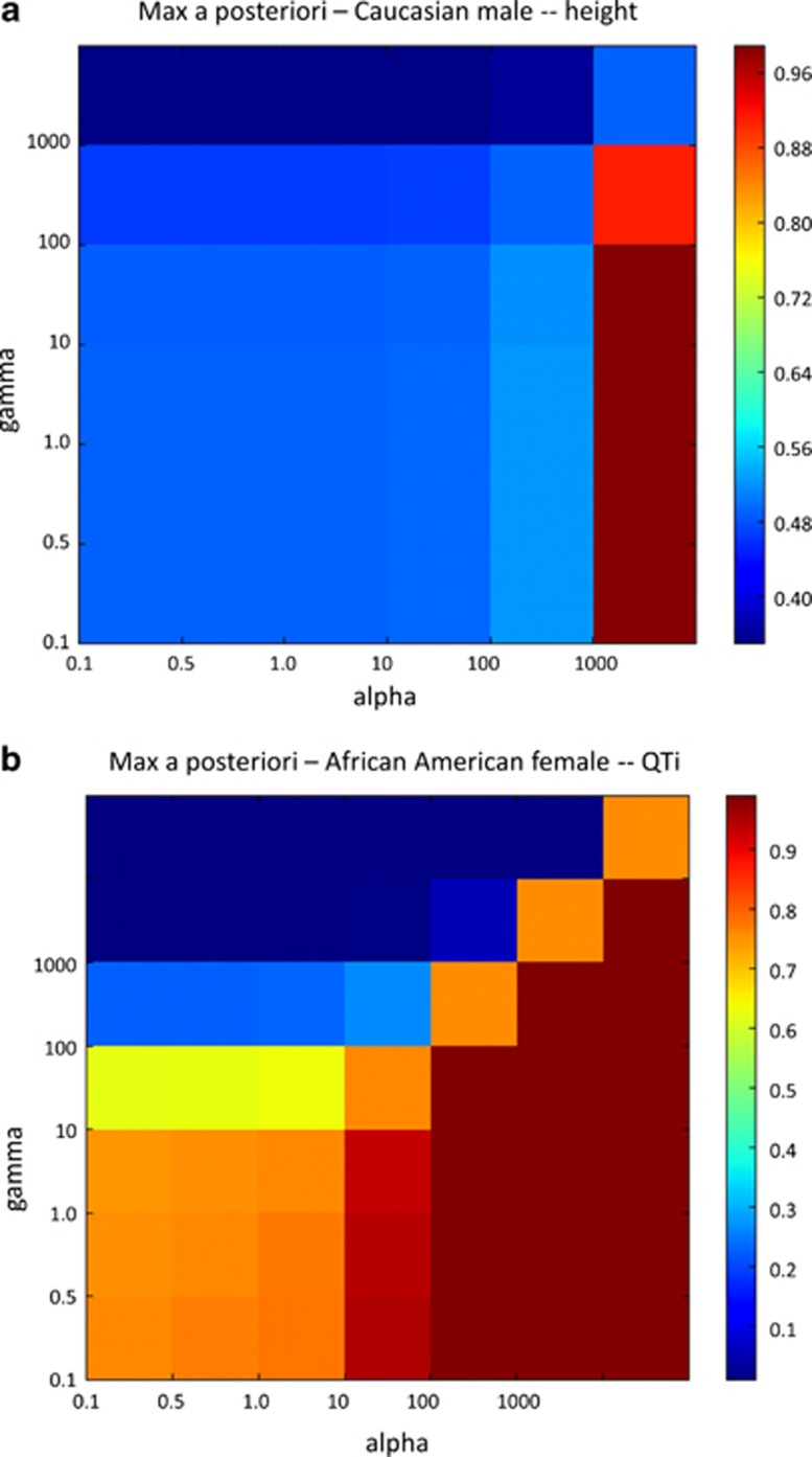
Finally, we evaluated the sensitivity of the posterior distribution to the hyperparameters attributed to the inverse-Gamma distribution on σ². We measured the difference in posterior by evaluating the change in the MAP estimate for heritability, while varying the hyperparameters α and γ. The MAP was evaluated for a range of these parameters from small to large for two data sets: Caucasian male height (N=3617) and African American female QTi (N=160).

Figure 3 shows heatmaps of the MAP for different hyperparameter settings. For male height, we see that the MAP estimates were insensitive to the choice of prior when the hyperparameter values were moderate but were influenced greatly when they became extreme. For the female QTi data, which had a small sample size, the MAP was more sensitive to the prior. Thus, not surprisingly, results should be interpreted cautiously when sample sizes are small.

Figure 3.

Heatmaps showing the change in maximum a posteriori estimates of SNP heritability and the influence of the variance prior. In both heatmaps, MAP values for different hyperparameter settings for the prior distribution on σ² are given. Each grid point represents one hyperparameter setting, and the intensity represents the MAP value, as indicated by the color bar. (a) Height in Caucasian males (sample size is 3617). (b) QTi in African American females (sample size is 160).

Discussion

We have shown how the variation in heritability can be quantified through its Bayesian posterior distribution and how this distribution can be approximated accurately and in a computationally feasible manner. In addition, we have shown how the Bayesian approach for quantifying uncertainty is related to the more commonly used frequentist-based approach, which assumes that the expected spread in heritability estimates can be quantified through a (sometimes problematic) asymptotic Gaussian approximation. We have explained theoretically and shown empirically that these two approaches for quantifying variation in SNP heritability often produce similar results but that even for large sample sizes their results may deviate significantly.

The rather substantial variabilities seen in our experiments on real data highlight the importance of considering such variation. In the current environment, there are many papers focused on achieving point estimates of SNP heritability that are close to those expected from family-based studies. However, as we have shown, the variation in these estimates can often be large and should be taken into account when looking for consistency with family-based studies.

In this paper, we used only continuous phenotypes. However, it is possible to extend this methodology to estimate SNP heritability for case–control phenotypes as in Lee et al.¹⁸ This extension is accomplished with the use of a liability transform, wherein a case-control phenotype is assumed to be determined by an underlying continuous phenotype.

References

- Falconer DS. Introduction to Quantitative Genetics. Ronald Press Co: New York, NY, USA; 1960. [Google Scholar]
- Hill WG, Goddard ME, Visscher PM. Data and theory point to mainly additive genetic variance for complex traits. PLoS Genet. 2008;4:e1000008. doi: 10.1371/journal.pgen.1000008. [DOI] [PMC free article] [PubMed] [Google Scholar]
- Yang J, Benyamin B, McEvoy BP, Gordon S, Henders AK, Nyholt DR, et al. Common SNPs explain a large proportion of the heritability for human height. Nat. Genet. 2010;42:565–569. doi: 10.1038/ng.608. [DOI] [PMC free article] [PubMed] [Google Scholar]
- Speed D, Hemani G, Johnson MR, Balding DJ. Improved heritability estimation from genome-wide SNPs. Am. J. Hum. Genet. 2012;91:1011–1021. doi: 10.1016/j.ajhg.2012.10.010. [DOI] [PMC free article] [PubMed] [Google Scholar]
- Kang HM, Sul JH, Service SK, Zaitlen NA, Kong SY, Freimer NB, et al. Variance component model to account for sample structure in genome-wide association studies. Nat. Genet. 2010;42:348–354. doi: 10.1038/ng.548. [DOI] [PMC free article] [PubMed] [Google Scholar]
- Yang J, Lee SH, Goddard ME, Visscher PM. GCTA: a tool for genome-wide complex trait analysis. Am. J. Hum. Genet. 2011;88:76–82. doi: 10.1016/j.ajhg.2010.11.011. [DOI] [PMC free article] [PubMed] [Google Scholar]
- Pirinen M, Donnelly P, Spencer C. CA. Efficient computation with a linear mixed model on large-scale data sets with applications to genetic studies. Ann. Appl. Stat. 2013;7:369–390. [Google Scholar]
- ARIC Investigators The Atherosclerosis Risk in Communities (ARIC) Stuy: design and objectives. Am. J. Epidemiol. 1989;129:687–702. [PubMed] [Google Scholar]
- Purcell S, Neale B, Todd-Brown K, Thomas L, Ferreira MA, Bender D, et al. PLINK: a tool set for whole-genome association and population-based linkage analyses. Am. J. Hum. Genet. 2007;81:559–575. doi: 10.1086/519795. [DOI] [PMC free article] [PubMed] [Google Scholar]
- Review, P. A., Random, G. & Tech-, C. F. C. E. Rasmussen & C. K. I. Williams, Gaussian Processes for Machine Learning, the MIT Press, 2006, ISBN 026218253X. c 2006 Massachusetts Institute of Technology. www.GaussianProcess.org/gpml ( 2006
- Park JH, Wacholder S, Gail MH, Peters U, Jacobs KB, Chanock SJ, et al. Estimation of effect size distribution from genome-wide association studies and implications for future discoveries. Nat. Genet. 2010;42:570–575. doi: 10.1038/ng.610. [DOI] [PMC free article] [PubMed] [Google Scholar]
- Hayes BJ, Visscher PM, Goddard ME. Increased accuracy of artificial selection by using the realized relationship matrix. Genet. Res. (Camb) 2009;91:47–60. doi: 10.1017/S0016672308009981. [DOI] [PubMed] [Google Scholar]
- Lippert C, Listgarten J, Liu Y, Kadie CM, Davidson RI, Heckerman D. FaST linear mixed models for genome-wide association studies. Nat. Methods. 2011;8:833–835. doi: 10.1038/nmeth.1681. [DOI] [PubMed] [Google Scholar]
- Cramér H. Mathematical Methods of Statistics. Princeton University Press; 1946. [Google Scholar]
- Bernardo J, Smith A. Bayesian Analysis. John Wiley; 1994. [Google Scholar]
- Silventoinen K, Sammalisto S, Perola M, Boomsma DI, Cornes BK, Davis C, et al. Heritability of adult body height: a comparative study of twin cohorts in eight countries. Twin. Res. 2003;6:399–408. doi: 10.1375/136905203770326402. [DOI] [PubMed] [Google Scholar]
- Pan L, Ober C, Abney M. Heritability estimation of sex-specific effects on human quantitative traits. Genet. Epidemiol. 2007;31:338–347. doi: 10.1002/gepi.20214. [DOI] [PubMed] [Google Scholar]
- Lee SH, Wray NR, Goddard ME, Visscher PM. Estimating missing heritability for disease from genome-wide association studies. Am. J. Hum. Genet. 2011;88:294–305. doi: 10.1016/j.ajhg.2011.02.002. [DOI] [PMC free article] [PubMed] [Google Scholar]
Associated Data
This section collects any data citations, data availability statements, or supplementary materials included in this article.