Binocular combination of phase and contrast explained by a gain-control and gain-enhancement model

Abstract

We investigated suprathreshold binocular combination, measuring both the perceived phase and perceived contrast of a cyclopean sine wave. We used a paradigm adapted from Ding and Sperling (2006, 2007) to measure the perceived phase by indicating the apparent location (phase) of the dark trough in the horizontal cyclopean sine wave relative to a black horizontal reference line, and we used the same stimuli to measure perceived contrast by matching the binocular combined contrast to a standard contrast presented to one eye. We found that under normal viewing conditions (high contrast and long stimulus duration), perceived contrast is constant, independent of the interocular contrast ratio and the interocular phase difference, while the perceived phase shifts smoothly from one eye to the other eye depending on the contrast ratios. However, at low contrasts and short stimulus durations, binocular combination is more linear and contrast summation is phase-dependent. To account for phase-dependent contrast summation, we incorporated a fusion remapping mechanism into our model, using disparity energy to shift the monocular phases towards the cyclopean phase in order to align the two eyes' images through motor/sensory fusion. The Ding-Sperling model with motor/sensory fusion mechanism gives a reasonable account of the phase dependence of binocular contrast combination and can account for either the perceived phase or the perceived contrast of a cyclopean sine wave separately; however it requires different model parameters for the two. However, when fit to both phase and contrast data simultaneously, the Ding-Sperling model fails. Incorporating interocular gain enhancement into the model results in a significant improvement in fitting both phase and contrast data simultaneously, successfully accounting for both linear summation at low contrast energy and strong nonlinearity at high contrast energy.

Introduction

Having two frontal eyes confers us with a broader field of view and a spare, in the case of loss; however, as noted by Blake and Fox (1973), the “immediate advantage of having two eyes functioning as one is not obvious. The simple experiment of closing one eye does not result in any dramatic change in the appearance of the visual world.” However, based on work over the last half century, it is now clear that information from the two eyes is combined in the visual nervous system (see Blake & Fox, 1973; Blake, Sloane & Fox, 1981; Blake & Wilson, 2011 for reviews).

Binocular combination has been studied in a wide variety of different tasks including luminance change detection (Cogan, 1987; Cohn & Lasley, 1976), contrast detection (Anderson & Movshon, 1989; Campbell & Green, 1965; Legge, 1984a), contrast discrimination (Baker, Meese, & Georgeson, 2007; Legge, 1981, 1984a; Meese, Georgeson, & Baker, 2006), contrast matching (Baker et al., 2007; Huang, Zhou, Lu, & Zhou, 2011; Huang, Zhou, Zhou, & Lu, 2010; Legge & Rubin, 1981), Vernier acuity (Banton & Levi, 1991), orientation discrimination (Bearse & Freeman, 1994), visual direction (Mansfield & Legge, 1996), and phase perception (Ding & Sperling, 2006, 2007; Huang, Zhou, Lu, Feng, & Zhou, 2009; Huang et al., 2011; Huang et al., 2010).

Several models have been proposed to explain binocular combination. For example, Legge (1984b) proposed a binocular quadratic summation model, C = $\sqrt{{\text{C}}_{\text{L}}^2+{\text{C}}_{\text{R}}^2}$, to account for binocular contrast contours for detection. However, Anderson and Movshon (1989) showed that both added noise and contrast adaptation could alter the shape of binocular contrast contour, which could not be explained by a single channel model like the Legge model. Instead they proposed a multiple-channel model to interpret their data. Cohn and Lasley (1976) also provided evidence that a single channel model was insufficient to predict the detection of changes of luminance. They proposed a two-channel model, one channel for summation and the other for the difference of the two eyes' inputs, to account for binocular combination when the two eyes are presented with luminance changes of the same or opposite interocular polarity.

Interocular inhibition/gain control

From Fechner's paradox, the observation that the perceived brightness or contrast of the binocularly viewed visual field maybe reduced by giving a weak stimulus to one eye, Fry and Bartley (1933) inferred the existence of interocular inhibition in binocular vision. However, the Legge model failed to explain Fechner's paradox because the model does not include any interocular mechanisms. Cogan (1987) included interocular divisive inhibition into the summation channel of a two-channel model for detecting changes of luminance. Kontsevich and Tyler (1994) proposed a two-channel model to explain stereothresholds in the difference channel and binocular contrast summation in the summation channel. They also included interocular inhibition before the summation and difference operations. Li and Atick (1994) proposed a two-channel theory for efficient stereo coding; the two eyes' inputs were first added and subtracted to reduce binocular redundancy and gain control was applied to the summation and difference signals to optimize their sensitivities. Indeed recent models for binocular vision include interocular inhibition to explain binocular visual direction (Mansfield & Legge, 1996), binocular rivalry (Wilson, 2003), dichoptic contrast discrimination (Meese et al., 2006; Meese & Hess, 2004), and the perceived phase of a cyclopean sine wave (Ding & Sperling, 2006, 2007; Huang et al., 2010). Moradi and Heeger (2009) provided fMRI evidence for interocular inhibition and proposed an interocular contrast normalization model to account for their data.

However, models proposed to account for amplitude data (contrast, luminance, or neuronal firing) typically include nonlinear operators to account for the nonlinear transfer function. These nonlinear operators distort phase information when applied to predict the perceived phase of cyclopean sinusoids. To avoid this problem, Ding and Sperling (2006) proposed a model with two paths for each eye: a signal path that is selective for orientation and spatial frequency including only linear operations and a gain-control path that extracts total weighted contrast energy across all orientations and all spatial frequency channels from one eye and exerts gain control to the other eye to account for their binocular combined phase data. They first tried a model with only one layer of interocular contrast gain control (Cogan, 1987; Wilson, 2003). The two eyes inputs are first mutually inhibited and then sum up linearly, i.e.,

where I_L and I_R are the signal inputs to a narrow-band and orientation-selective spatial frequency channel for each eye, and E_L and E_R are the total weighted contrast energy of two eyes' images across all orientations and all spatial frequency channels. However, this one-layer gain-control model violates contrast constraints in binocular combination; at high contrast, the model predicts that the binocular combined contrast would be much smaller than monocular contrast because of strong mutual interocular inhibition in binocular viewing but no inhibition from the other eye in monocular viewing when the other eye is closed. To address this violation, they introduced a second layer of interocular gain control that mutually inhibits the gain control in the first layer, i.e.,

This successfully predicts that the perceived contrast is the same whether one eye is closed or both eyes remain open under normal viewing conditions (at high contrast for long stimulus durations). To test their model, they used an adaptive procedure to measure the perceived phase of a horizontal cyclopean sine wave by indicating the apparent location (phase) of the dark trough of the cyclopean sine wave relative to a black horizontal reference line. They performed six experiments to test the predictions of this two-layer gain-control model: (a) At high contrast, the eye with higher contrast contributes more than predicted by linear summation; (b) at low contrast, the binocular combination behaves like linear summation, and when contrast increases, the behavior of binocular combination becomes more and more nonlinear; (c) the eye with noise will dominate in the combination because, with noise contrast, it has more total contrast. All these predictions were confirmed by their experiments.

However, the contrast constraint proposed by Ding and Sperling (2006) is based on the assumption of perceived contrast constancy, whether both eyes are open (interocular contrast ratio = one) or only one eye is open (interocular contrast ratio = zero or ∞) that comes from everyday experience. This assumption should be confirmed empirically. On the other side, the contrast constraint is not clear when the two eyes are presented with different contrast (interocular contrast ratio ≠ one, zero, or ∞) under normal viewing conditions.

Phase dependence of binocular contrast combination

Huang et al. (2010) used the Ding-Sperling paradigm but measured both the perceived phase and contrast of cyclopean sine waves in different combinations of base contrast, interocular contrast ratios, and interocular phase difference. Under their experimental conditions, they found that perceived contrast was independent of the interocular phase difference while the Ding-Sperling model predicts phase dependent contrast combination. To account for their data, they elaborated the Ding-Sperling model, proposing a multipathway contrast gain-control model (MCM) in which the computation of phase and contrast first shares the same cross-eye contrast-gain controls (Ding-Sperling model) and then separates into two channels for phase and contrast, respectively. In the phase channel, the two eyes' sine waves are added linearly, making the phase computation in MCM identical to the Ding-Sperling model. In the contrast channel, the contrast is first extracted from each eye, raised to the power of an exponent, and then summed together (similar to the Legge model). MCM provided accurate fits to their data under their experimental conditions (high contrast and long stimulus duration). However, the assumption of phase-independent contrast combination is not valid at low contrast, where the contrast combination is dependent on the interocular phase difference (Baker, Wallis, Georgeson, & Meese, 2012). A more elaborate binocular combination model is needed to account for this contrast-dependent phase-dependence of contrast combination.

In this study, in order to provide contrast constraints for model fitting over a broad range of experimental conditions, we developed an adaptive procedure to measure the apparent contrast of a cyclopean sine wave by matching it to the standard contrast of a monocular sine wave. We describe five models for binocular combination and fit the models to both phase and contrast data simultaneously. In order to account for the phase dependence of the perceived contrast of cyclopean sine waves, we included a motor/sensory fusion mechanism in the models. In the Discussion section, we compare and contrast our model with extant models in the literature.

Motor/sensory fusion

Fusional vergence eye movements play a critical role in binocular vision, serving to align the two eyes' images of the same object. The initial disparity vergence responses (DVRs) are elicited at ultra-short latencies in both humans and monkeys when small binocular disparities (<2°) are applied to large textured patterns (Busettini, Fitzgibbon, & Miles, 2001; Masson, Busettini, & Miles, 1997; Sheliga, Chen, Fitzgibbon, & Miles, 2005; Sheliga, Fitzgibbon, & Miles, 2006, 2007). By recording the positions of two eyes with the electromagnetic search coil technique, Sheliga et al. (2007) found that the latencies of DVRs could be as short as ∼70 ms when two horizontal 90° out-of-phase sine-wave gratings were viewed dichoptically.

Sensory fusion, which shares the common primary stimulus—binocular disparity—with motor fusion, also plays an important role in binocular vision. With sensory fusion, misaligned (noncorresponding) retinal images are perceived as single as long as they are within Panum's area (Panum, 1858), and small vergence errors (fixation disparity, FD), can occur without diplopia (Fogt & Jones, 1998a; Ukwade, 2000). Fixation disparity can be measured objectively using eye movement recording (Fogt & Jones, 1998a; Hyson, Julesz, & Fender, 1983) or subjectively by aligning nonius lines (Fogt & Jones, 1998a; Schor, Wood, & Ogawa, 1984; Ukwade, 2000). Hyson et al. (1983) recorded eye motions while their observers viewed a random-dot stereogram and misaligned the stereo images by moving them apart until fusion was lost. They found that the vergence error, the difference between image separation and eye vergence, could be as large as 3°. They postulated that neural remapping occurs during sensory fusion that compensates for the retinal misalignment. Fogt and Jones (1998a) compared fixation disparity obtained by objective and subjective methods by measuring FD as a function of forced vergence. They found that the slope of the objective FD curve was significantly greater than the subjective FD curve, indicating an alteration in retinal correspondence. Richards (1968) noted that the perception of objects in space remains constant regardless of the particular point of fixation. He proposed two spatial remapping models in the lateral geniculate body to explain this apparent stability of objects in visual space. Although the two models were speculative, they provided a framework for spatial remapping in the visual system.

In summary, binocular alignment through motor/sensory fusion may be the first step in binocular combination of two misaligned images. To achieve a stable cyclopean image, the retinal coordinates are remapped through motor/sensory fusion to compensate for any disparity between two eyes' images. However, to date, no extant model of binocular combination includes a motor/sensory mechanism for binocular alignment.

Interocular contrast gain enhancement

In persons with amblyopia, we found evidence for interocular contrast gain enhancement (Ding, Klein, & Levi, 2009) (also see the following article, Ding, Klein, & Levi, 2013). Specifically, we found an absence of suppression from the nondominant eye (NDE) to the dominant eye (DE), which unmasked the NDE-to-DE enhancement, allowing it to become apparent under certain conditions. In order to model this, we first modified the Ding-Sperling model by adding monocular gain control (Ding et al., 2009). Like the first layer of interocular gain control, we assumed that the monocular gain control in one eye was inhibited by the other eye; therefore, one eye's gain would be increased by the other eye because its monocular gain control was suppressed by the other eye. This modified Ding-Sperling model was able to predict the apparent enhancement from NDE to DE and gave much better fits to the perceived phase data of observers with abnormal binocular vision (Ding et al., 2009). However, the modified Ding-Sperling model including monocular gain control failed to fit both phase and contrast data simultaneously. In this and the subsequent article (Ding, Klein, & Levi, 2013), we propose a new modified Ding-Sperling model—the DSKL model by explicitly including interocular enhancement—multiplying the other eye's contrast in one eye's gain operation.

Interstimulus contrast-gain enhancement has been found in center-surround interactions; when the surround contrast was lower than the central contrast, the central contrast was enhanced by its surround contrast (Cannon & Fullenkamp, 1993; Ejima & Takahashi, 1985). Xing and Heeger (2001) proposed a model with multiplicative enhancement to account for this center-surround interaction. Unlike the model proposed by Xing and Heeger (2001) for center-surround interactions, in our model, the gain enhancement from one eye to the other eye also receives the suppression from the other eye.

It is parsimonious to assume that the normal visual system also has interocular gain enhancement that is not apparent because of stronger interocular gain control (suppression). In this article, we extend the Ding-Sperling model with three modifications and compared each of these with the simplified and original Ding-Sperling models in a five-model series with a previous model nested within its following one in fitting both phase and contrast perception data in normal binocular combination. In the Discussion section we also compare our models with several extant models of binocular combination. In the following article (Ding, Klein, & Levi, 2013), we compared these five models with asymmetric model parameters in the two eyes to account for abnormal binocular combination. Individuals with abnormal binocular vision due to strabismus and/or amblyopia provide a special challenge to all models of binocular combination and therefore may be crucial to discerning amongst different models.

Methods

Stimuli and procedures for Experiment 1, measuring the perceived phase of a cyclopean sine wave, are similar to those used in previous studies (Ding & Sperling, 2006, 2007). For Experiment 2, stimuli were identical to Experiment 1 but a contrast matching procedure was used to measure the perceived contrast of a cyclopean sine wave.

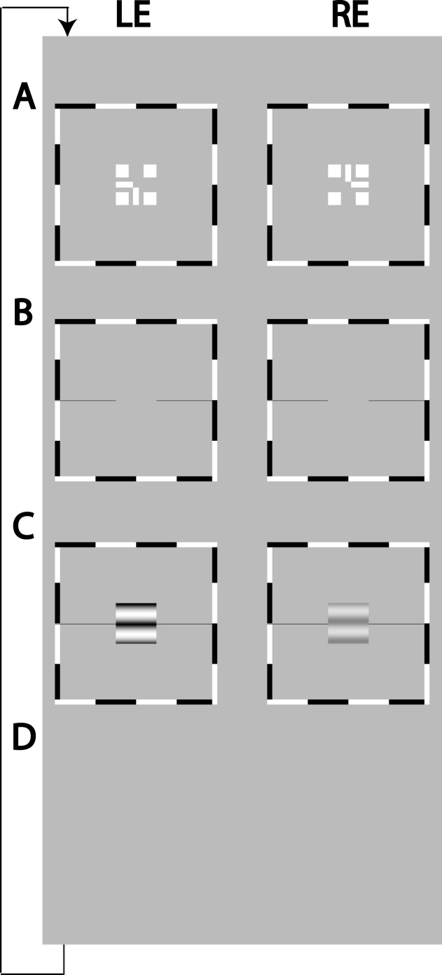
Binocular fusion-assisting frames

Figure 1A shows two frames that were presented to the two eyes, respectively, at the beginning of each trial. The two frames were identical except that the half cross, “7” image without the corner (left in Figure 1A) was presented to the left eye, and the other half cross, “L” image without the corner (right in Figure 1A) was presented to the right eye. With appropriate vergence, a whole cross with a blank square in its center would be perceived. To assist vergence, a high contrast surrounding frame and four squares were also presented binocularly.

Figure 1.

Binocular-fusion-assisting frames and stimuli. (A) A dichoptic nonius cross surrounded by a high contrast frame. (B) A screen with only the surrounding high-contrast frame and reference horizontal lines lasted for 500 ms. (C) Sine-wave gratings presented to the two eyes for 1 s or 117 ms. An observer's task was to indicate the apparent location of the center of the dark stripe in the perceived cyclopean sine-wave grating relative to reference horizontal lines adjacent to its edge. (D) A blank screen of mean luminance waiting for the observer's response.

Stimuli

Horizontal gratings with sinusoidal luminance profiles, I_L = I₀ + m_L cos(2πf_sy + θ_L) and I_R = I₀ + m_R cos(2πf_sy + θ_R), were used as stimuli. I₀ is the luminance of the background and the mean luminance of the sine-wave gratings; f_s is the spatial frequency, identical in both eyes; m_L and m_R are the modulation contrasts of the left- and right-eye sine-wave gratings, respectively; θ_L and θ_R are the corresponding phases. The stimuli were windowed in a rectangular window both spatially (3° × 3°) and temporally (1 s or 117 ms). There were exactly two cycles visible in each eye's sine wave.

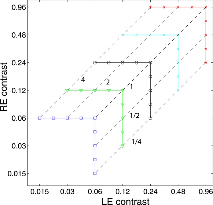
In Experiment 1, we measured the perceived phase of the binocular-combined cyclopean sine wave when the base contrast, m = max{m_L, m_R}, varied from 6% to 96%, interocular contrast ratio, δ = m_R/m_L, varied from ¼ to four, the spatial frequency was 0.68, 1.36, or 2.72 cpd (cycles per degree), and the phase difference, θ = |θ_R – θ_L|, was fixed at 90°. Figure 2 shows the 45 test points of right (RE) versus left eye (LE) contrast at which the perceived phase was measured. Points in one solid curve have the same base contrast m and the points along a dashed line have the same interocular contrast ratio δ that is labeled near the line. For each base contrast, when δ ≤ 1 (vertical solid lines), m_L = m and m_R = δm; when δ > 1 (horizontal solid lines), m_L = m/δ and m_R = m. When δ increases from zero to ∞, the contrast of the LE's grating remains constant at base contrast m while the RE's contrast increases from zero to m (points from bottom to top along a vertical line), and then the RE's contrast remains constant at base contrast m while the LE's contrast decreases from m to zero (points from right to left in a horizontal line).

Figure 2.

Experimental points in RE vs. LE contrast plane. A solid line connects points of the same base contrast (0.06, 0.12, 0.24, 0.48, and 0.96), higher contrast in the two eyes, and a dashed line connects points of the same interocular contrast ratio RE/LE that is labeled near the line in the range from ¼ to 4.

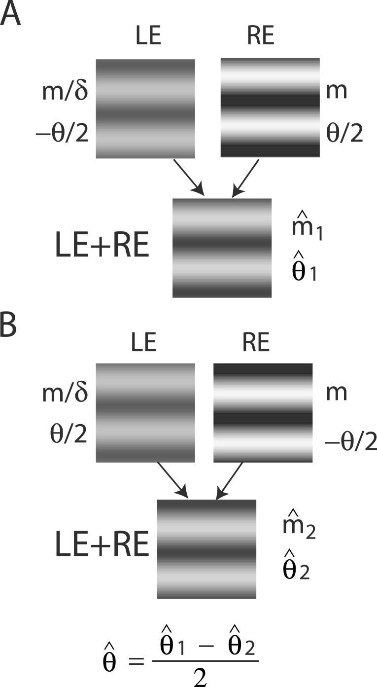
For any given combination of m and δ, there are two displays: (a) the phase of the LE's grating is lower-shifted (θ_L = −θ/2) and the phase of the RE's is higher-shifted (θ_R = θ/2) (Figure 3A); (b) the phase of the LE's is higher-shifted (θ_L = θ/2) and the phase of the RE's is lower-shifted (θ_R = −θ/2) (Figure 3B). For the two displays, two staircases were randomly interleaved to measure the perceived phases, θˆ₁ or θˆ₂, in the cyclopean sine waves (LE + RE) concurrently. When only the LE is presented with a grating (i.e., δ = RE/LE = 0), the perceived phase is the same as in LE's, i.e., θˆ₁ = θ_L = −θ/2 for the display shown in Figure 3A or θˆ₂ = θ_L = θ/2 for the display shown in Figure 3B. On the other hand, when a grating is presented only to the RE (i.e., δ = ∞), the perceived phase is the same as in RE's, i.e., θˆ₁ = θ_R = θ/2 (Figure 3A) or θˆ₂ = θ_R = −θ/2 (Figure 3B). To cancel any possible vertical position bias, the perceived phase is averaged as θˆ = (θˆ₁ − θˆ₂ )/2, which varies from the LE's phase (−θ/2) to the RE's phase (θ/2) when δ increases from zero to ∞.

Figure 3.

Stimulus configurations. The sample stimuli shown in (A) and (B) are for the case when RE/LE = δ > 1.

Stimuli used in Experiment 2 were identical to those in Experiment 1. For both experiments, stimuli were presented on a Sony monitor with a 640 × 480 spatial pixel resolution and 60 Hz vertical refresh rate. The experiments were controlled by a G4 Macintosh running Matlab (MathWorks, Inc.) with the Psychophysics Toolbox extensions (Brainard, 1997; Pelli, 1997). A special circuit (Pelli & Zhang, 1991) was used to yield about 12 bits gray-scale levels. The luminance of the monitor with all pixels set to the minimum value was 7.8 cd/m²; the luminance with all pixels set to the maximum value was 46.0 cd/m². The background level I₀ surrounding the sine-wave gratings was set to 26.2 cd/m², and this was also the average luminance of the sine waves themselves. Displays were viewed in a mirror stereoscope and positioned optically at 68 (0.68 cpd of sine waves), 136 (1.36 cpd of sine waves), or 272 cm (2.72 cpd of sine waves) from the observer.

Procedure

The procedure for Experiment 1 was identical to previous studies by Ding and Sperling (2006, 2007). Each trial began with presentation of a dichoptic nonius cross surrounded by a high contrast frame (Figure 1A). Once the dichoptic cross appeared to be aligned and stable, the observer pressed a key to initiate the trial. Following the key press, a screen with only the surrounding high-contrast frame and reference horizontal lines appeared for 500 ms (Figure 1B), followed by sine-wave gratings presented to the two eyes, respectively, for 1 s or 117 ms (Figure 1C). Stimulus presentation was followed by a blank screen of mean luminance (Figure 1D) until the observer responded. The observer's task was to indicate the apparent location of the center of the dark stripe in the perceived cyclopean sine-wave grating relative to a black horizontal reference line adjacent to its edge. The observer pressed one of two keys to indicate whether the reference line was judged to be above or below the dark cyclopean stripe. After the response, the dichoptic cross reappeared.

For Experiment 2, the procedure was similar to that used in Experiment 1 except having two stimulus intervals, one with a standard contrast (48%, 24%, 12%, or 6%) only presented to the LE and the other with a test contrast presented to both eyes with the interocular contrast ratio varying from trial to trial. Each interval lasted for 1 s or 117 ms and the interstimulus interval was 0.5 s. The observer's task was to judge which interval had the sine wave with higher contrast. At each contrast ratio, two staircases were interleaved to measure the contrast of the test cyclopean sine wave depending on whether the standard contrast was in the first or second interval. The average of these two measurements was calculated as the perceived contrast at that contrast ratio. A black horizontal line was also attached to the side of a sine wave to make the stimulus identical to those used in Experiment 1.

Staircases

An adaptive procedure with many concurrent staircases was used in both experiments. For Experiment 1, within a staircase, the position of the reference line was varied according to the response to the previous trial of that staircase. In each staircase, when the response was “Above,” the reference line was moved down on the next trial of that staircase; when the response was “Below,” the reference line was moved up in the next trial. Each staircase was run for 50 trials. For one run, the spatial frequency, phase difference, and the base contrast were fixed, but interocular contrast ratio varied, i.e., the points in one solid curve in Figure 2 were tested in random order. For each interocular contrast ratio, two staircases were interleaved to measure the perceived phase of the two displays (Figure 3), and the average perceived phase, θˆ = (θˆ₁ − θˆ₂ )/2, was calculated as the dependent variable of the experiment. Typically, for each run, there were 18 concurrent staircases interleaved to measure the perceived phase for nine interocular contrast ratios. Observers JP and MD each ran a total of 3 (Spatial Frequency) × 6 (Base Contrast) × 9 (Contrast Ratio) × 2 (Displays) × 50 (Repeats) = 16,200 trials. Observers CF, CG, KT, and JS each ran a total of 1 (Spatial Frequency) × 3, 4, or 5 (Base Contrast) × 9 (Contrast Ratio) × 2 (Displays) × 50 (Repeats) ≈ 3,600 trials.

For Experiment 2, within a staircase, the contrast of a test sine wave was varied according to the response to the previous trial of the staircase. Each staircase was run for 50 trials. For one run, the spatial frequency, interocular phase difference, and standard contrast were fixed, but interocular contrast ratios were tested in random order. Because of an asymmetry in performance of the two intervals (Nachmias, 2006; Yeshurun, Carrasco, & Maloney, 2008), for each contrast ratio, two staircases were interleaved for the contrast matching task depending on the temporal positions of the standard whether it was in the first or second interval. Indeed, the apparent contrast in the second interval appeared higher (10.7 ± 1.1% across all conditions and observers) than that in the first interval, consistent with Klein's (2001) personal experience. In order to cancel any interval biases, the average test contrast that matches the standard was calculated as the dependent variable of the experiment. There were 22 or 18 concurrent staircases interleaved for each run. Observers JP and MD each ran a total of 3 (Spatial Frequency) × 1 (Standard Contrast) × 1 or 2 (Interocular Phase Difference) × 11 (Contrast Ratio) × 2 (One Staircase for Each Temporal Position of the Standard) × 50 (Repeats) ≈ 5500 trials. Observers CF, CG, KT, and JS each ran a total of 1 (Spatial Frequency) × 4 (Standard Contrast) × 3 (Interocular Phase Difference) × 9 (Contrast Ratio) × 2 (One Staircase for Each Temporal Position of the Standard) × 50 (Repeats) = 10,800 trials.

We fit cumulative Gaussian distributions to the data using maximum likelihood estimation. For Experiment 1, the perceived phase of a cyclopean grating was defined as the point at which the reference line is equally likely to be judged above or below the center of the dark band, i.e., 50% “Above” and 50% “Below” responses. The perceived contrast of the cyclopean grating was defined as the contrast that was equally likely to be judged above and below the standard contrast. A bootstrap method was used to estimate the standard error of the perceived phase and contrast. For each staircase, the total 50 trials were resampled with replacement to get 50 bootstrap trials for a bootstrap session, and the perceived phase or contract was estimated for each bootstrap session; 2000 bootstrap sessions were run in order to estimate the standard error of the perceived phase or contrast.

Observers

Six observers, all in their 20s and with normal or corrected to normal vision, signed the written consent forms and participated in the experiment. Before the experiment, each observer performed one practice session with the sine-wave grating presented to only one eye (control condition) to ensure they understood how to perform the task.

Models

We assume that the perceived cyclopean sine wave has no distortion in phase, and therefore, the signal path in a binocular combination model should only have linear operators. We place all nonlinear operations into a gain control path that modifies the amplitude of the signal before binocular combination. After being modified in their amplitudes, the signals from the two eyes are linearly summed. In order to try to understand binocular combination of phase and contrast, we proposed five models in a series with a previous model nested within its successor to fit the data.

Model 1: Contrast-weighted summation model (simplified Ding-Sperling model)

When contrast energy E is large enough, the constant term “1” in the Ding-Sperling model (Equation 2) can be neglected, and the gain-control model becomes the contrast-weighted summation model, i.e.,

where E_L and E_R are the total weighted contrast energy presented to the two eyes which should be summed over space and time and also over spatial frequency channels and all orientations. In this study, because the stimuli are in a narrow spatial frequency band and have a fixed size and duration at one spatial frequency, the total contrast energy in one channel can be written as

where g_c is a gain-control threshold at which the contrast gain control becomes apparent.

In normal vision, even at low contrast (5%), the contrast energies are much larger than “1” for 1 s stimulus duration, and the contrast-weighted summation model (Equation 3) provides a good fit to the experimental data (Ding & Sperling, 2006 and 2007). However, at short stimulus durations (less than 100 ms), the constant term “1” cannot be neglected because the contrast energy at short durations becomes comparable to “1” (Ding & Sperling 2007). In this study, we asked whether the contrast-weighted summation model can account for both phase and contrast perception simultaneously in binocular combination. Considering the two eyes might have different monocular contrast sensitivities, we introduced contrast attenuation (μ) in the RE, and Equation 3 was rewritten as follows:

Model 2: Ding-Sperling model

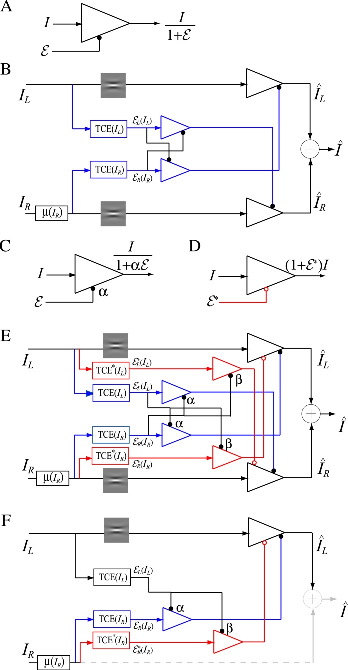
Figure 4A shows a basic unit of contrast gain control: the contrast energy E exerts divisive inhibition to the input I which was repeatedly used in constructing the Ding-Sperling model (Figure 4B) and DSKL (Ding-Sperling-Klein-Levi) model (Figure 4E). The Ding-Sperling model consists of left and right eye channels, each containing two gain control mechanisms: one based on total contrast energy (TCE) in the gain-control layer (blue) which is nonselective for orientation and spatial frequency and the other which is selective along those dimensions in the signal layer (black). The two TCE components exert reciprocal inhibition on one another in the gain-control layers (blue) in proportion to their respective TCE outputs, and the outputs of those TCE components exert gain control on the other eye's selective gain control in the signal layer (black). The outputs are summed linearly to determine the binocular signal.

Figure 4.

Models for binocular combination. (A) The basic unit of contrast-gain control. (B) Ding-Sperling model for binocular combination (Model 2). (C) The basic unit of contrast-gain control with gain-control efficiency of α. (D) The basic unit of contrast gain enhancement. (E) DSKL model (Model 3c). One eye receives both gain control and gain enhancement from the other eye and exerts gain control to the other eye's signal, gain control, and gain enhancement layers separately with different gain-control efficiencies (1, α, and β, respectively). (F) The left eye's output of DSKL model (first summand in Equation 10).

With attenuation (μ) in the RE, the model output is given by

When the left eye's contrast increases, the right eye's gain decreases because of increasing gain control from the left eye, while the left eye's gain increases through decreasing gain control from the right eye (and vice-versa). At high contrast, i.e., m_L >> g_c and m_R >> g_c, the Ding-Sperling model (Equation 6) can be simplified to the contrast-weighted summation model (Equation 5). In order to fit both the phase and contrast data simultaneously, we also fit several variations of the Ding-Sperling model.

Model 3a: Ding-Sperling model with asymmetry between two gain-control layers to the model

In the Ding-Sperling model, one eye is assumed to inhibit the other eye equally in the two layers (black and blue lines in Figure 4B). Generally speaking, however, the gain-control efficiency in the two layers might be different. Figure 4C shows a gain-control operator whose gain-control efficiency is α, which is assumed to be one in both layers for Ding-Sperling model. We first modified the model by adding an asymmetry between the two layers, the gain control and the gain-control of gain control having different gain-control efficiency, i.e.,

where α is the relative gain-control efficiency in the nonselective layer (blue) when the gain-control efficiency (black) in the selective layer is assumed to be one.

Model 3b: Ding-Sperling model with interocular gain enhancement to the model

Studying binocular combination in amblyopic vision (Ding, Klein, & Levi, 2013), we found apparent interocular gain enhancement (IGE); the stimulus in the nondominant eye (NDE) enhanced the dominant eye's (DE's) gain, making the perceived phase further shifted to the DE when the NDE's contrast increased. It is parsimonious to assume that IGE also exists in normal vision but is not apparent because of stronger interocular inhibition. For amblyopic vision, however, because of absent or very weak NDE-to-DE inhibition, the NDE-to-DE gain enhancement becomes apparent. Figure 4D illustrates a gain enhancement operator; its gain is increased by 1 + E* where E* is the contrast energy for gain enhancement. By adding IGE to the model, we have

where

are contrast energy for gain enhancement with gain-enhancement threshold g_e.

Model 3c: Full model with mutual inhibition to a gain enhancement (DSKL model)

This model (the full model) includes a mutual inhibition to the gain enhancement. The model's output is given by

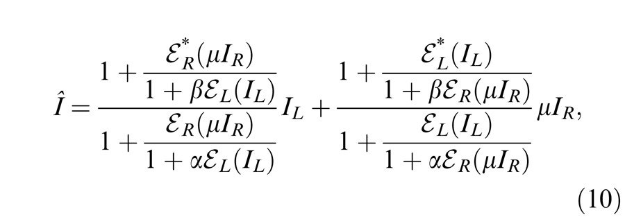where β is the relative gain-control efficiency in the gain control to the gain enhancement. In the full model (Figure 4E), there are three layers for each eyes: (a) the selective signal layer (black) that receives both gain control (black filled circle) and gain enhancement (red open circle) from the other eye and outputs the signal to the binocular summation site; (b) the nonselective gain-control layer (blue) that first extracts and sums image contrast energy across frequency channels and orientations (TCE) and then exerts gain control to the other eye's three layers separately with different gain-control efficiencies (1, α, and β); (c) the gain-enhancement layer that extracts image contrast energy (TCE*) and exerts gain enhancement only to the other eye's signal layer. Figure 4F illustrates the left eye's part of the full model to show how to calculate the left eye's output (the first summand in Equation 10). Before output, the left eye's signal receives gain control from the right eye's gain-control layer that itself receives gain control from the left eye and also the left eye's signal receives gain enhancement from the right eye's gain-enhancement layer that receives gain control from the left eye. The right eye's part in the full model is symmetric to the left eye's in the normal vision.

Asymptote of Models 2 and 3a–c at zero contrast energy

At zero contrast energy, i.e., E_L = 0, E_R = 0, $E_L^{*}$ = 0, and $E_L^{*}$ = 0 no gain control or gain enhancement would be exerted from one eye to the other eye, and Model 2 (Equation 6) and Models 3a–c (Equations 7, 8, 10) become linear summation models, i.e.,

which gives the predictions of black dashed curves in Figures 6 and 7.

Figure 6.

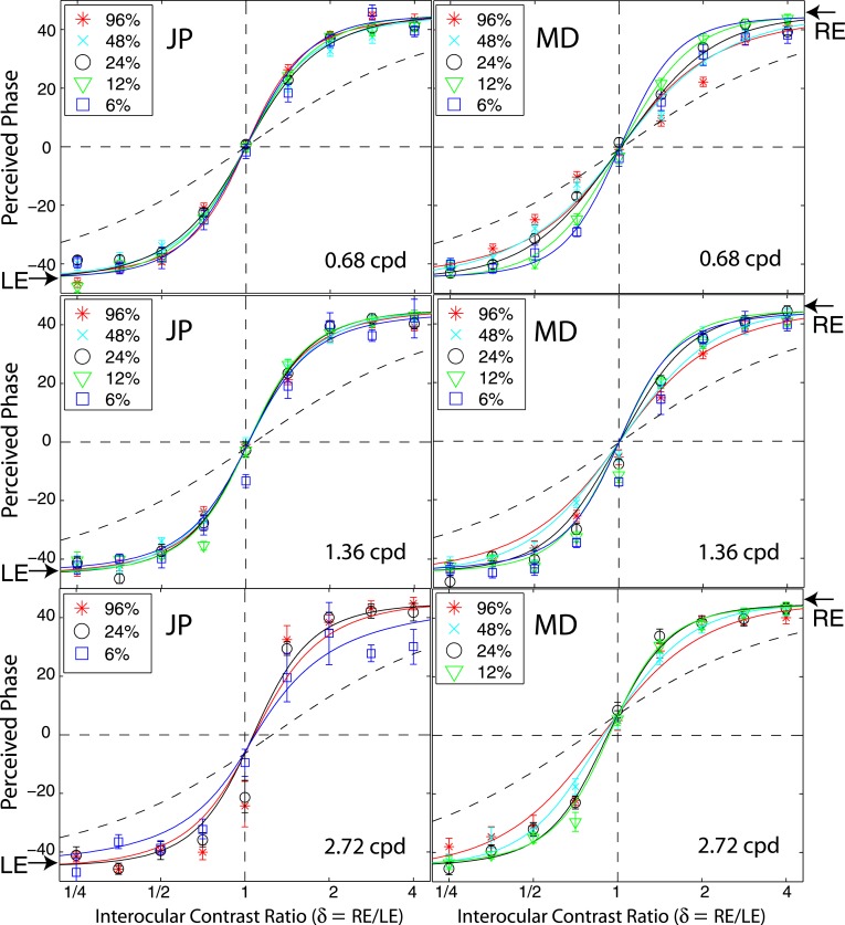
Results of Experiment 1. Perceived phase θˆ of binocular-combined cyclopean sine waves as a function of RE/LE contrast ratio (δ) when the base contrast m is 96% (*), 48% (x), 24% (○), 12% (▿), or 6% (□), and the spatial frequency is 0.68 (top), 1.36 (middle), or 2.72 cpd (bottom). The stimulus duration was fixed at 1 s. The phase difference in the two eyes was fixed at 90°; the arrows on the left side indicate the phase of the LE's sine-wave gratings (−45°), and the arrows on the right side indicate the phase of the RE's (45°). All test points are shown in Figure 2. When δ increased, the perceived phase θˆ shifted from the LE to the RE. When δ ≤ 1 the LE's grating contrast is fixed at the base contrast m′ and the RE's grating contrast δm varies. When δ > 1 , the RE's grating contrast is fixed at m and the LE's grating contrast m/δ varies. The solid curves are the best fits from Model 3c (the DSKL model). The black dashed curve is the prediction from linear summation with attenuation in the RE for ocular imbalanced contrast perception, the asymptote of Models 2 and 3a–c at zero contrast energy.

Figure 7.

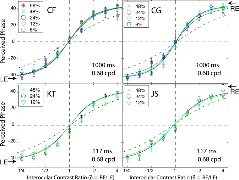
Results of Experiment 1 of four other observers when stimulus spatial frequency was at 0.68 cpd and stimulus duration was 1000 ms for two observers (CG and CF) and 117 ms for another two observers (KT and JS).

Including a motor/sensory fusion mechanism in the model

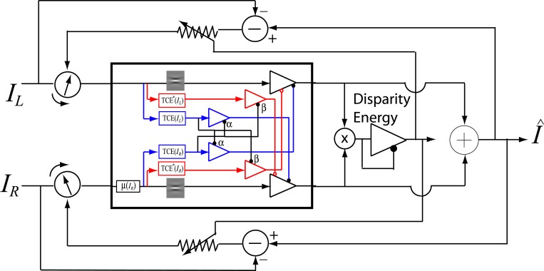
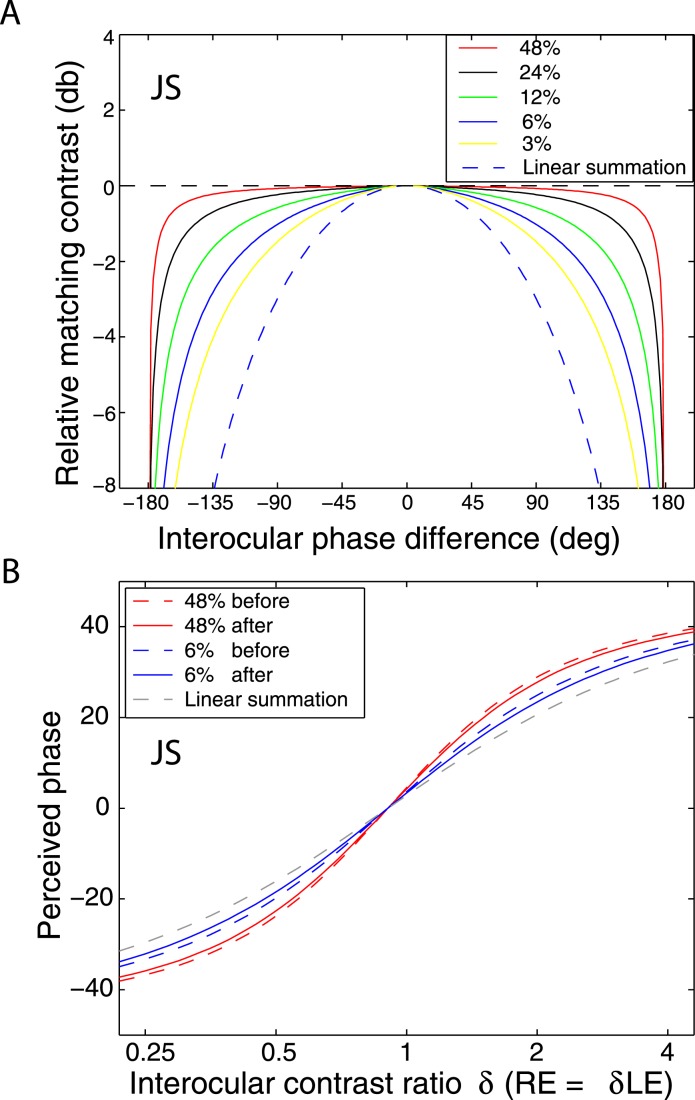
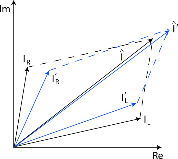
When the two eyes are presented with two images that are identical except for a small offset, motor/sensory fusion may occur to align the two eyes' images. In order to explain the phase dependence of contrast combination, we include a motor/sensory fusion mechanism (Figure 5) in our models. After remapping of corresponding points through motor/sensory fusion, the interocular phase difference in retinal coordinates becomes smaller than that in physical coordinates. In Figure 5, after the interocular interaction, the monocular outputs are combined in two different ways: (a) vector linear summation to produce a cyclopean sine wave, giving form perception such as contrast and phase and (b) vector cross multiplication to extract disparity energy, driving the two monocular misaligned sine waves towards the cyclopean phase (Equation A6) through eye movements and/or remapping of corresponding points in the two eyes. We suppose that the extracted disparity energy first undergoes gain control and then drives motor/sensory fusion that shifts the two monocular phases towards the cyclopean phase until reaching a steady state. High disparity energy could shift monocular phases to be perfectly aligned with the cyclopean phase. Generally, the shifted phase in one eye is a fraction of the phase difference between the sine waves of that eye and the cyclopean eye (Equation A7). After motor/sensory fusion, the perceived contrast of the cyclopean sine wave becomes higher than before fusion while its perceived phase remains almost unchanged (Figure 17B).

Figure 5.

A remapping mechanism for motor/sensory fusion. After interocular interactions, the two eyes inputs are combined in two different ways: (a) vector linear summation to produce a cyclopean image from which form perceptions, such as position (phase) and contrast (amplitude), are perceived; (b) vector cross multiplication to calculate disparity energy for motor/sensory fusion. The disparity energy is supposed to go through a gain control first and then to drive each eye's sine wave towards the cyclopean sine wave by a phase angle of the fraction of the phase difference between that eye and the cyclopean eye.

Figure 17.

Simulation results of the DSKL model (Model 3c) for binocular combination. (A) Simulation of contrast combination as a function of interocular phase difference at several standard contrast levels (Baker et al., 2012) when two sine waves with identical contrast but with different phases were presented to the two eyes. (B) Simulation of phase combination before (dashed colored curves) and after (solid colored curves) motor/sensory fusion when the base contrast is 6% (blue) or 48% (red). The linear summation curve is also shown (dashed grey curve).

Below we show how the predictions of these models fit both the perceived phase and contrast data for a cyclopean sine wave (The Appendix shows how these predictions were deduced.).

Results

Experiment 1: Phase combination

Figure 6 shows how perceived phase (θˆ) of a cyclopean grating varies as a function of the interocular contrast ratio (δ). The (physical) phase difference in two eyes was fixed at 90° (θ_L = −45° and θ_R = 45° indicated by arrows on the sides of Figure 6), the base contrast was 96% (*), 48% (×), 24% (○), 12% (▿), or 6% (□), and the spatial frequency was 0.68 (top), 1.36 (middle), or 2.72 cpd (bottom). When the interocular contrast ratio δ increased, the perceived phase of the cyclopean sine waves shifted systematically from the left eye's phase (−45°) to the right eye's phase (45°). The results are consistent with previous studies (Ding & Sperling, 2006, 2007). The solid curves are the best fits from the DSKL model (Model 3c). The black dashed curve is the prediction from algebraic (linear) summation of two eyes' sine waves with attenuation in the right eye for ocular imbalanced contrast perception (the asymptote of Models 2 and 3a–c at zero contrast energy—see Models section). All data points except equal-physical-contrast (δ = 1) points are shifted away from this linear-summation line, biased to the eye presented with stronger contrast (to the LE when δ < 1 and to the RE when δ > 1). This bias toward the eye with stronger contrast (beyond linear summation) demonstrates interocular contrast gain control. At the lowest spatial frequency (0.68 cpd), all curves (solid and dashed) intercept almost at the same point, with almost no perceived phase shifted at equal physical contrast (δ = 1, dashed vertical line), indicating almost no eye-bias or balanced vision when the two eyes are presented with identical contrast. However, at the highest spatial frequency (2.72 cpd), both observers showed some eye bias; JP biased toward the LE and MD biased toward the RE.

Figure 7 shows results of Experiment 1 for four other observers with spatial frequency of 0.68 cpd; two at the standard stimulus duration (1000 ms), and two at a stimulus duration of 117 ms, too brief for eye-movements. These four observers also performed Experiment 2 at multiple contrast levels and multiple interocular phase differences. The DSKL model was used to fit the data from the two experiments simultaneously.

Experiment 2: Contrast combination

Contrast combination at different spatial frequencies

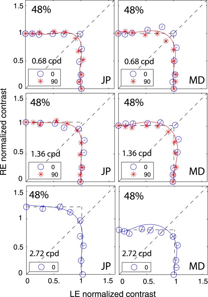
Figure 8 shows equal perceived binocular contrast contours (physical contrast 48%) drawn across different interocular contrast ratios δ for gratings of 0.68, 1.36, and 2.72 cpd when stimulus duration was 1 s and interocular phase difference was either 0° (blue circles) or 90° out of phase (red stars). The contrast of the two eyes' sine waves was normalized by the standard contrast. The contours are almost symmetrical across the δ = 1 line (dashed 45° black line) at 0.68 and 1.36 cpd, and they are very similar when the interocular phase difference varies from 0° to 90°. The DSKL model (Model 3c) with an added motor/sensory fusion mechanism with the same model parameters used for fitting the phase data (Experiment 1) accurately predicts this phase-independence of binocular contrast combination at high contrast levels (solid curves). The horizontal and vertical dashed lines are predictions from the winner-take-all model; the stimulus in the eye with stronger contrast wins the competition to give the contrast percept of the binocular-combined gratings while completely ignoring the other eye's stimulus. Interestingly, this winner-take-all model also provides a reasonable fit to the data, reflecting binocular perceived contrast being nearly constant at all interocular contrast ratios.

Figure 8.

Results of Experiment 2 at different spatial frequencies when the standard contrast was 48% and the stimulus duration was 1 s. Binocular equal-contrast contours by comparing the contrast of binocular-combined sine-wave grating with the contrast of standard grating that was always in LE when RE/LE contrast ratio was 0, 0.125, 0.25, 0.5, 0.707, 1, 1.414, 2, 4, 8, or ∞. The contrast of the two eyes' sine waves was normalized by the standard contrast. The sine waves presented to the two eyes were either 0° (blue circles) or 90° out of phase (red stars). The solid curve is the best fit from Model 3c with the same model parameters for fitting data from Experiment 1.

Phase-dependence of contrast combination

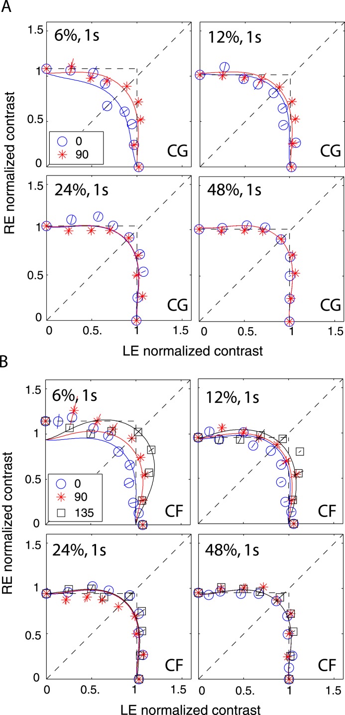
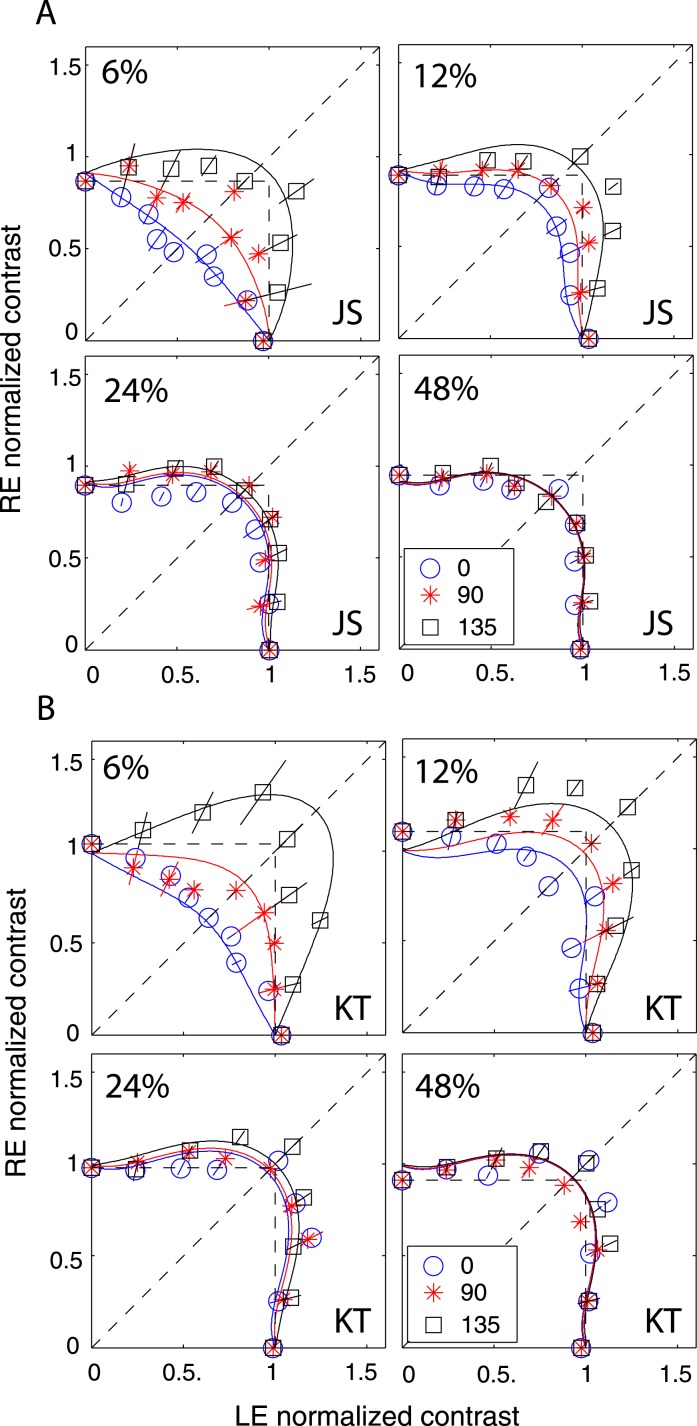
Although Figure 8 shows phase-independence of contrast combination at a high contrast level (48%) and a long stimulus duration (1 s), the model with a motor/sensory fusion mechanism predicts that the contrast combination is phase-dependent at a low contrast level when disparity energy is close to threshold and becomes more and more phase-independent as contrast (and therefore disparity energy) increases. To test this prediction, we performed Experiment 2 for two observers with the standard grating varying in contrast from low (6%) to high (48%) with a one second stimulus duration (Figure 9) and for another two observers with a stimulus duration too brief for vergence eye movements (117 ms—Figure 10). The spatial frequency was fixed at 0.68 cpd. At high contrast (48%), similar to Figure 8, the binocular-perceived contrast was almost independent of interocular phase difference for both long (1 s) and short (117 ms) stimulus durations. However, at low contrast (6%), the phase dependence of contrast combination could be observed. At the short duration (117 ms, Figure 10), the phase dependence was very obvious at 6% contrast, and the data became more phase-independent as the standard contrast increased to 48%, as predicted by DSKL model (solid curves).

Figure 9.

Results of Experiment 2 at different contrast levels when stimulus spatial frequency was 0.68 cpd and stimulus duration was 1 s. The contrast of the two eyes' sine waves was normalized by the standard contrast. The sine waves presented to the two eyes were 0° (blue circles), 90° (red stars), or 135° (black squares) out of phase, and RE/LE contrast ratio was 0, 0.25, 0.5, 0.707, 1, 1.414, 2, 4, or ∞. The solid curve is the best fit from DSKL model with the same model parameters for fitting data from Experiment 1.

Figure 10.

Results of Experiment 2 at different contrast levels when stimulus spatial frequency was 0.68 cpd and stimulus duration was 117 ms. The contrast of the two eyes' sine waves was normalized by the standard contrast. The sine waves presented to the two eyes were either 0° (blue circles), 90° (red stars), or 135° (black squares) out of phase, and RE/LE contrast ratio was 0, 0.25, 0.5, 0.707, 1, 1.414, 2, 4, or ∞. The solid curve is the best fit from DSKL model with the same model parameters for fitting data from Experiment 1.

Model fitting

Comparison of models

We tested five models of binocular combination of both phase and contrast. Let N_p be the number of model parameters and N_data be the number of observed data points. We have the number of degrees of freedom ν = N_data − N_p, and the reduced chi-square is given by ${\chi }_{\nu }^2$ = χ²/ν. If Model A is nested within Model B, the F test that tests whether Model B significantly improves data fitting is given by

which compares the variance between Models A and B with the variance inside Model B and has an F distribution with [ν(a) – ν(b), ν(b)] degrees of freedom. When the F-value is large enough, Model A can be rejected at a small false-rejection probability p(F).

Table 1 shows chi-square values for model fitting and statistical comparisons of Models 1, 2, 3a, 3b, and 3c (M1–3c), in which a previous model is nested within its successor. The comparison of two neighboring models was made through an F test with the F-value given in the row of the second model. With three steps of modification (Models 3a–c) of the Ding-Sperling model (Model 2), Models 3a and 3c achieved significant improvement in data fitting; the previous model could be rejected with a very small (<0.001) probability of false rejection. However, without gain control of the gain enhancement (Model 3c), the gain enhancement itself in Model 3b failed to further improve the data fitting in three observers.

Table 1.

Statistics of model fitting and model comparison. A previous model is nested within its following model. Notes: Np: the number of parameters; v: the number of the degrees of freedom; M1–3c: Model 1–3c.

	Np	JP				MD				CG				CF				JS				KT
		χ2/ν	${\chi }_{\nu }^2$	F	p(F)	χ2/ν	${\chi }_{\nu }^2$	F	p(F)	χ2/ν	${\chi }_{\nu }^2$	F	p(F)	χ2/ν	${\chi }_{\nu }^2$	F	p(F)	χ2/ν	${\chi }_{\nu }^2$	F	p(F)	χ2/ν	${\chi }_{\nu }^2$	F	p(F)
M1	3	960/164	5.85			1721/177	9.72			884/104	8.49			1811/155	11.7			1850/131	14.1			1820/131	13.9
M2	4	949/161	5.89	0.6	1	1573/174	9.04	5.5	<0.001	439/103	4.26	105	<0.001	1250/154	8.1	70	<0.001	511/130	3.93	341	<0.001	663/130	5.1	227	<0.001
M3a	5	521/160	3.25	132	<0.001	1177/173	6.8	58	<0.001	168/102	1.65	164	<0.001	620/153	4.05	155	<0.001	349/128	2.72	30	<0.001	596/129	4.62	15	<0.001
M3b	7	445/156	2.85	6.6	<0.001	1041/169	6.16	5.5	<0.001	168/100	1.68	0	1	617/151	4.09	0.4	1	349/127	2.74	0	1	482/127	3.79	15	<0.001
M3c	8	393/155	2.53	21	<0.001	740/168	4.4	69	<0.001	151/99	1.53	11	<0.001	530/150	3.53	24.8	<0.001	228/126	1.81	66	<0.001	453/126	3.59	8	<0.001

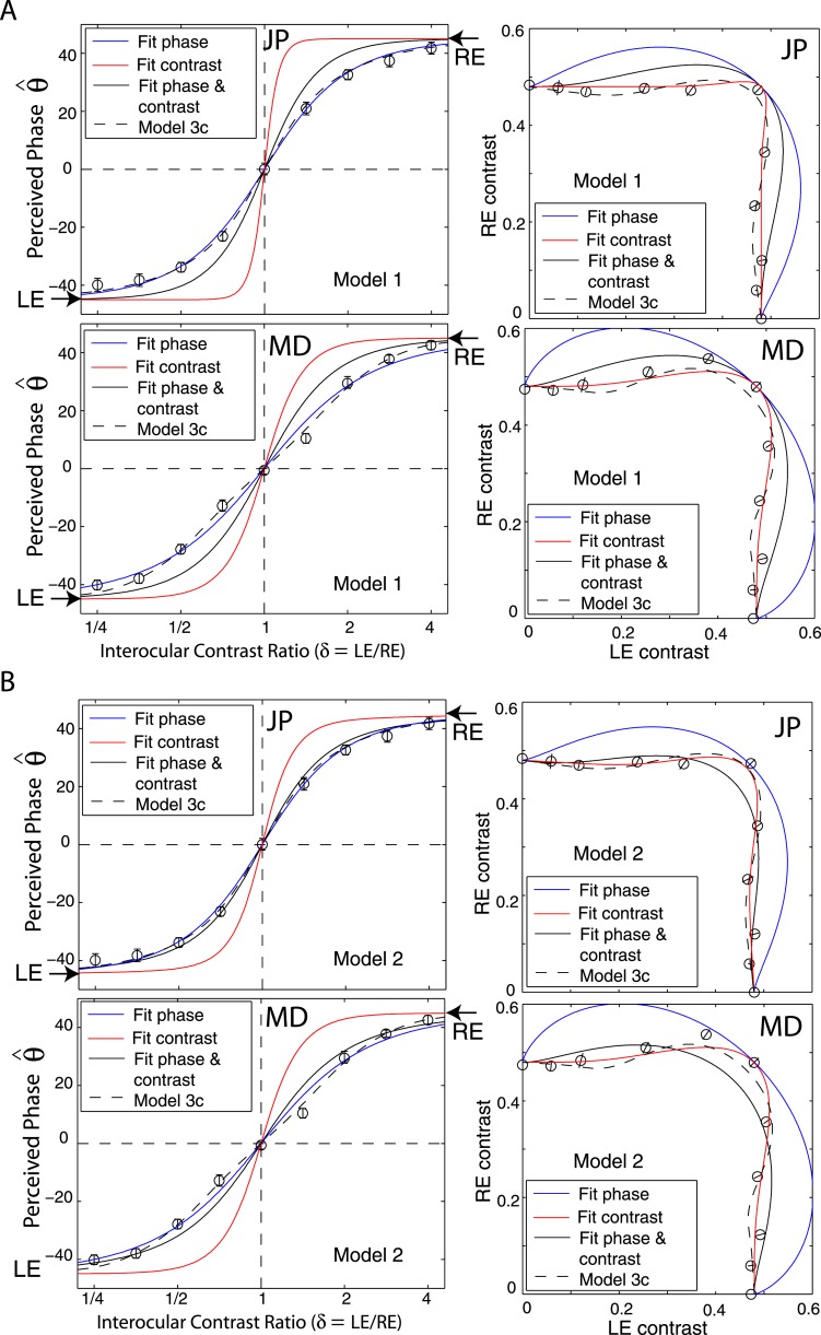
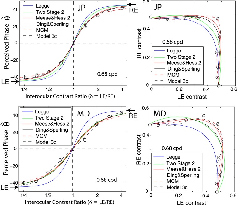
In order to get a better understanding of why the Ding-Sperling model failed in fitting both phase and contrast data simultaneously, we first fit the model only to the phase data and used the best fitting model parameters to predict the contrast contour. We then fit the model only to the contrast data and predicted the perceived phase shift. To be clear in visualization, we reduced the data set to include only one spatial frequency (0.68 cpd) and base contrast (48%) for model fitting for two observers JP and MD. Because both eyes had similar contrast sensitivity for our observers at 0.68 cpd, the attenuation (μ) was assumed to be one; Model 1 has one parameter (γ) and Model 2 has two parameters (γ and g_c). The top-left panels in Figures 11A and B demonstrate that fitting Model 1 only to the phase data (blue curve) provides a reasonable fit, but its prediction of the contrast contour (blue curve in top-right) is far removed from the data. The predicted contrast contour shows a strong Fechner's paradox, i.e., inhibition of one eye's monocular contrast perception by a small input in the other eye; however, the observed data shows a winner-take-all phenomenon, with no apparent inhibition from the other eye's image (which has smaller contrast). When fitting Model 1 only to the contrast data (red curve in top-right of Figures 11A and B), the fit again seems reasonable, but with different model parameters from fitting the phase only. However, the predicted phase (red curve in top-left) switches from one eye to the other much more rapidly than shown by the data. Although the same model can fit either phase or contrast data separately, the best fitting model parameters are not consistent, large γ values (12.5 for JP; 3.9 for MD) for contrast fitting and small γ values (1.3 for JP and 0.8 for MD) for phase fitting. When fitting Model 1 to the two data sets simultaneously (the black curves), with a trade-off γ value (2.6 ± 0.5 for JP and 1.7 ± 0.3 for MD), the fits to both data sets are poor. When fitting Model 2 to either phase or contrast data separately, similar to fitting Model 1, the best fitting model parameters are not consistent although each separate fit appears reasonable. However, when fitting Model 2 to both phase and contrast data, the goodness of fit was improved in comparison to Model 1.

Figure 11.

Fitting a model only to phase (blue solid curve), only to contrast (red solid curve), or to both phase and contrast (black solid curve). The best fitting to both phase and contrast of the full model, Model 3c, is also given (black dashed curve).

By selecting a suitable gain-control threshold g_c (0.22 ± 0.02 for JP; and 0.14 ± 0.03 for MD), the monocular contrast perception in one eye would not be suppressed by the other eye's small input if its contrast is smaller than g_c, resulting in a better fit to the data. However, when g_c is not zero (as supposed in Model 1) or small enough, the predicted binocular-combined contrast when both eyes are presented with identical images (contrast ratio = one) would not be the same as the contrast in monocular view; the prediction falls far from the observed data, as shown in the bottom-left panels of Figures 11A and 11B. To solve this problem, we introduced interocular gain enhancement (Model 3c, dashed black curves in Figure 11). By selecting suitable gain-control and gain-enhancement thresholds, g_c and g_e, and suitable α, β, and γ values, interocular gain control and gain enhancement maintain a reasonable balance in binocular vision, achieving constant contrast perception (apparent winner-take-all phenomenon) and smoothly shifting phase perception (with a reasonable exponent parameter) when interocular contrast ratio varies. To better understand how Model 3c works this way, we simulated the model using model parameters fitted to both phase and contrast data.

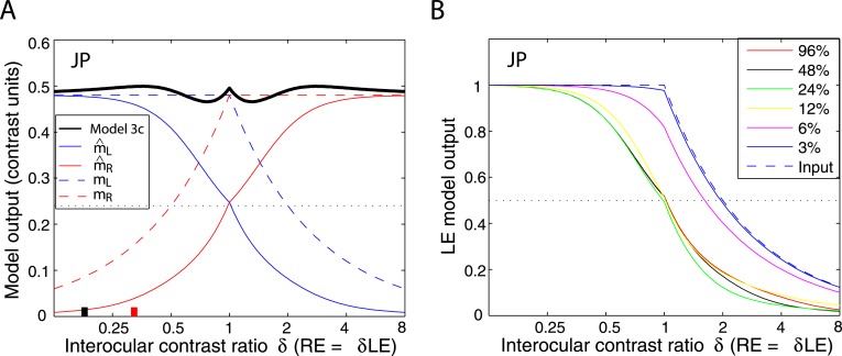
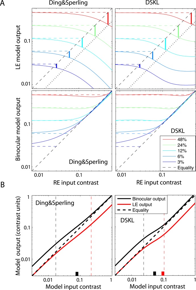
Figure 12A shows the perceived contrast predicted from Model 3c (solid black curve) as a function of interocular contrast ratio when the base contrast (the maximum of the two eyes' contrast) was 48%. Monocular inputs (dashed colored curves) and outputs (solid colored curves) of the model are also shown as functions of contrast ratio. Model 3c maintains constant contrast perception (solid black curve) through balancing gain control (its threshold is indicated by a short black vertical bar) and gain enhancement (its threshold is indicated by a short red vertical bar) to cancel the increase in the RE's apparent contrast (red solid curve) by decreasing the LE's apparent contrast (blue solid curve); both the LE's and RE's apparent contrast vary smoothly (exponent γ value is reasonable for binocular phase combination) when the contrast ratio RE/LE increases. Note that this is quite different from winner-take-all models (e.g., the Legge model with an infinite exponent), which fail to predict the smooth phase shift in binocular phase combination. However, at low base contrast, Model 3c predicts binocular linear summation. Figure 12B shows the LE's apparent contrast predicted from Model 3c when the base contrast decreases from 96% to 3%. When the base contrast is above 12%, the normalized LE apparent contrast curves are almost overlaid. When the base contrast decreases to 6% and 3%, the LE's apparent contrast curves shift toward the LE's input curve (dashed blue curve) and is almost identical to the input curve at 3% base contrast, because the system becomes more linear at lower base contrast.

Figure 12.

Simulation of the DSKL model (Model 3c) for observer JP. (A) Binocular combined contrast (solid black curve) predicted from the DSKL model when interocular contrast ratio varies and the base contrast, the maximum of two eyes' contrast, is 48% (see Figure 2). The two eyes' input contrast (dashed blue curve: left eye; dashed red curve: right eye) and their model outputs (apparent contrast) (solid blue curve: left eye; solid red curve: right eye) predicted from Model 3c after interocular interaction are also shown. The black vertical short bar shows the ratio at which the RE's contrast reaches the gain-control threshold g_c, and the red vertical short bar shows the ratio at which the RE's contrast reaches the gain-enhancement threshold g_e in Model 3c. The horizontal dotted black line indicates half of the base contrast (0.24). (B) The left eye's model output (apparent contrast) (normalized by base contrast) predicted from the DSKL model when the base contrast is 96% (red), 48% (black), 24% (green), 12% (yellow), 6% (magenta), or 3% (blue) and interocular contrast ratio, RE/LE, varies from 0.125 to 8. Left eye's input contrast is also shown (blue dashed line).

Table 2 shows the parameters of Model 3c that best fit both phase (Figures 6–7) and contrast (Figures 8–10) data sets in binocular combination. For each spatial frequency (f_s) channel, there are seven model parameters for binocular summation but four of them are shared across different frequency channels. For the disparity energy calculation in the motor/sensory fusion mechanism, there are two model parameters. Therefore, for observers CG, CF, JS, and KT who were tested only at 0.68 cpd, there are nine parameters in total. For observers JP and MD who were tested at three spatial frequencies, there were 13 parameters in total; parameters for disparity energy were fixed (g_f = 0.038 averaged from observers CG and CF and γ_f = 1).

Table 2.

Parameters of Model 3c.

Stimulus duration	fs (cpd)	μ	gc	α	γ	ge/gc	β	γ*	gf	γf
JP
1000 ms	0.68	1.0	0.013			7.87
		± 0.01	± 0.005			± 2.91
	1.36	0.93	0.027	0.84	2.35	9.72	0.12	1.48	0.038	1
		± 0.013	± 0.007	± 0.05	± 0.15	± 4.2	± 0.043	± 0.28
	2.72	0.80	0.042			9.39
		± 0.03	± 0.008			± 3.79
MD
1000 ms	0.68	0.97	0.012			4.70
		± 0.014	± 0.005			± 1.54
	1.36	0.98	0.021	0.47	2.30	4.94	0.10	1.98	0.038	1
		± 0.01	± 0.007	± 0.09	0.22	± 1.64	± 0.04	± 0.29
	2.72	1.28	0.03			4.79
		± 0.02	± 0.012			± 1.53
CG
1000 ms	0.68	0.97	0.029	1.01	1.94	3.16	0.77	1.64	0.040	0.59
		± 0.01	± 0.02	± 0.07	± 0.11	± 2.73	± 0.65	±0.19	± 0.01	± 0.29
CF
1000 ms	0.68	1.06	0.007	0.85	1.71	4.43	0.38	1.61	0.035	0.41
		± 0.01	± 0.02	± 0.08	± 0.10	± 5.17	± 0.45	±0.12	± 0.01	± 0.11
KT
117 ms	0.68	1.01	0.053	0.58	2.12	1.83	0.52	2.21	0.071	0.62
		± 0.01	± 0.005	± 0.09	± 0.20	± 0.23	± 0.17	±0.16	± 0.01	± 0.16
JS
117 ms	0.68	1.10	0.053	0.50	2.05	1.57	0.46	2.08	0.066	0.54
		± 0.01	± 0.01	± 0.08	± 0.20	± 0.16	± 0.12	±0.14	± 0.01	± 0.09

Discussion

Winner-take-all and constant contrast perception under normal viewing conditions

As noted by Blake and Fox (1973), “The simple experiment of closing one eye does not result in any dramatic change in the appearance of the visual world.” Indeed, under normal viewing conditions (high contrast and long duration), our contrast combination results are apparently consistent with a winner-take-all model (horizontal and vertical dashed lines in Figures 8–9), reflecting constant contrast perception in normal binocular vision at all interocular contrast ratios. However, this apparent winner-take-all behavior is not the outcome of a winner-take-all mechanism because the apparent switch behavior is not observed in the perceived phase of a cyclopean sine wave, which shifts continuously from left to right eye when the contrast ratio RE/LE increases from zero to infinity (Figure 6). As shown in Figure 12A, this winner-take-all phenomenon under normal viewing conditions is the approximate outcome of more complex interocular interactions, including both gain controls and gain enhancements as described in the DSKL model.

The nearly constant contrast perception under normal viewing conditions places a strong constraint on modeling binocular combination. Our model fitting shows that the DSKL model (Model 3c), which maintains the balance between interocular suppression and enhancement, successfully predicts both the winner-take-all feature (Figures 8–9) in contrast combination under normal viewing conditions and the smooth phase shift in phase combination (Figures 6–7), improving model fitting significantly compared with Model 2.

Through balancing mutual interocular suppression and enhancement, under normal viewing conditions, the normal visual system achieves constant binocular contrast perception at all interocular contrast ratios, which extends our everyday experience that the world looks the same whether one eye is closed or both eyes remain opened (Ding & Sperling, 2006), while shifting visual direction smoothly from one eye to the other eye depending on the interocular contrast ratio. More interestingly, even observers with abnormal binocular vision achieve constant contrast perception, although not perfect for some individuals, through balancing interocular inhibition and enhancement; the contrast loss in the nondominant eye is compensated for by the contrast gain in the dominant eye (see figure 16 in the following article, Ding, Klein, & Levi, 2013).

Contrast-dependence of the linearity of binocular combination

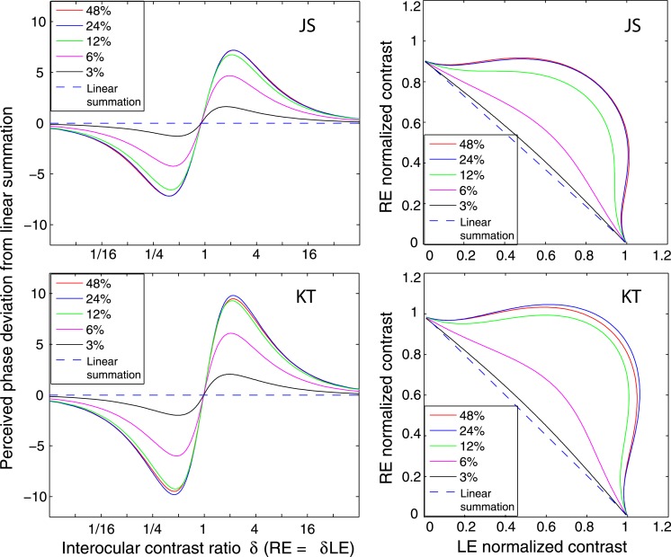
Ding and Sperling (2007) have previously reported the linear summation of binocular phase combination at low contrast energy (at low contrast and short duration), and when the contrast energy increased, the combination became more and more nonlinear. In this study, we confirmed this contrast-dependence of the linearity of binocular combination in binocular contrast combination (Figure 10). Figure 13 demonstrates the simulation of perceived phase (left column, phase deviation from linear summation is shown) and contrast (right column) predicted from Model 3c using fitted model parameters for two observers at a duration too brief for vergence eye movements (117 ms). When base contrast increased from 0% to 48%, binocular combination became systematically more nonlinear in both phase and contrast perception. However, at low contrasts near detection threshold, the matching task was more challenging, especially for phase perception, and we were unable to collect useful phase data at 6% and contrast data at 3%. Interestingly, Fechner's paradox, which was observed by Legge and Rubin (1981) at low contrast and short stimulus duration, was not evident in the present study for any of our experimental conditions for all normal observers. However, Fechner's paradox was evident for observers with asymmetric interocular suppression (see the following article). Figure 12B demonstrates that the shape of the monocular output of the model depends on base contrast; at 3% base contrast, the output is almost identical to the input.

Figure 13.

Simulation results of Model 3c when base contrast varies from 0% to 48% at stimulus duration of 117 ms. To better illustrate the linearity of phase perception, the phase deviation from linear summation is plotted as a function of contrast ratios when the base contrast is 0% (dashed line), 3% (black), 6% (magenta), 12% (green), 24% (blue), or 48% (red).

Comparison with other models

Several models have been proposed to account for binocular combination. Typically, one model was proposed to explain data collected from one specific experiment. Comparison among models in data fitting was seldom done (Blake & Wilson, 2011). Here we compare several influential models deduced from contrast matching or contrast discrimination experiments (Legge, 1984b; Meese et al., 2006; Meese & Hess, 2004; Moradi & Heeger, 2009) with the models proposed in this article and the MCM, recently proposed by Huang et al. (2010). Typically, these contrast-deduced models included nonlinear operators for binocular contrast perception. In order to account for phase data without nonlinear phase distortion, we assumed that the operations in these models only apply to contrast, and the phase remains unchanged.

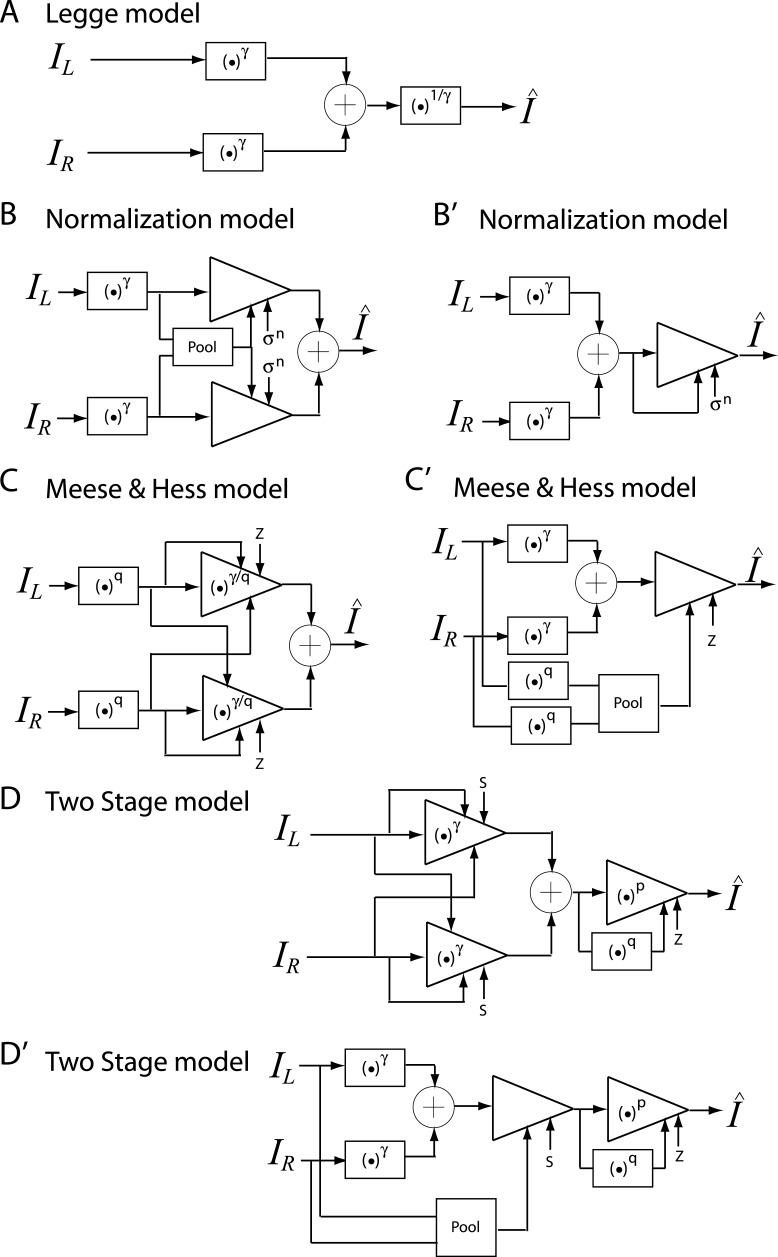
Figure 14 shows the schematic diagrams of those contrast-deduced models. Let δ = m_R/m_L be interocular contrast ratio, from the Appendix, the perceived phase and contrast from the Legge model (Figure 14A) are given by

and

respectively. When γ = 1, the Legge model is identical to the linear summation model; when γ > 1, the model predicts that the eye with higher contrast would have more weight in binocular combination than would be predicted by the linear summation; when γ = ∞, the model is identical to the winner-take-all model, predicting the perceived phase switching from one eye to the other at δ = 1 and the perceived contrast is the higher contrast of the two eyes.

Figure 14.

Model comparison. (A)–(D) Models originally deduced from contrast experiments were modified to account for both phase and contrast binocular combination by assuming that all operations only act on contrast and have no effect on the phase.

Figure 14B shows the contrast normalization model proposed by Moradi and Heeger (2009) to explain their fMRI data in binocular combination. The contrast is first extracted from both eyes and pooled together and then the pooled contrast exerts gain control to the two eyes separately before binocular combination. From the Appendix, the perceived phase from the normalization model is also given by Equation 12, and the perceived contrast is given by

However, as shown in the Appendix, the formula for fitting data from contrast matching tasks deduced from the normalization model is identical to that deduced from the Legge model. Actually, it becomes obvious that the normalization model is equivalent to the Legge model in binocular combination if we redraw the normalization model in Figure 14B′; the two eye's inputs are first combined and then the combined contrast energy exerts gain control to the combined signal as shown in the second equation of Equation 14. Because the calculations after binocular combination have no effect on the perceived phase and the contrast matching, the normalization model performs the same way as the Legge model in binocular combination, making model parameter σ insignificant in data fitting. In other words, the gain control in the normalization model could be considered as a binocular contrast gain control, which accounts for the contrast transfer function in monocular and binocular vision. Therefore, its behavior in fitting our data is identical to the Legge model; its gain-control path plays no role in binocular combination. However, if different weights are assumed for monocular and interocular gain controls in the normalization model, the model would contain both monocular and interocular mechanisms. From this modified normalization model, the perceived contrast is given by

where w is the relative weight for interocular gain control when the weight for monocular gain control is assumed to be one. The perceived phase is given by Equation A18 with apparent contrast ratio calculated by Equation A49.

In contrast, the gain control in the Ding-Sperling model (Model 2) could be considered as an interocular contrast gain control without any monocular mechanism. When contrast m is presented in one eye only, the perceived contrast predicted from the Ding-Sperling model or any other model in this study always equals to m, i.e., mˆ = m when one eye is closed. Without adding monocular mechanisms, it is impossible to account for contrast discrimination data from our models.

The Meese-Hess model (Figure 14C) looks similar to the normalization model except that the signal and control paths take different power operations. Again, the perceived phase is also given by Equation 12, and the model could be redrawn in Figure 14C′. The perceived contrast is given by

which could also be considered as a binocular contrast gain control without interocular mechanisms. When fitting the phase data only, model parameters in the control path could have any value, having no effect on the fitting results. When fitting both phase and contrast data, the model should be reduced to a two-parameter model, either with a fixed gain-control constant Z, which might be determined from contrast transfer function or with the power in the control path q depending on the power in the signal path γ. We reduced the model by letting q = γ − 1, and we have

To include interocular mechanisms in the model, different weights should be assumed for monocular and interocular gain controls. We have

The perceived phase is given by Equation A18 with apparent contrast ratio calculated by

The two-stage model (Figure 14D) was proposed by the same group as the Meese-Hess model to extend it to account for the finding of less nonlinearity at lower contrast, using gain control with an exponent near-to-one in the first stage before binocular combination and to account for high nonlinearity at higher contrast using the gain control in a second stage after binocular combination. However, like the Meese-Hess model, the gain control in the first stage could be considered as a binocular contrast gain control after the binocular combination as shown in Figure 14D′. The parameters in the control path have no effect on the prediction of perceived phase, which is also given by Equation 12 deduced from the Legge model. When fitting both phase and contrast data, the model has to be reduced to a two-parameter model with only the first stage; the parameters in the second stage couldn't be determined from our data. From this reduced model, the perceived contrast is given by

Again, to include interocular mechanism, different weights are assumed for monocular and interocular gain controls. We have

The perceived phase is given by Equation A18 with apparent contrast ratio calculated by

Without the asymmetry assumption of monocular and interocular gain controls, all these models deduced from contrast combination have no effective interocular mechanisms. The contrast gain control in the normalization, Meese-Hess, or two-stage model is actually a binocular gain control because both eyes gains increase or decrease in exactly the same way no matter which eye's contrast increases or decreases. The perceived phase is only determined by the signal path of the model; all four models give the same prediction of the perceived phase given by Equation 12. On the other side, in the Ding-Sperling model, increasing the left eye's contrast would decrease the right eye's gain but, at the same time, it would increase the left eye's gain through suppressing the gain control from the right eye, and vice versa.

In the following, we compare the models we proposed in this article and the MCM proposed by Huang et al. (2010) with those models deduced from binocular contrast combination of two in-phase sine waves for fitting our data. To make things simple and to be clear in visualization, we only fit each model to a reduced data set when two eyes' sine waves have the spatial frequency of 0.68 cpd and they are in phase for contrast combination. We assumed μ = 1 for all our five models and γ* = γ for Models 3b and 3c.

We used the Akaike information criterion (AIC), a measure of the relative goodness of fit of a statistical model developed by Akaike (1974), to compare different models. Let N_p be the number of model parameters and L_Max hais the maximized value of the likelihood function for the estimated model; AIC is defined as AIC = 2N_p – 2 ln L_Max. Assuming that the errors are normally distributed and independent, after ignoring the constant term, AIC is given by AIC = χ² + 2N_p.

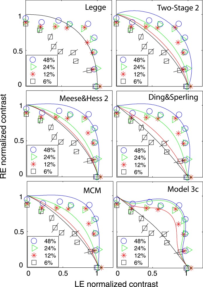
Table 3 shows the statistical results of fitting twelve models, five proposed in this article and seven from the literature, to the data. Both the Legge model (Equations 12 and 13, Figure 14A) and Model 1 (Equation 3) have only one parameter. They give similar phase predictions (Equation A18 vs. Equation A40) but different contrast predictions (Equation A20 vs. Equation A41). At high base contrast (48%, observers JP and MD), the AIC scores of the fits are much reduced for Model 1 compared to the Legge model, indicating a significantly better fit. However, when the base contrast was tested at several levels from 6% to 48% (observers CG, CF, JS, and KT), the AIC scores of the fits are much reduced for the Legge model. Because Model 1 is a reduced gain-control model with an assumption of zero gain-control threshold, i.e., g_c = 0, giving the same prediction at all contrast levels, it would give a better fit only at high contrast than the Legge model. When fitting a range of contrast levels, the data was more linear at lower contrast levels and became more nonlinear as contrast increased. Model 1 failed to pick up the linear feature at low contrast, making it worse in data fitting than the Legge model. For the purpose of fitting our data, the normalization model (Figure 14B) is essentially identical to the Legge model, and both models have the same chi-squared statistics.

Table 3.

Statistics of chi-squared and fitted exponent values for model fitting to our reduced data set. Notes: Np: the number of parameters; v: the number of the degrees of freedom; AIC: Akaike information criterion; γ: fitted exponent values.

Model	Np	JP				MD				CG				CF				JS				KT
		χ2/ν	${\chi }_{\nu }^2$	AIC	γ	χ2/ν	${\chi }_{\nu }^2$	AIC	γ	χ2/ν	${\chi }_{\nu }^2$	AIC	γ	χ2/ν	${\chi }_{\nu }^2$	AIC	γ	χ2/ν	${\chi }_{\nu }^2$	AIC	γ	χ2/ν	${\chi }_{\nu }^2$	AIC	γ
Legge	1	222/19	11.7	224	3.59	603/19	31.8	605	3.45	406/71	5.71	408	3	834/86	9.7	836	2.62	693/62	11.2	695	2.32	900/62	14.5	902	2.27
Model 1	1	182/19	9.57	184	2.6	274/19	14.4	276	1.73	700/71	9.87	702	2.25	1826/86	21.2	1828	2.06	1812/62	29.2	1814	3.14	1524/62	24.6	1526	1.68
Two-stage	2	166/18	9.24	170	3.02	187/18	10.4	191	2.07	197/70	2.82	201	2.34	511/85	6.05	518	2.14	409/61	6.71	413	1.45	447/61	7.33	451	1.65
Meese-Hess	2	107/18	5.94	111	2.96	166/18	9.21	170	2.27	198/70	2.83	202	2.34	519/85	6.11	523	2.11	483/61	7.92	487	1.85	491/61	8.04	495	1.83
Model 2	2	41/18	2.26	45	2.18	118/18	6.57	122	1.44	309/70	4.42	313	1.79	1045/85	12.3	1049	1.09	259/61	4.24	263	1.33	356/61	5.84	360	1.25
Modified two-stage	3	166/17	9.74	172	2.95	162/17	9.52	168	1.70	187/69	2.71	193	2.41	465/84	5.54	471	2.32	322/60	5.36	328	1.24	440/60	7.33	446	1.63
Modified normalization	3	50/17	2.95	56	2.35	60/17	3.53	66	1.85	261/69	3.78	267	2.53	618/84	7.35	624	2.28	270/60	4.5	276	1.36	454/60	7.56	460	1.84
MCM	3	10.5/17	0.62	17	3.12	63/17	3.73	69	2.02	159/69	2.30	165	1.46	494/84	5.87	500	1.20	257/60	4.28	263	1.46	356/60	5.93	362	1.16
					1.34				1.49				0.84				0.79				1.21				0.98
Model 3a	3	16/17	0.95	22	2.22	59/17	3.48	65	1.6	140/69	2.03	146	1.76	427/84	5.08	433	1.5	249/60	4.15	255	1.48	331/60	5.51	337	1.34
Modified	4	50/16	3.15	58	2.32	60/16	3.75	68	1.85	149/68	2.19	157	2.25	431/83	5.2	439	2.53	271/59	4.59	279	1.37	384/59	6.51	392	1.70
Meese-Hess					2.32				1.85				2.2				1.98				1.37				1.70
Model 3b	4	16/16	1.01	24	2.22	59/16	3.7	67	1.61	140/68	2.06	148	1.59	440/83	5.31	448	1.38	250/59	4.24	258	1.79	347/59	5.89	355	1.2
Model 3c	5	13/15	0.86	23	3.37	28/15	1.84	38	4.87	138/67	2.06	148	1.71	378/82	4.61	388	1.75	141/58	2.42	151	1.88	253/58	4.37	263	2.73

Next, we compared two-parameter models, the Meese-Hess model (Figure 14C), the two-stage model (Figure 14D), and Model 2 (the original Ding-Sperling model, Figure 4B). Model 2 provided a much better fit to the data than the other two-parameter models for observers JP, MD, JS, and KT. However, for observers CF and CG, both the two-stage and Meese-Hess models provide a much better fit than Model 2. Adding an additional parameter to make the gain controls of the two layers asymmetric, Model 3a provided significantly improved fits over Model 2. Also, the modified normalization model and the modified Meese-Hess model with asymmetric monocular and interocular gain controls significantly improved data fitting over the original models (see statistics of the Legge model for the original normalization model). However, the modified two-stage model failed to improve data fits for observers JP and KT although it significantly improved data fitting for four other observers.

Interestingly, by adding an extra exponent parameter only for contrast perception, the MCM significantly improved the data fits over Model 2 for four observers who collected data at a long stimulus duration (1 s), but it failed to improve the fits for observers JS and KT who collected data at a short stimulus duration (117 ms). Model 3a seems adequate for fitting this reduced dataset for observers JP, MD, and CG; the reduced chi square for observer JP is less than one, indicating a very good fit. Adding enhancement (Model 3b) did not further improve the fitting performance for this small data set; the chi-square is the same as in Model 3a for three observers. The addition of enhancement and gain control of the enhancement (Model 3c—the DSKL model) further improved the fit for observers JP and MD but not for observer CG. For fitting the full data set (Table 1) or for fitting the data of observers with abnormal binocular visual experience (see the following article), the modifications in Models 3a and 3c significantly improved data fitting.

Figure 15 shows fitting results from these models to both phase and contrast data for observers JP and MD at spatial frequency of 0.68 c/°, base contrast of 48%, and stimulus duration of 1 s. Fitting either the phase or contrast data separately, each of these models provides a reasonable fit (data not shown, see discussion of Figure 11), but with different fitted exponent gamma values for the Legge, modified two-stage, modified Meese-Hess, and Ding-Sperling models. By adding an additional exponent parameter to the Ding-Sperling model only for the contrast perception, the MCM successfully predicts both phase and contrast data (red dashed curve in Figure 15) under normal viewing conditions (high stimulus contrast and long stimulus duration), consistent with a previous study (Huang et al., 2010). However, MCM is based on the assumption of phase-independent binocular contrast combination that was shown not to be valid at low contrasts (Baker et al., 2012) and therefore failed to pick up the phase-dependence shown in Figures 9 and 10. By adding interocular enhancement to the Ding-Sperling model, the DSKL model (Model 3c—black dashed curve in Figure 15) also provides a good fit to both phase and contrast data. The phase data fits are very similar among these models for normal vision because they have the same or similar apparent interocular contrast ratio. However, the contrast data fits are quite different; with the constraints of perceived phase, the Legge model (blue curve) fails to account for the data of binocular combined contrast.

Figure 15.

Model predictions from Legge, modified two-stage (Two Stage 2), modified Meese & Hess (Meese & Hess 2), Ding & Sperling, MCM, and DSKL (Model 3c). Model fits to both phase (left) and contrast (right) data for observers JP and MD at 48% of base contrast, 1 s of stimulus duration, and 0.68 cpd. The interocular phase difference was fixed at 90° for phase perception, but the two eyes sine waves were in phase for contrast perception.

Figure 16 compares contrast fitting results of these models when fitting them to both phase and contrast data for observer JS at 117 ms stimulus duration and 6%–48% of base contrast. Phase fittings (not shown) were very similar to those in Figure 15. When base contrast varies from 6% to 48%, the contrast combination data demonstrate nearly linear summation at 6% base contrast and highly nonlinear summation at 48%; the nonlinearity of the contrast contours increases when the base contrast increases. However, with only one model parameter, the Legge model failed to pick up this feature; the fitted curves are overlaid for all base contrasts. All other models correctly pick up this feature. However, for the modified two-stage model (Two-Stage 2) and modified Meese-Hess model (Meese & Hess 2), the model is not sufficiently nonlinear at high contrast levels to fit the nonlinear contour data at 48% while at low contrast it is not linear enough to fit the linear summation at 6%. Although the two models include a constant term in their gain-control path, giving no gain controls at low contrast, their signal paths also include nonlinear terms in order to account for nonlinear features at high contrast which results in their failure to predict the linear summation contour at low contrast. The Ding-Sperling model, which has only linear operators in its signal path, correctly predicts the binocular linear summation at low contrasts when the contrast energy is lower than its gain-control threshold, therefore improving the data fit at 6%, but it still misses data points at a higher contrast. It is not sufficiently nonlinear at high contrasts to account for the data. By adding an additional exponent gamma value to the Ding-Sperling model only for contrast perception, the MCM seems somewhat limited, although it does provide a reasonable fit at high contrast levels (Figure 15). By adding interocular enhancement to the Ding-Sperling model, making it more nonlinear at high contrast while still keeping it linear at low contrast when the contrast energy is less than both gain-control and gain-enhancement thresholds, the DSKL model successfully predicts both high nonlinear contrast contour at 48% and linear contrast summation at 6%. Importantly, while there may be other ways to achieve this in observers with normal vision, the gain enhancement is necessary for fitting the highly nonlinear data of observers with abnormal binocular vision (see subsequent article, Ding, Klein, & Levi, 2013).

Figure 16.

Model predictions from Legge, modified two-stage (Two Stage 2), modified Meese & Hess (Meese & Hess 2), Ding & Sperling (Model 2), MCM, and DSKL (Model 3c). Model fits to both phase (not shown) and contrast data for observer JS at 6%–48% of base contrast, 117 ms of stimulus duration, and 0.68 cpd. The interocular phase difference was fixed at 90° for phase perception, but the two eyes sine waves were in phase for contrast perception.

Phase-dependence of binocular contrast combination

The Ding-Sperling model was originally developed to explain and predict the results of binocular phase combination experiments. An important prediction of the model was the phase dependence of binocular combination, which was confirmed experimentally (Ding & Sperling, 2006, 2007; Huang et al., 2009; Huang et al., 2011; Huang et al., 2010) (also see the following article). However, binocular contrast combination is phase independent under normal viewing conditions (high contrast and long stimulus duration) (Huang et al., 2010, 2011), but is phase dependent at low contrast (Baker et al., 2012). In order to account for their data, Huang et al. (2010, 2011) elaborated the Ding-Sperling model by adding an additional channel for contrast perception after first processing the two eyes' inputs through the Ding-Sperling model and assuming phase-independent contrast power summation in the contrast channel (MCM). Although the MCM achieves a satisfactory fit to their data under normal viewing conditions, it fails to predict the phase dependence of contrast combination at low contrasts (Baker et al., 2012), fails to predict contrast combination over a broader range of contrast levels even when the two eyes' sine waves were always in phase (see the bottom-left panel in Figure 16), and also fails to account for binocular combination in abnormal binocular vision (see the following article). One possible reason for the differences between their data and ours may be because they used the method of adjustment with viewing durations as long as 10 s.

A motor/sensory fusion mechanism

We incorporated a motor/sensory fusion mechanism into our binocular combination model to account for both phase and contrast data when interocular phase difference varied. Under normal viewing conditions, when the two eyes are presented with two images that have a small offset in position, disparity vergence (motor fusion) operates through a visual feedback control system to minimize binocular disparity with an appropriate binocular convergence or divergence. However, motor fusion may not be sufficient to eliminate the physical disparity, especially when binocular fusion locks are presented in the surround, as was the case in this study (Schor et al., 1984). Typically, physical disparity is larger than the vergence (vergence error or fixation disparity). A sensory process (sensory fusion) is needed to compensate for the remaining vergence error to align the two eyes images.

We assume that the brain performs sensory fusion through remapping of the corresponding points of the two eyes (Fogt & Jones, 1998a, 1998b; Hyson et al., 1983). The site for remapping has been proposed to be as early lateral geniculate nucleus, which has multiple layers that have different maps from the retina (Richards, 1968). In a control experiment, we measured vergence subjectively (using nonius lines) when an observer viewed 90° out-of-phase dichoptic sine waves in the same setup (with strong binocular fusion locks in the surround) as in Experiments 1 and 2. We found that for normal observers, vergence eye movement could only compensate for ≈ 10% of the physical offset of the two sine waves; the rest must be compensated by sensory fusion. Model 3c, which includes a motor/sensory fusion mechanism, is able to account for the phase dependency of binocular contrast summation (Figures 9 and 10).

Here, we simulate Model 3c (Figure 17A) using the fitted parameters for perceived contrast when the eyes' sine waves have identical contrast but with different phases (Baker et al., 2012). The simulation captures some features of the data from Baker et al. (2012). At low standard contrast (2%), their data showed linear summation when the interocular phase difference was less than 90°, and the perceived contrast was strongly dependent on interocular phase. However, when standard contrast increases, their data showed that the binocular summation became more and more independent of phase, and at 32% contrast, the perceived contrast became almost completely independent of phase, even at 180° of the phase difference. Although the simulation in Figure 17A captures most features when the phase difference is less than 135°, it fails to predict the perceived contrast at 180° out of phase when the two sine waves have identical contrast: The model gives zero output at all contrast levels while the data from Baker et al. (2012) showed no complete cancelation—actually one eye's contrast was perceived at 32% contrast. Indeed, at 180° out of phase, binocular rivalry occurs. Unlike binocular combination, in which the binocular combined sine wave is perceived, in binocular rivalry, the perceived sine wave is either the LE's or the RE's but not combined. Although we are not clear whether the binocular combination and rivalry share the same circuit or a part of the circuit for the interocular interactions, a different mechanism related to binocular rivalry should be included in a model in order to also account for the perceived contrast when the two sine waves are 180° out of phase. Baker et al. (2012) proposed a model that also includes inhibition across different phase channels to account for their binocular-contrast-combination data when interocular phase difference varied from 0° to 180°. Their model simulation provides a reasonable explanation of their data.

Although the remapping through motor/sensory fusion altered the perceived contrast dramatically, it only changed the perceived phase very slightly. Figure 17B shows a simulation of Model 3c for perceived phase before (dashed colored curves) and after (solid colored curves) motor/sensory fusion. At both low (6%, blue) and high (48%, red) contrast, the perceived phases are very close to each other at all interocular contrast ratios.

Model behaviors of the Ding-Sperling and DSKL models

To further clarify the behavior of the DSKL model (Model 3c) and to help visualize how it differs from the original Ding-Sperling model (Model 2), we simulated the contrast outputs of the two models (Figure 18). We first simulate both models keeping one eye's (LE's) input constant while varying the other eye's (RE's) contrast (Figure 18A). Both models show interocular suppression; the LE's model output (the apparent contrast) decreases from its input levels (indicated by horizontal dashed colored lines) when the RE's input increases (top panels). However, when the RE's input further increases, the two models show different behaviors: In the Ding-Sperling model, the LE's model output decreases further, while in the DSKL model, interocular gain enhancement slows the decrease of the LE's model output, and it becomes flat. The binocular outputs (the perceived contrast) of the two models are shown in the bottom panels of Figure 18A. They behave very similarly: At low contrast, the perceived contrast increases when RE's input increases, while at high contrast, the perceived contrast shows apparent winner-take-all behavior, flat when RE < LE and then following the RE's input when RE ≥ LE. However, the DSKL model provides a more accurate description of these winner-take-all phenomena than the Ding-Sperling model. Note however, the winner-take-all behavior is not an outcome of a specific winner-take-all mechanism. Rather, at high contrast, the model output of the LE decreases by about half (indicated by the vertical colored bars in the top panels of Figure 18A) of its input when the RE's input reaches the input contrast of the LE, making the binocular output (combined two halves of the input) equal the monocular input when both eyes receive identical contrast under normal viewing conditions. The DSKL model achieves this constant contrast perception over a larger range of contrasts (>12%) than that of the Ding-Sperling model (>24%).

Figure 18.

Model simulations of Ding-Sperling and DSKL models using fitted model parameters. (A) The LE's model output in contrast units (before binocular combination) (top) and the binocular model output in contrast units (bottom) are simulated when the RE's input contrast increases but the LE's input remains unchanged at 3%, 6%, 12%, 24%, or 48%. The vertical solid bars in the top panels indicate the amount decreased from the input levels (indicated by horizontal dashed lines) in the LE when the RE's input reaches the input contrast of the LE. The black dotted line indicates the decrease by a factor of two (or half) of the LE's output. (B) Model simulations of binocular (solid black) and monocular (solid red) output (contrast units) when both eyes have identical contrast inputs. The dashed black diagonal indicates the equality of the output with the input. The short black bar indicates the gain-control threshold, and the short red bar in the right panel indicates the gain-enhancement threshold. The two vertical dashed lines separate the model output into three different behaviors: (1) linear binocular summation at low contrast, apparent exponent ≈1 (for Legge model, i.e., Binocular ≈ LE + RE); (2) constant contrast perception at high contrast, apparent exponent ≈ ∞; (3) smooth transition from the linear-summation behavior to the constant-contrast behavior, changing apparent exponent from one to ∞.

In order to get a better view of this model behavior, we simulate the models when the two eyes receive identical contrast inputs (Figure 18B). The model outputs demonstrate that both DSKL and Ding-Sperling models have three distinct behaviors (separated by two vertical dashed lines): (a) linear summation (apparent exponent ≈ 1 for Legge model, i.e., Binocular ≈ LE + RE ) at low contrast; (b) constant-contrast perception at high contrast (apparent exponent ≈ ∞); (c) smooth transition from linear-summation to constant-contrast perception, changing the apparent exponent from one to ∞. However, with both interocular gain control (its threshold is indicated by a short black bar) and gain enhancement (its threshold is indicated by a short red bar), the DSKL model has a sharper transition between linear summation and constant-contrast perception, more consistent with the experimental data (bottom-right panel in Figure 16) than the Ding-Sperling model with only interocular gain control, which failed to fit the data when the input contrast varied over a broad range (middle-right panel in Figure 16). For the DSKL model (right panel in Figure 18B), when the input contrast is lower than half of the gain-control threshold (indicated by a short vertical black bar), the model shows linear behavior without any interocular interaction; the monocular model output (solid red curve) is identical to the input and the binocular model output (solid black curve) doubles the monocular input, a linear summation of the two monocular inputs. When the input contrast is higher than twice the gain-control threshold or a little bit higher than the gain-enhancement threshold, the DSKL model achieves constant contrast perception, binocular output (solid black curve) equals monocular input, through decreasing monocular output contrast (solid red curve) by factor of two.

Any model with a nonlinear operator in its signal path (with a nonlinear numerator), such as the normalization, two-stage, and Meese-Hess models that originate from a nonlinear contrast transducer, would have trouble explaining the linear behavior in binocular combination at low contrast (see Figure 16). This linear summation at low contrasts also constrains the MCM with the exponent in its additional contrast channel very close to one (≈0.98 for the bottom-left panel in Figure 16), making it no different from the original Ding-Sperling model. Although the Legge model with different apparent exponents at different contrast levels might be able to explain binocular contrast combination, it failed to explain both phase and contrast combination simultaneously (see discussion of Figures 11, 12, and 15). The DSKL model successfully explains both linear behavior at low contrast and constant-contrast perception at high contrast and provides a sharp but smooth transition between the two behaviors.

Our experiments and modeling show that binocular combination is more complex than previously thought. However, the range of binocular interactions in normal vision may not be sufficiently large to fully distinguish amongst the many extant models of binocular combination. In the subsequent article we show that observers with abnormal binocular vision may, like dichromats in color vision, place additional constraints on the models, and provide new insight into the nature of binocular interaction.

Appendix: Calculations of the perceived phase and contrast of a cyclopean sine wave from a binocular combination model

Linear summation model

Let I_L and I_R be the stimuli presented to the left and right eyes, respectively, given by

and

The perceived sine wave is supposed to be the arithmetic summation of the two eyes' sine waves, i.e., Î = I_L + I_R. Figure A1 shows vector presentations of sine waves and their arithmetic summation in the complex plane. We have

where Î₀ = 2I₀,

and

Figure A1.

Vector presentations of sine waves and their arithmetic summation in the complex plane before (black) and after (blue) motor/sensory fusion.

Remapping corresponding points through motor/sensory fusion

After remapping of the two eyes' corresponding points through motor/sensory fusion, the misaligned two eyes' sine waves shift their phases towards the perceived phase to align with each other. Figure A1 demonstrates that, after remapping, the left eye phase shifts from θ_L (black) to ${{\theta }^{\prime }}_L$ (blue), rotating an angle of the frction of the phase difference between the left eye and the cyclopean eye, and the right eye phase shifts from θ_R (black) to ${{\theta }^{\prime }}_R$(blue), rotating an angle of the fraction of the phase difference between the right eye and the cyclopean eye. We assume that the disparity energy, given by

first goes through a gain control to calculate the fraction of disparity remapping demand,

that drives motor/sensory fusion to align two eyes' images as shown in Figure 5. We have

In Equation A7, g_f is the contrast threshold at which the motor/sensory fusion becomes apparent and γ_f is the exponent value for the gain control in the motor/sensory fusion mechanism. At very low contrast, when D << $g_f^2$, no motor/sensory fusion occurs and we have ${{\theta }^{\prime }}_L$ ≈ θ_L and ${{\theta }^{\prime }}_R$ ≈ θ_R, and the perceived contrast and phase are still given by Equations A4 and A5, respectively. At very high contrast, when D >> $g_f^2$, the motor/sensory fusion results in perfect binocular alignment, i.e., ${{\theta }^{\prime }}_L$ ≈ ${{\theta }^{\prime }}_R$ ≈ θˆ, and the perceived contrast is given by ${\mathrm{mˆ}}^{\prime }$ = m_L + m_R but the perceived phase is still given by Equation A5. Generally, after motor/sensory fusion, the perceived contrast is given by

and the perceived phase is given by

Let θ_R = θ/2, θ_L = −θ/2, and m_R = δm_L, where θ = θ_R – θ_L is the phase difference between two eyes and δ = m_R/m_L is interocular contrast ratio, then the perceived contrast and phase before motor/sensory fusion are given by

After motor/sensory fusion, the perceived contrast is given by Equation A9 and the perceived phase is given by

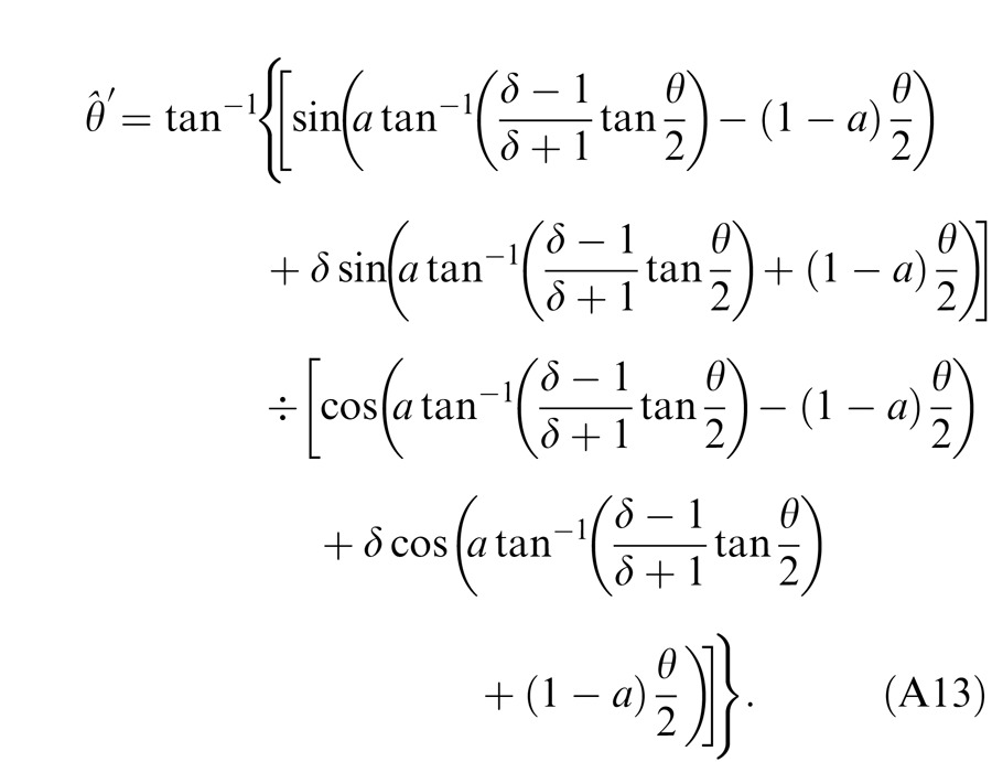When only the left eye is presented with the sine wave, i.e., m_R = 0 or δ = 0 , the perceived phase is the same as the input from the left eye, i.e., θˆ′ = θˆ = θ_L = −θ/2. When only right eye is presented with the sine wave, i.e., m_L = 0 or δ = ∞, the perceived phase is the same as the input from the right eye, i.e., θˆ′ = θˆ = θ_R = θ/2. When the two eyes are presented with the sine waves with identical contrast, i.e., m_L = m_R or δ = 1, the perceived phase is zero, i.e., θˆ′ = θˆ = 0. When interocular contrast ratio varies from zero to ∞, the perceived phase varies from the phase of the left eye sine wave, −θ/2, to the phase of the right eye sine wave, θ/2. As shown in Figure 17B, before and after motor/sensory fusion the perceived phases are very close to each other, i.e., θˆ′ ≈ θˆ, for all interocular contrast ratios at all contrast levels.

Model 1: Contrast-weighted summation model (simplified Ding-Sperling model)

After being weighted by contrast energy, the monocular signals become

and

From Equations 4 and 5, we have

Therefore the apparent interocular contrast ratio is given by

When θ_R = θ/2, θ_L = −θ/2 (the case for Experiment 1), the perceived phase of a cyclopean sine wave is given by

With the fraction of the disparity remapping demand given by

After remapping of two eyes' corresponding points through motor/sensory fusion, the perceived contrast and phase are given by

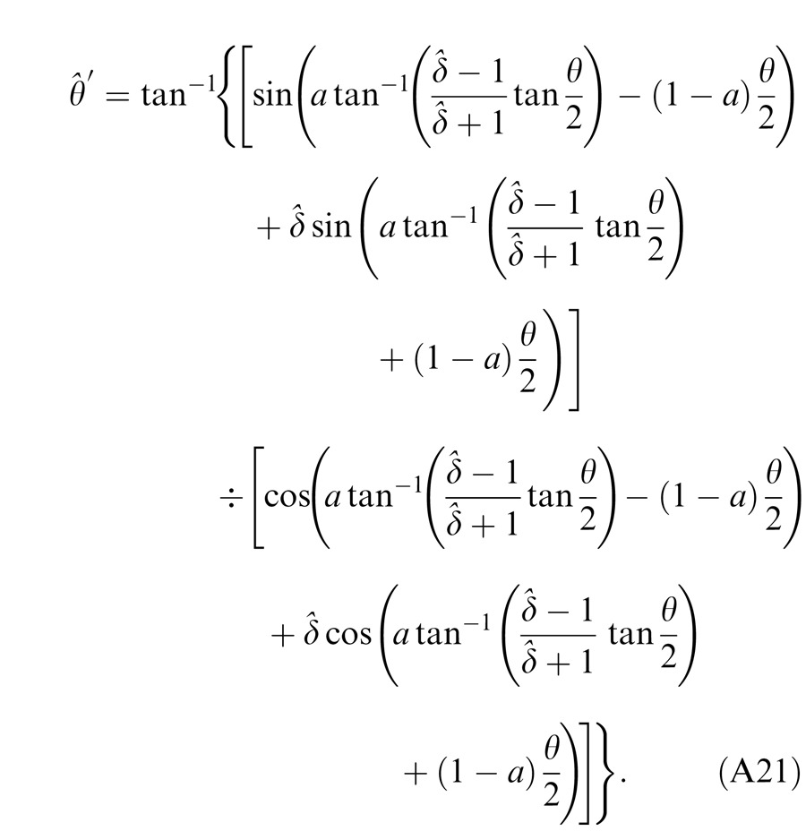Model 2: Ding-Sperling model

Using the same way as in Model 1, from Model 2 (Equations 4 and 6), after interocular interaction, the monocular contrast becomes

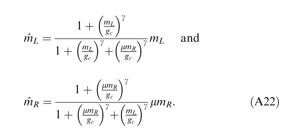Therefore, the apparent interocular contrast ratio is given by

Using Equations A22 and A23, we can calculate the perceived contrast and phase after motor/sensory fusion from Equations A18–A21.

Model 3a: Adding asymmetry between two gain-control layers to the model

From Model 3a (Equations 4 and 7), we can deduce its output monocular contrast to be

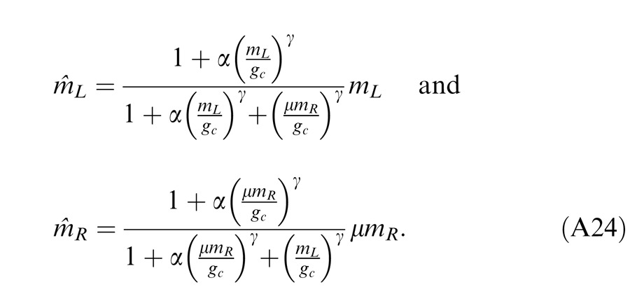Therefore, the apparent interocular contrast ratio is given by

Again, using Equations A24 and A25, the perceived contrast and phase after motor/sensory fusion can be calculated from Equations A18–A21.

Model 3b. Adding interocular gain enhancement to the model

From Model 3b (Equations 4, 8, and 9), we can deduce its output monocular contrast to be

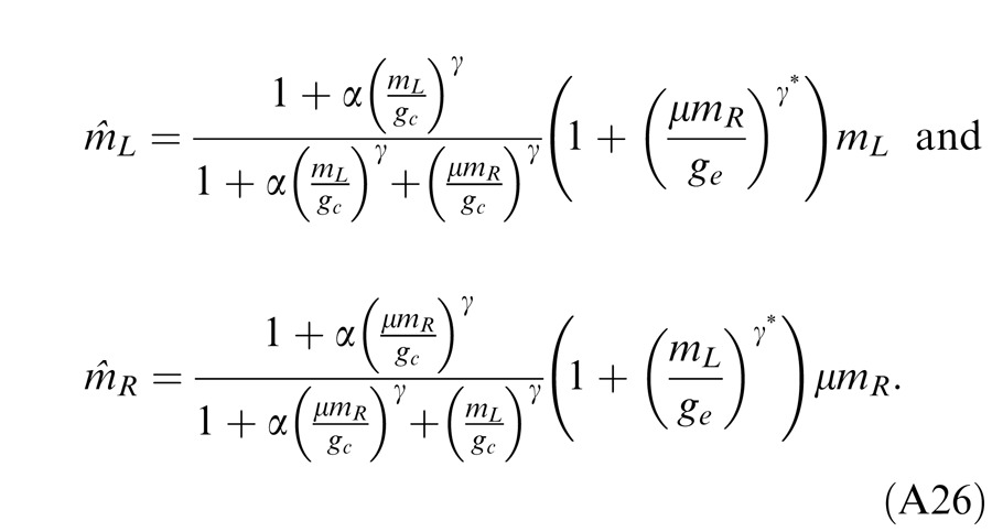Therefore, the apparent interocular contrast ratio is given by

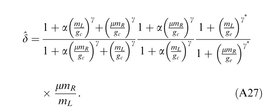Again, using Equations A26 and A27, the perceived contrast and phase can be calculated from Equations A18–A21.

Model 3c: Full model (DSKL model): Adding a mutual inhibition to a gain enhancement

From Model 3c (Equations 4, 9, and 10), we can deduce its output monocular contrast to be

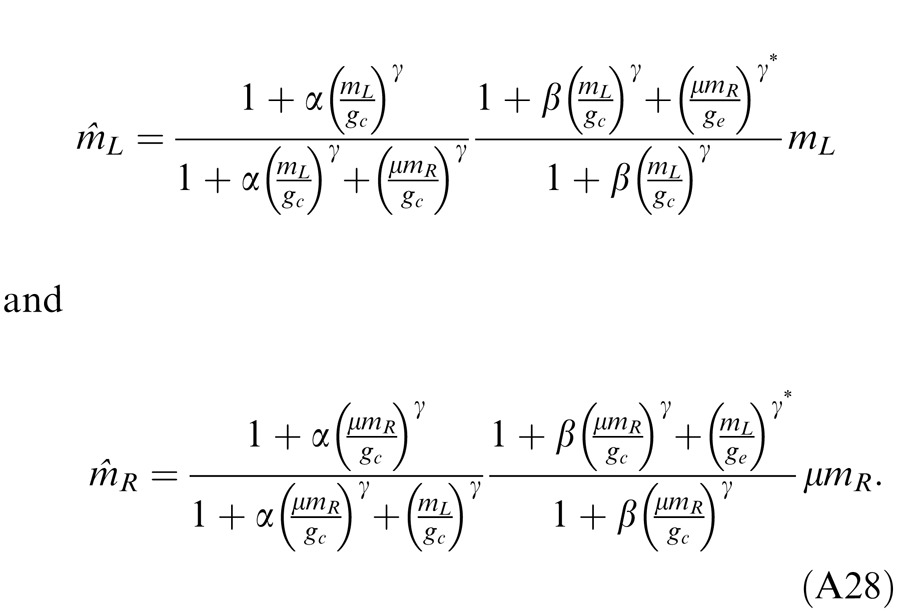Therefore, the apparent interocular contrast ratio is given by

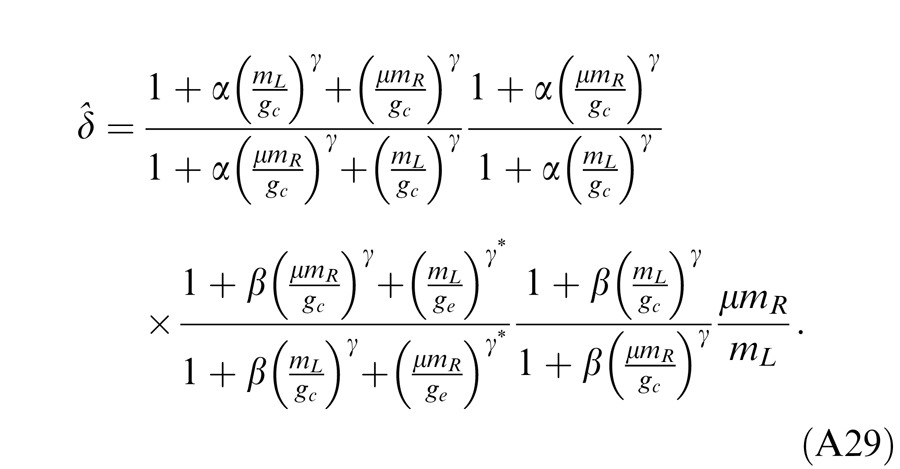Similarly as before, using Equations A28 and A29, the perceived contrast and phase after motor/sensory fusion can be calculated from Equations A18–A21.

Model fitting

We proposed five models in a series with a previous one to be nested within its successor. In Experiment 1, the independent variables are base contrast m = max{m_L, m_R}, interocular contrast ratio δ = m_R/m_L, and two eyes phase difference θ = θ_R – θ_L. At each set of m, δ, θ, we measured the perceived phase ${\mathrm{\theta ˆ}}^{″}$ with standard error of ${{\mathrm{\theta ˆ}}^{″}}_{se}$. On the other side, the perceived phase could be predicted from one of five models, which could be written as a function of m, δ, and θ, i.e.,

In Experiment 2, for each combination of standard contrast m_st, interocular contrast ratio δ = m_R/m_L, and interocular phase difference θ, we measured the base contrast m¯″ = max{m_L, m_R} with standard error of ${{\mathrm{m¯}}^{″}}_{se}$ at a fixed contrast ratio δ when the perceived contrast m¯′ matches the perception ${{\mathrm{mˆ}}^{\prime }}_{st}$ of the standard contrast, i.e., ${{\mathrm{mˆ}}^{\prime }}_{st}$ = ${\mathrm{mˆ}}^{\prime }$. However, all five models in this article have no assumption for monocular contrast perception; they only deal with interocular interactions. When a standard contrast was only presented in the LE, i.e., m_L = m_st and m_R = 0, we have the perception of the standard contrast ${{\mathrm{mˆ}}^{\prime }}_{st}$ = mˆ_st = m_st. On the other side, at a combination of base contrast mˆ, contrast ratio δ, and phase difference θ the perceived contrast mˆ′ could be written as of function of mˆ, δ and θ from a model. When it matches the perception of the standard contrast ${{\mathrm{mˆ}}^{\prime }}_{st}$, we have

From Equation A31, at a fixed contrast ratio δ and a fixed phase difference θ, the base contrast at which the binocular-combined contrast matches monocular standard contrast could be calculated from a model, i.e.,

To minimize the weighted sum of squared errors given by

where θˆ′ and m¯ were predicted from a model given by Equations A30 and A32, respectively, θˆ″ and ${{\mathrm{\theta ˆ}}^{″}}_{se}$ were measured in Experiment 1, and m¯″ and ${{\mathrm{mˆ}}^{″}}_{se}$ were measured in Experiment 2, we could fit the model simultaneously to both phase and contrast data. When spatial frequency varies, the contrast energy might also vary. For each spatial frequency f_s, we have one set of model parameters, g_c and g_e, for computation of contrast energy. For three spatial frequencies, we fit the model to all data for all three spatial frequencies from both experiments by minimizing the weighted sum of squared errors given by

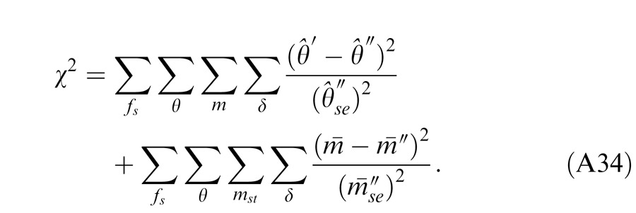Here, we take Model 1 as an example to demonstrate the process of data fitting when the contrast matching experiment was performed only when the two eyes' sine waves were in phase, i.e., mˆ′ = mˆ. Because we always have θˆ′ ≈ θˆ, for simplicity, we only show how to fit Model 1 without considering motor/sensory fusion. From Equations A17 and A18, we have

for prediction of the perceived phase, which is independent of base contrast m in Model 1. For contrast matching experiment, at base contrast m¯, we have m_L = m¯ and m_R = δm¯ when δ ≤ 1, and m_L = m¯/δ and m_R = δ when δ = > 1. From Equations A16 and A20 with θ = 0, the perceived contrast is given by

From Equation A31 and mˆ′ = mˆ_st, the base contrast at which the binocular-combined contrast matches the monocular standard contrast is given by

Applying Equations A35 and A37 in a chi-squared estimator (Equation A33 or A34), we could fit both phase and contrast data into Model 1 without considering motor/sensory fusion. Generally, it would be difficult to write down the explicit formula for Equation A33 or A34, and we had to use Matlab program to find a digital solution of m¯ at a combination of m_st, δ, and θ.

Legge model

For models that were deduced from contrast combination of two in-phase sine waves, we only compared them with our models when the two eyes' sine waves are in phase for binocular contrast combination. Let the two eyes' input sine waves be given by Equations A1 and A2. In the Legge model (Figure 14A), after the calculation of (·)^γ that only operates on contrast and has no effect on phase, the two eye inputs become

Therefore, the apparent interocular contrast ratio is given by

When θ_R – θ_L = θ, from Equations A18 and A39, the perceived phase is given by

The calculation after the binocular combination has no effect on the perceived phase. When the two inputs have identical phase, i.e., θ_L = θ_R, after the combination and the calculation of (·)^1/γ, the perceived contrast is given by

When the standard contrast m_st is only presented in one eye, say, m_L = m_st and m_R = 0, we have its perception mˆ_st = m_st Like the five models in this study, the Legge model doesn't include any monocular mechanism, but unlike these models, it doesn't include any interocular mechanism either. Similarly, as was the case in deducing Equation A37, the base contrast m¯, at which the binocular-combined contrast matches the monocular standard contrast, is given by

Applying Equations A40 and A42 in a chi-squared estimator (Equation A33 with θ = 0 in the second term), we fitted the Legge model to both phase and contrast data at 48% contrast and 0.68 cpd of spatial frequency (blue curve in Figure 15).

Normalization model

The normalization model (Figure 14B) has both signal and control paths in each eye. The signal path is similar to the Legge model except its gain is controlled. In the control path, the contrast is first extracted from each eye's image, pooled together, and then exerts inhibitory gain control to each eye's signal path separately. After these operations, the two eye inputs become

The apparent interocular contrast ratio is still given by Equation A39, and the perceived phase is also given by Equation A40. When θ_L = θ_R, the perceived contrast is given by,

The monocular contrast perception of m_st is given by

Unlike the five models in this article and the Legge model, the normalization model includes monocular contrast gain control. When the perceived contrast at m_L = m¯ and m_R = δm¯ (δ ≤ 1) is matched to mˆ_st, we have

Obviously, we have $m_{st}^{\gamma }$ = (1 + δ^γ)m¯^γ when δ ≤ 1. Similarly, we have $m_{st}^{\gamma }$ = (1 + δ^−γ)m¯^γ when δ > 1. Therefore, we also have Equation A42 in the normalization model to predict the base contrast m¯ when binocularly-combined contrast matches the monocular standard contrast. The model-fitting curve is exactly the same as the one from the Legge model (blue in Figure 15).

Normalization model with asymmetric monocular and interocular gain controls

To include interocular mechanism, monocular and interocular gain controls should have different weights in the normalization model, i.e., after normalization, the apparent monocular contrast is given by

where w is the relative weight for interocular gain control when the weight for monocular gain control is assumed to be one. Therefore, the perceived contrast is given by

And the apparent interocular contrast ratio is given by

Using Equation A49, the perceived phase is given by Equation A18.

References

- Akaike H. (1974). A new look at the statistical model identification. Automatic Control, IEEE Transactions on, 19 (6), 716– 723. [Google Scholar]
- Anderson P. A., Movshon J. A. (1989). Binocular combination of contrast signals. Vision Research , 29 (9), 1115– 1132. [DOI] [PubMed] [Google Scholar]
- Baker D. H., Meese T. S., Georgeson M. A. (2007). Binocular interaction: Contrast matching and contrast discrimination are predicted by the same model. Spatial Vision , 20 (5), 397– 413. [DOI] [PubMed] [Google Scholar]
- Baker D. H., Wallis S. A., Georgeson M. A., Meese T. S. (2012). The effect of interocular phase difference on perceived contrast. PLoS One , 7 (4), e34696. [DOI] [PMC free article] [PubMed] [Google Scholar]
- Banton T., Levi D. M. (1991). Binocular summation in vernier acuity. Journal of the Optical Society of America A , 8 (4), 673– 680. [DOI] [PubMed] [Google Scholar]
- Bearse M. A., Jr., Freeman R. D. (1994). Binocular summation in orientation discrimination depends on stimulus contrast and duration. Vision Research , 34 (1), 19– 29. [DOI] [PubMed] [Google Scholar]
- Blake R., Fox R. (1973). The psychophysical inquiry into binocular summation. Attention, Perception, & Psychophysics, 14 (1), 161– 185. [Google Scholar]
- Blake R., Sloane M., Fox R. (1981). Further developments in binocular summation. Attention, Perception, & Psychophysics, 30 (3), 266– 276. [DOI] [PubMed] [Google Scholar]
- Blake R., Wilson H. (2011). Binocular vision. Vision Research , 51 (7), 754– 770. [DOI] [PMC free article] [PubMed] [Google Scholar]
- Brainard D. H. (1997). The Psychophysics Toolbox. Spatial Vision, 10 (4), 433– 436. [PubMed] [Google Scholar]
- Busettini C., Fitzgibbon E. J., Miles F. A. (2001). Short-latency disparity vergence in humans. Journal of Neurophysiology , 85 (3), 1129– 1152. [DOI] [PubMed] [Google Scholar]
- Campbell F. W., Green D. G. (1965). Monocular versus binocular visual acuity. Nature , 208 (5006), 191– 192. [DOI] [PubMed] [Google Scholar]
- Cannon M. W., Fullenkamp S. C. (1993). Spatial interactions in apparent contrast: Individual differences in enhancement and suppression effects. Vision Research , 33 (12), 1685– 1695. [DOI] [PubMed] [Google Scholar]
- Cogan A. I. (1987). Human binocular interaction: Towards a neural model. Vision Research , 27 (12), 2125– 2139. [DOI] [PubMed] [Google Scholar]
- Cohn T. E., Lasley D. J. (1976). Binocular vision: Two possible central interactions between signals from two eyes. Science , 192 (4239), 561– 563. [DOI] [PubMed] [Google Scholar]
- Ding J., Klein S., Levi D. (2013). Binocular combination in abnormal binocular vision. Journal of Vision , 13 (2): 13: 1– 31, http://www.journalofvision.org/content/13/2/14, doi:10.1167/13.2.14. [DOI] [PMC free article] [PubMed] [Google Scholar]
- Ding J., Klein S., Levi D. (2009). Binocular combination in amblyopic vision. Journal of Vision , 9 (8): 13 http://www.journalofvision.org/content/9/8/274, doi:10.1167/9.8.274 [Abstract] [DOI] [PMC free article] [PubMed] [Google Scholar]
- Ding J., Sperling G. (2006). A gain-control theory of binocular combination. Proceedings of the National Academy of Sciences of the USA , 103 (4), 1141– 1146. [DOI] [PMC free article] [PubMed] [Google Scholar]
- Ding J., Sperling G. (2007). Binocular combination: Measurements and a model. In Harris L., Jenkin M. (Eds.), Computational Vision in Neural and Machine Systems (pp. 257– 305). Cambridge, UK: Cambridge Unversity Press. [Google Scholar]
- Ejima Y., Takahashi S. (1985). Apparent contrast of a sinusoidal grating in the simultaneous presence of peripheral gratings. Vision Research , 25 (9), 1223– 1232. [DOI] [PubMed] [Google Scholar]
- Fogt N., Jones R. (1998a). Comparison of fixation disparities obtained by objective and subjective methods. Vision Research , 38 (3), 411– 421. [DOI] [PubMed] [Google Scholar]
- Fogt N., Jones R. (1998b). The effect of forced vergence on retinal correspondence. Vision Research , 38 (18), 2711– 2719. [DOI] [PubMed] [Google Scholar]
- Fry G. A., Bartley S. H. (1933). The brilliance of an object seen binocularly. American Journal of Ophthalmology , 16, 687– 693. [Google Scholar]
- Huang C. B., Zhou J., Lu Z. L., Feng L., Zhou Y. (2009). Binocular combination in anisometropic amblyopia. Journal of Vision, 9 (3): 13 11– 16, http://www.journalofvision.org/content/9/3/17, doi:10.1167/9.3.17 [PubMed] [Article] [DOI] [PMC free article] [PubMed] [Google Scholar]
- Huang C. B., Zhou J., Lu Z. L., Zhou Y. (2011). Deficient binocular combination reveals mechanisms of anisometropic amblyopia: Signal attenuation and interocular inhibition. Journal of Vision , 11 (6): 13 1– 17, http://www.journalofvision.org/content/11/6/4, doi:10.1167/11.6.4 [PubMed] [Article] [DOI] [PMC free article] [PubMed] [Google Scholar]
- Huang C. B., Zhou J., Zhou Y., Lu Z. L. (2010). Contrast and phase combination in binocular vision. PLoS One, 5 (12), e15075. [DOI] [PMC free article] [PubMed] [Google Scholar]
- Hyson M. T., Julesz B., Fender D. H. (1983). Eye movements and neural remapping during fusion of misaligned random-dot stereograms. Journal of the Optical Society of America , 73 (12), 1665– 1673. [DOI] [PubMed] [Google Scholar]
- Klein S. A. (2001). Measuring, estimating, and understanding the psychometric function: A commentary. Attention, Perception, & Psychophysics, 63 (8), 1421– 1455. [DOI] [PubMed] [Google Scholar]
- Kontsevich L. L., Tyler C. W. (1994). Analysis of stereothresholds for stimuli below 2.5 c/deg. Vision Research , 34 (17), 2317– 2329. [DOI] [PubMed] [Google Scholar]
- Legge G. E. (1981). A power law for contrast discrimination. Vision Research , 21 (4), 457– 467. [DOI] [PubMed] [Google Scholar]
- Legge G. E. (1984a). Binocular contrast summation--I. Detection and discrimination. Vision Research , 24 (4), 373– 383. [DOI] [PubMed] [Google Scholar]
- Legge G. E. (1984b). Binocular contrast summation--II. Quadratic summation. Vision Research , 24 (4), 385– 394. [DOI] [PubMed] [Google Scholar]
- Legge G. E., Rubin G. S. (1981). Binocular interactions in suprathreshold contrast perception. Perception & Psychophysics , 30 (1), 49– 61. [DOI] [PubMed] [Google Scholar]
- Li Z., Atick J. J. (1994). Efficient stereo coding in the multiscale representation*. Network: Computation in Neural Systems , 5 (2), 157– 174. [Google Scholar]
- Mansfield J. S., Legge G. E. (1996). The binocular computation of visual direction. Vision Research , 36 (1), 27– 41. [DOI] [PubMed] [Google Scholar]
- Masson G., Busettini C., Miles F. (1997). Vergence eye movements in response to binocular disparity without depth perception. Nature , 389, 283. [DOI] [PubMed] [Google Scholar]
- Meese T. S., Georgeson M. A., Baker D. H. (2006). Binocular contrast vision at and above threshold. Journal of Vision, 6 (11): 13 1224– 1243, http://www.journalofvision.org/content/6/11/7, doi:10.1167/6.11.7 [PubMed] [Article] [DOI] [PubMed] [Google Scholar]
- Meese T. S., Hess R. F. (2004). Low spatial frequencies are suppressively masked across spatial scale, orientation, field position, and eye of origin. Journal of Vision, 4 (10): 13 843– 859, http://www.journalofvision.org/content/4/10/2, doi:10.1167/4.10.2 [PubMed] [Article] [DOI] [PubMed] [Google Scholar]
- Moradi F., Heeger D. J. (2009). Inter-ocular contrast normalization in human visual cortex. Journal of Vision , 9 (3): 13 1– 22, http://www.journalofvision.org/content/9/3/13, doi:10.1167/9.3.13 [PubMed] [Article] [DOI] [PMC free article] [PubMed] [Google Scholar]
- Nachmias J. (2006). The role of virtual standards in visual discrimination. Vision Research , 46 (15), 2456– 2464. [DOI] [PubMed] [Google Scholar]
- Panum P. L. (1858). Physiologische Untersuchungen über das Sehen mit zwei Augen (Physiological Investigations Concerning Vision with Two Eyes). Kiel, Germany: Schwerssche Buchandlung. [Google Scholar]
- Pelli D. G. (1997). The Video Toolbox software for visual psychophysics: Transforming numbers into movies. Spatial Vision, 10 (4), 437– 442. [PubMed] [Google Scholar]
- Pelli D. G., Zhang L. (1991). Accurate control of contrast on microcomputer displays. Vision Research , 31 (7), 1337– 1350. [DOI] [PubMed] [Google Scholar]
- Richards W. (1968). Spatial remapping in the primate visual system. Biological Cybernetics, 4 (4), 146– 156. [DOI] [PubMed] [Google Scholar]
- Schor C., Wood I., Ogawa J. (1984). Binocular sensory fusion is limited by spatial resolution. Vision Research , 24 (7), 661– 665. [DOI] [PubMed] [Google Scholar]
- Sheliga B. M., Chen K. J., Fitzgibbon E. J., Miles F. A. (2005). Short-latency disparity vergence in humans: Evidence for early spatial filtering. Annals of the New York Academy of Sciences , 1039 (1), 252– 259. [DOI] [PMC free article] [PubMed] [Google Scholar]
- Sheliga B. M., Fitzgibbon E. J., Miles F. A. (2006). Short-latency disparity vergence eye movements: A response to disparity energy. Vision Research, 46 (21), 3723– 3740. [DOI] [PMC free article] [PubMed] [Google Scholar]
- Sheliga B. M., Fitzgibbon E. J., Miles F. A. (2007). Human vergence eye movements initiated by competing disparities: Evidence for a winner-take-all mechanism. Vision Research , 47 (4), 479– 500. [DOI] [PMC free article] [PubMed] [Google Scholar]
- Ukwade M. T. (2000). Effects of nonius line and fusion lock parameters on fixation disparity. Optometry & Vision Science , 77 (6), 309– 320. [DOI] [PubMed] [Google Scholar]
- Wilson H. R. (2003). Computational evidence for a rivalry hierarchy in vision. Proceedings of the National Academy of Sciences of the USA , 100 (24), 14499– 14503. [DOI] [PMC free article] [PubMed] [Google Scholar]
- Xing J., Heeger D. J. (2001). Measurement and modeling of center-surround suppression and enhancement. Vision Research , 41, 571– 583. [DOI] [PubMed] [Google Scholar]
- Yeshurun Y., Carrasco M., Maloney L. T. (2008). Bias and sensitivity in two-interval forced choice procedures: Tests of the difference model. Vision Research , 48 (17), 1837– 1851. [DOI] [PMC free article] [PubMed] [Google Scholar]