Binocular combination in abnormal binocular vision

Abstract

We investigated suprathreshold binocular combination in humans with abnormal binocular visual experience early in life. In the first experiment we presented the two eyes with equal but opposite phase shifted sine waves and measured the perceived phase of the cyclopean sine wave. Normal observers have balanced vision between the two eyes when the two eyes' images have equal contrast (i.e., both eyes contribute equally to the perceived image and perceived phase = 0°). However, in observers with strabismus and/or amblyopia, balanced vision requires a higher contrast image in the nondominant eye (NDE) than the dominant eye (DE). This asymmetry between the two eyes is larger than predicted from the contrast sensitivities or monocular perceived contrast of the two eyes and is dependent on contrast and spatial frequency: more asymmetric with higher contrast and/or spatial frequency. Our results also revealed a surprising NDE-to-DE enhancement in some of our abnormal observers. This enhancement is not evident in normal vision because it is normally masked by interocular suppression. However, in these abnormal observers the NDE-to-DE suppression was weak or absent. In the second experiment, we used the identical stimuli to measure the perceived contrast of a cyclopean grating by matching the binocular combined contrast to a standard contrast presented to the DE. These measures provide strong constraints for model fitting. We found asymmetric interocular interactions in binocular contrast perception, which was dependent on both contrast and spatial frequency in the same way as in phase perception. By introducing asymmetric parameters to the modified Ding-Sperling model including interocular contrast gain enhancement, we succeeded in accounting for both binocular combined phase and contrast simultaneously. Adding binocular contrast gain control to the modified Ding-Sperling model enabled us to predict the results of dichoptic and binocular contrast discrimination experiments and provides new insights into the mechanisms of abnormal binocular vision.

Introduction

As many as 1 in 20 people have defective stereovision (Stelmach & Tam, 1996), often as a consequence of compromised binocular visual experience early in life. For example, roughly 3% of the population has amblyopia, with reduced visual acuity, contrast sensitivity, and positional acuity in their nondominant eye (NDE) and abnormal binocular vision (McKee, Levi, & Movshon, 2003). There are also stereoblind individuals who have normal monocular visual functions but have abnormal binocular vision (Lema & Blake, 1977).

For persons with amblyopia, under normal viewing conditions the NDE is suppressed (Li et al., 2011) and fusion and stereopsis are compromised (Lema & Blake, 1977; Levi, Harwerth, & Manny, 1979; Levi, Harwerth, & Smith, 1980; McKee et al., 2003). Binocular vision in amblyopia is not only affected by abnormal monocular inputs from the NDE (Harrad & Hess, 1992), but the development of the binocular system itself may also be compromised. According to physiological studies, most neurons in normal primary visual cortex receive their inputs from both eyes. Although these binocular connections are functionally present at or shortly after birth, their maintenance and refinement are highly dependent on normal binocular experience (Chino, Smith, Hatta, & Cheng, 1997; Freeman & Ohzawa, 1992; Horton & Hocking, 1996). In animals deprived of normal binocular vision (lens- or prism-reared) during a sensitive period, fewer neurons have balanced ocular dominance and a larger proportion of neurons are excited by only one eye (Smith et al., 1997).

While amblyopia results in reduced acuity and contrast sensitivity in the NDE, some amblyopic individuals lack binocular motion integration and stereovision even after compensating for the reduced contrast sensitivity (McKee et al., 2003). However, Baker, Meese, Mansouri, and Hess (2007) reported that some individuals with strabismic amblyopia demonstrate summation of the two eyes' inputs beyond probability summation after normalizing monocular contrast sensitivities. Goodman, Black, Phillips, Hess, and Thompson (2011) demonstrated two cases of excitatory binocular interactions in individuals with alternating fixation when balanced vision was achieved by decreasing the DE's contrast.

Although many V1 neurons appeared to be monocular in amblyopic vision, they exhibit clear interocular interactions—primarily suppression—during dichoptic stimulation (Smith et al., 1997). Indeed, neurons in areas V1 and V2 of monkeys with strabismic amblyopia show substantially increased binocular suppression (Bi et al., 2011).

Psychophysical studies also showed evidence of interocular interactions in amblyopic vision, including transfer of visual aftereffects (Harwerth & Levi, 1983; McKee et al., 2003) and dichoptic masking (Harrad & Hess, 1992; Harwerth & Levi, 1983; Holopigian, Blake, & Greenwald, 1988). These interactions may be asymmetric across the two eyes. For example, dichoptic contrast masking studies revealed stronger suppression from the DE to the NDE than vice versa (Harrad & Hess, 1992; Harwerth & Levi, 1983; Holopigian et al., 1988). However, Baker, Meese, and Hess (2008) gave an alternative interpretation of their dichoptic contrast masking data. Their two-stage model (Meese, Georgeson, & Baker, 2006) predicts that the magnitude of masking remains similar across the two eyes even when the weights of interocular gain control differ by a factor of 10 and thus failed to account for asymmetric dichoptic masking in amblyopic vision. In order to successfully model their data, they included attenuation of the signal and an increase in noise in the NDE in their two-stage model, with interocular suppression intact. Based on their modeling, they concluded that there is attenuation of the signal and an increase in noise in the amblyopic eye, with intact stages of interocular suppression and binocular summation.

A different approach to studying suprathreshold binocular interactions involves measuring the perceived phase of a cyclopean sine wave. This paradigm, introduced by Ding and Sperling (2006, and see the preceding article), has recently been used in studying suprathreshold binocular combination in amblyopic vision (Ding, Klein, & Levi, 2009; Huang, Zhou, Lu, Feng, & Zhou, 2009; Huang, Zhou, Lu, & Zhou, 2011). In this paradigm, horizontal suprathreshold sinusoids are presented separately to the two eyes, one with phase set to 45° and the other to −45°, and the observer is required to judge the perceived phase of the cyclopean grating. Normal observers judge the perceived phase of the cyclopean grating to be zero when the two eyes are presented with gratings of identical contrast—i.e., they have balanced vision when identical contrast is presented to the two eyes. However, for amblyopic observers to attain balanced vision between two eyes, the NDE needs to be presented with a higher contrast image (Ding et al., 2009; Huang et al., 2009). Indeed, the NDE requires higher contrast than one would predict from either the difference in monocular perceived contrast or contrast sensitivities of the two eyes—presumably because the DE exerts stronger suppression to the NDE than vice versa. Ding et al. (2009) also found that this asymmetric interocular suppression was dependent on the base contrast (the higher of the two eyes' contrasts) of the sine wave. At a constant interocular contrast ratio, when the base contrast increased, the DE-to-NDE suppression increased more than the NDE-to-DE suppression, shifting the perceived phase more toward the DE at higher base contrast than at lower base contrast. This observation was later confirmed by Huang et al. (2011). The Ding-Sperling model with asymmetric model parameters was used to account for binocular combination in amblyopic vision (Ding et al., 2009; Huang et al., 2011). Although the model can account for many features of both normal and anisometropic amblyopic binocular combination data, it failed to pick up a feature found in data for some of the abnormal observers of Ding et al. (2009). Specifically, when the DE's contrast was held constant while the NDE's contrast increased, the perceived phase shifted to the DE, an apparent contrast enhancement from the NDE to DE. In order to account for this interocular contrast enhancement, we proposed a gain-control and gain-enhancement model, the DSKL model in the preceding article (Ding, Klein, & Levi, 2013) by explicitly including interocular enhancement—multiplying the other eye's contrast in one eye's gain operator.

In the present study, we measured both binocular phase and contrast combination data in separate experiments in observers with abnormal binocular visual experience early in life. Similar experiments were reported by Huang et al. (2011) in four observers with anisometropic amblyopia. We compare five models proposed in the preceding article to simultaneously fit both the phase and contrast combination data of our observers with abnormal binocular vision. Additionally, we compare our models with other extant models for binocular combination. We find that the DSKL model provides the best fit to both the phase and contrast data. By adding a binocular gain control to the DSKL model we are also able to predict the results of monocular, dichoptic, and binocular contrast discrimination experiments (Baker et al., 2008; Meese et al., 2006).

Most of phase data in this study were presented as a poster at Vision Sciences Society in 2009 (Ding et al., 2009). All the contrast data and many aspects of the modeling are new.

Methods

Stimuli and procedures are identical to those described in the preceding article (Ding, Klein, & Levi, 2013) except that, in order to assist an amblyopic observer to align and fuse the two eyes' images, the contrast of the binocular fusion-assisting frame in the DE was reduced until both eyes were able to see and fuse the frames (Ding & Levi, 2011). For some of the abnormal observers, binocular alignment and fusion training was necessary before starting the experiment. Only after observers could report a steady dichoptic cross were the data used for further analysis. Four observers who failed to obtain binocular alignment and fusion after training were excluded from the study.

Experimental conditions

In Experiment 1, we measured the perceived phase of the binocularly-combined cyclopean sine wave when the base contrast, m = max{m_d, m_n}, varied from 6% to 96%, interocular contrast ratio of NDE to DE, δ = m_n/m_d, varied from ¼ to 32, the spatial frequencies were 0.68, 1.36, or 2.72 cpd (obtained by varying the viewing distance), and the phase difference, θ = |θ_n – θ_d|, was fixed at 90° in most cases but was varied (45°, 90°, and 135°) for one abnormal observer at spatial frequency of 1.36 cpd.

Figure 1A shows the test points of NDE versus DE contrast, at which the perceived phase was measured. Points along one solid curve have the same base contrasts m and points along a dashed line have the same interocular contrast ratio δ that is labeled near the line.

Figure 1.

Experimental points in the NDE versus DE contrast plane. (A) Solid lines connect points of the same base contrast (0.06, 0.12, 0.24, 0.48, and 0.96), higher contrast in the two eyes, and dashed lines connect points of the same interocular contrast ratio, NDE/DE (labeled near the line) in the range from ¼ to 32. (B) Regrouping measuring points in the NDE versus DE contrast plane into two conditions: (1) DE (LE) contrast remains constant (vertical red line) and (2) NDE (RE) contrast remains constant, when interocular contrast ratio NDE/DE (RE/LE) varies in the range from ¼ to 16.

In Experiment 2, we measured the perceived contrast of a binocularly-combined cyclopean sine wave. On each trial, the standard sine wave was presented to the DE in either the first or second interval, and the test contrast was presented to both eyes with the interocular contrast ratio varying from trial to trial. The observer's task was to judge which interval had the sine wave with higher contrast. We tested 11 interocular contrast ratios at each standard contrast (48%, 24%, or 12%).

Staircases

Each staircase was run for 50 trials. For one run, the spatial frequency, phase difference, and the base contrast were fixed, but the interocular contrast ratio varied, i.e., the points along one solid line in Figure 1A were tested randomly. In Experiment 1, for each interocular contrast ratio, there were two displays, one with the NDE's sine wave shifted up (45 phase degree) and one with the NDE's sine wave shifted down (−45 phase degree) (see preceding article). Two staircases were interleaved to measure the perceived phase of the two displays, and the average perceived phase, θˆ = (θˆ₁ − θˆ₂)/2, was calculated as the dependent variable of the experiment. Typically, for each run, there were 28 concurrent staircases interleaved to measure the perceived phase for 14 interocular contrast ratios. A total of 3 (Spatial Frequency) × 6 (Base Contrast) × 14 (Contrast Ratio) × 2 (Displays) × 50 (Repeats) = 25,200 trials were run for an observer tested on three spatial frequencies, and the total of 1 × 6 × 14 × 2 × 50 = 8,400 trials were run for an observer tested on one spatial frequency.

In Experiment 2, for one run, the spatial frequency and the standard contrast were fixed, but interocular contrast ratios were randomly interleaved. For each contrast ratio, two staircases were interleaved for the contrast matching task, one for the standard contrast being in the first interval and one for the standard contrast being in the second interval. The dependent variable was the average of contrast measured in the two staircases. There were 22 concurrent staircases interleaved for each run. The total of 3 (Spatial Frequency) × 2–4 (Standard Contrast) × 1–4 (Phase) × 11 (Contrast Ratio) × 2 (One Staircase for Each Temporal Position of the Standard) × 50 (Repeats) = 6,600 or 30,800 trials were run for observer GJ or GD, 1 × 1 × 11 × 2 × 50 = 1,100 trials were run for observer AB, BK, PB, or MY.

Observers

The abnormal observers in this study are the same as those presented in Ding et al. (2009). Six observers signed the written consent and participated in the experiment. Clinical details are provided in Table 1. Before the experiment, one training session, with the sine-wave grating only presented to one eye (control conditions), was run to test whether an observer could perform the task. Two observers who failed the control condition test (failed to see the NDE image while the DE was open) were excluded from further experiments. Observers who had difficulties in binocular alignment and fusion at higher spatial frequencies only performed the task at 0.68 cpd.

Table 1.

Clinical data for strabismic/amblyopic observers. Notes: Aniso, anisometropia; Strab, Strabismus; ET, esotropia; XT, exotropia; HyperT, hypertropia; Δ, prism dioptres; A, alternating; DE, dominant eye; NDE, nondominant eye.

	Age	Gender	Type	Strabismus	Stereo	Eye	Refractive error	Letter acuity (Snellen)
GJ	25	M	Strab & aniso	R ET 4 Δ		R(NDE) L(DE)	+3.00/−0.50 × 90 plano/−0.25 × 90	20/40−2 20/16
GD	46	F	Aniso	None	70 arcsec	R(DE) L(NDE)	+0.25/−0.50 × 90 +3.75/−1.00 × 30	20/12.5−2 20/50+2
AB	24	F	Strab & aniso	A ET 9 Δ R HyperT 8 Δ		R(NDE) L(DE)	−3.75 −6.25	20/20 20/20
BK	62	M	Strab & aniso	A XT 8 Δ L HyperT 7 Δ		R(DE) L(NDE)	−1.50/−2.50 × 105 −3.00/−0.25 × 135	20/12.5−1 20/25+1
MY	34	F	Strab & aniso	A XT 7 Δ R HyperT 7 Δ		R(DE) L(NDE)	−2.50/−0.25 × 90 −0.75	20/16 20/16
PB	26	F	Strab	A ET > 15 Δ		R(DE) L(NDE)	+0.50/−1.25 × 105 +0.50/−1.25 × 70	20/16+2 20/25+2

Results

Experiment 1: Perceived phase of binocularly-combined cyclopean sine waves

Figure 2 shows the perceived phase of binocularly-combined cyclopean sine waves as a function of the NDE/DE contrast ratio, δ, for two observers who were able to perform the binocular combination tasks at all three spatial frequencies (0.68, 1.36, and 2.72 cpd—Figure 2A), and for four observers who could only perform the task at the low spatial frequency (0.68 cpd—Figure 2B). The phase difference between the sine waves presented to the two eyes was fixed at 90°; the DE's phase was −45° indicated by arrows on the left side of Figure 2, and the NDE's was 45° indicated by arrows on the right side. The solid curves are the best fits from the DSKL model (Model 3c—see preceding article). The black dashed curve is the prediction from algebraic (linear) summation of two eyes' sine waves with attenuation in the NDE for ocular imbalanced contrast perception, which is the asymptote of Models 2 and 3a–c at zero contrast energy.

Figure 2.

Results of Experiment 1. Perceived phase θˆ of binocularly-combined cyclopean sine waves as a function of the NDE/DE contrast ratio (δ), when the base contrast m is 96% (*), 48% (x), 24% (○), 12% (▿), or 6% (□). (A) Data collected from two observers at three spatial frequencies. The black vertical bars indicate contrast threshold ratios. (B) Data collected from four observers at only one spatial frequency. The phase difference of the two eyes' sine-wave gratings was fixed at 90°; DE's phase was −45° indicated by arrows on the left side and NDE's phase was 45° indicated by arrows on the right side. When δ ≤ 1 the DE's grating contrast was fixed at base contrast m and δ was increased by increasing the NDE's contrast (δ m). When δ ≥ 1 the NDE's contrast remained constant at the base contrast m, and δ was increased by decreasing the DE's contrast (m/ δ). The solid curves are the best fits from the DSKL model. The black dashed curve is the prediction of linear summation with attenuation in the NDE for ocular imbalanced contrast perception, the asymptote of Models 2 and 3a–c at zero contrast energy. The red arrow in the bottom-left plot (PB) indicates two data points at which the DE's contrast was identical at 6%, but the NDE's contrast increased from 24% to 48%. The red arrow in the bottom-right plot (MY) indicates two data points at which the DE's contrast was identical at 12%, but the NDE's contrast increased from 48% to 96%.

When the NDE/DE contrast ratio δ increased, the perceived phase shifted from the DE's to the NDE's. However, unlike normal observers (see figure 6 in the preceding article), abnormal observers had strong eye biases; almost all the data points fall below the linear summation lines (black dashed lines), indicating a strong bias toward the DE in suprathreshold binocular phase combination. This DE bias is dependent on both the base contrast and spatial frequency: more biased to the DE at higher base contrasts and at higher spatial frequencies. When the base contrast increased from 6% to 96%, the size of the DE-bias consistently increased. At 96% (red symbols), the NDE made almost no contribution to the perceived phase when the two eyes were presented with identical contrast (δ = 1, vertical dashed line in Figure 2)—it was almost completely suppressed by the DE. In order for the NDE's image to contribute to the cyclopean percept, the DE's contrast has to be reduced (NDE/DE ratio increased) and the perceived phase then shifted from DE-biased (θˆ < 0) to NDE-biased (θˆ > 0).

Normal observers have balanced vision between the two eyes when the two eyes' sine waves have equal contrast (contrast ratio = one), i.e., both eyes contribute equally to the perceived cyclopean sine wave and the perceived phase θˆ = 0) when the two eyes' sine waves have equal but opposite phase shifts (see preceding article). For abnormal observers, the apparent balance point (θˆ = 0) reflects the NDE/DE contrast ratio at which both eyes contribute equally to the binocular combination (the intercept of a fitting curve with the horizontal dashed line θˆ = 0). We define the NDE/DE contrast ratio at the balance point as the balanced-NDE/DE-ratio (δ_B). When the base contrast increased from 6% to 96%, the data shifted from left to right, i.e., the balanced-NDE/DE-ratio δ_B increased. In other words, the higher the base contrast, the more the DE's contrast needs to be reduced in order to achieve balanced vision. When spatial frequency increased from 0.68 to 2.72 cpd (Figure 2A), the data consistently shifted to the right; in order to achieve balanced vision, the DE contrast must be reduced more at higher spatial frequencies, i.e., higher spatial frequencies have higher balanced-NDE/DE-ratio. At 2.72 cpd (bottom of Figure 2A), when the two eyes were presented with identical contrast (δ = 1, vertical dashed line), the NDE was completely suppressed by the DE at all base contrasts.

The variation in the balanced NDE/DE-ratio (δ_B) can be more easily seen in Figure 3, which plots δ_B at the balance point against NDE contrast. This figure shows clearly that in normal observers (black symbols) δ_B is ≈1 independent of NDE contrast and spatial frequency, whereas in the abnormal observers it is greater than one and increases systematically with both NDE contrast and spatial frequency. For several abnormal observers balanced vision requires an NDE/DE-ratio greater than 10! This strong imbalance is not simply a consequence of reduced contrast perception or elevated contrast thresholds in the NDE. Suprathreshold contrast perception is normal or nearly so in amblyopic eyes (Hess & Bradley, 1980; Loshin & Levi, 1983), and the black bars in Figure 2A show the contrast detection threshold ratios for observers GD and GJ. Their threshold ratios at all three spatial frequencies are close to one (actually less than one at the two lower frequencies), in contrast to the balance ratios of eight (GD) and almost 40 (GJ) at the highest spatial frequency and contrast.

Figure 3.

NDE/DE contrast ratio at balance vision as function of NDE contrast. Black marks demonstrate the RE/LE contrast ratio at balance vision for normal observers (JP and MD) from our preceding article.

The effect of phase

In the experiments thus far, the input phase in the two eyes differed by 90°. In order to examine the effect of input phase on binocular combination, we measured the perceived phase when the two eyes' input phases varied. Figure 4 shows the perceived phase as a function of NDE/DE contrast ratio when the phase difference θ of the two eyes' sine-wave gratings was 45° (top), 90° (middle), or 135° (bottom) for amblyopic observer GD for spatial frequency 1.36 cpd. The data for 90° phase difference are from Figure 2, but replotted on a different scale. Similar to Figure 2, when the NDE/DE ratio increased, the perceived phase shifted from the DE to NDE, i.e., from −22.5° to 22.5° when θ = 45° (top), from −45° to 45° when θ = 90° (middle), or from −67.5° to 67.5° when θ = 135° (bottom). When the base contrast increased from 6% to 96%, the data shifted from left to right consistently at all three input phase differences. The solid curves are the best fits from the DSKL model (see preceding article) with same model parameters for three input phase differences; no extra model parameter is needed for model fitting when the input phase varies.

Figure 4.

The perceived phase as a function of NDE/DE contrast ratio when the phase difference of the two eyes' sine-wave gratings was 45° (top), 90° (middle), and 135° (bottom) for one observer at 1.36 cpd of spatial frequency. The data for 90° phase difference are the same as in Figure 2 but are replotted on a different scale in order to compare with data for 135°.

Interocular enhancement

There are two methods for varying the NDE/DE contrast ratio: (a) varying the NDE's contrast while holding the DE's contrast constant (constant-DE-contrast condition), illustrated by the vertical red line in Figure 1B; (b) varying the DE's contrast while holding the NDE's contrast constant (constant-NDE-contrast condition), shown by the horizontal blue line in Figure 1B. When the DE's contrast remains constant while the NDE's varies, the interaction from DE to NDE should also remain constant and the perceived phase should reflect the interaction from NDE to DE. On the other hand, the perceived phase in the constant-NDE-contrast condition reflects the interaction from DE to NDE. Therefore we can compare interocular interactions by comparing the perceived phase under these two conditions.

By regrouping the measuring points as shown in Figure 1B, we replotted the results for normal (data from the preceding article) and abnormal observers in Figure 5 when DE (LE) contrast remains constant at 6% (red stars) or when NDE (RE) contrast remain constant at 6% (blue squares). For normal observers (Figure 5A), there was almost no difference whether the LE or RE had constant contrast while the other eye's contrast varied; the perceived phase was only dependent on the interocular ratio. This is not surprising because normal observers have symmetric interocular interactions and the data for all base contrasts were almost overlaid (see figure 6 in the preceding article). However, for observers with anomalous binocular vision (Figure 5B), the perceived phase behaved quite differently in the two conditions. For observer GD, under constant-DE-contrast conditions (red), when the NDE's contrast increased the perceived phase was more biased to the NDE than predicted by linear summation (dashed curve), reflecting the effect of suppression from the NDE to DE. However, it was less biased to the NDE than under the constant-NDE-contrast condition (blue), reflecting a smaller effect of suppression from NDE to DE than from DE to NDE. For observer GJ, at 0.68 cpd of spatial frequency, under constant-DE-contrast conditions (red), when the NDE's contrast increased the perceived phase became biased toward the NDE but never beyond the prediction from linear summation (dashed curve), demonstrating that the NDE had no apparent suppressive effect on the DE. Interestingly, for this observer, at 1.36 cpd, when the DE's contrast remained constant and the NDE's contrast increased (red), the perceived phase became more biased toward the DE at high NDE/DE contrast ratios (indicated by red arrows), demonstrating an apparent enhancement effect from the NDE to the DE. Similar NDE-to-DE enhancement could also be observed in the data of two other abnormal observers (see red arrows in the bottom panels of Figure 2B).

Figure 5.

Redrawing the results of Experiment 1 for amblyopes and normal observers when the DE's (LE's) contrast remained constant at 6% (red stars) (constant-DE-contrast condition) or when the NDE's (RE's) contrast remained constant at 6% (blue squares) (constant-NDE-contrast condition). The solid colored curves are the best fit from the DSKL model and the black dashed curve is the prediction of linear summation. Red arrows indicate data points where the perceived phase shifted to the DE when the NDE's contrast increased.

Apparent DE-to-NDE enhancement can be observed directly in Figure 2, when the contrast ratio NDE/DE (δ) ≥ 1 where the data were collected in the constant-NDE-contrast condition. For strabismic observer BK (top-right panel in Figure 2B), when the DE's contrast increased from 0 to 96% and the NDE's contrast remained constant at 96% (red stars from right to left when δ decreased), the perceived phase was first shifted to the DE more rapidly than linear summation predicted, reflecting apparent DE-to-NDE inhibition and then shifted back to the NDE, reflecting apparent DE-to-NDE enhancement. This apparent DE-to-NDE enhancement could also be observed in other strabismic observers' data, although not obviously, but could not be observed in anisometropic observer GD's data (left column in Figure 2A).

Experiment 2: Perceived contrast of binocularly-combined cyclopean sine waves

Figure 6 shows the binocularly equal perceived contrast contours measured when the standard contrast in the DE was 6% (first column), 12% (second column), 24% (third column), or 48% (fourth column), and the spatial frequency was 0.68 (top), 1.36 (middle), or 2.72 cpd (bottom). The two eyes' sine waves were in phase (blue circle), tested for all conditions, 90° (red star) and 135° (black square) out-of-phase, tested for 0.68 and 1.36 cpd, or 45° (green triangle) out-of-phase, tested only at 1.36 cpd and 48% contrast.

Figure 6.

Results of Experiment 2 for observer GD. Binocularly equal-contrast contours obtained by comparing the contrast of a binocularly-combined sine-wave grating with the standard contrast that was always presented in the DE when the NDE/DE contrast ratio was 0, 0.125, 0.25, 0.5, 0.71, 1, 1.4, 2, 4, 8, or ∞. The contrast of a standard grating was 6% (first column), 12% (second column), 24% (third column), or 48% (the fourth column), its spatial frequency was 0.68 (top), 1.36 (middle), or 2.72 cpd (bottom), and interocular phase difference was 0° (blue circle), 45° (green triangle), 90° (red star), or 135° (black square). The solid curve is the best fit from the DSKL model using the same model parameters for fitting data from Experiment 1.

Figure 7 shows results of observer GJ who was tested at all three spatial frequencies with gratings that were in phase and also at 0.68 cpd with 90° out of phase of sine waves at 48% contrast. Figure 8 shows the results of other four strabismic observers who were only tested under very limited conditions, with the two eyes' sine waves always in phase, their spatial frequency fixed at 0.68 cpd, and a standard contrast of 48%.

Figure 7.

Results of Experiment 2 for observer GJ. Binocularly equal-contrast contours obtained by comparing the contrast of a binocularly-combined sine-wave grating with the standard contrast that was always presented in the DE when the NDE/DE contrast ratio was 0, 0.125, 0.25, 0.5, 0.71, 1, 1.4, 2, 4, 8, or ∞. The contrast of a standard grating was 24% (first column) or 48% (second column), and its spatial frequency was 0.68 (top), 1.36 (middle), or 2.72 cpd (bottom). Two eyes' sine waves were in phase (blue circle) tested for all conditions or 90° out of phase (red star) tested only for 0.68 cpd and 48% contrast. The solid curve was the best fit from the DSKL model using the same model parameters for fitting data from Experiment 1.

Figure 8.

Results of Experiment 2 for other four strabismic observers who tested only limited conditions. The contrast of a standard grating was 48%, and its spatial frequency was 0.68 cpd. Two eyes' sine waves were always in phase (blue circle). The solid curve was the best fit from the DSKL model using the same model parameters for fitting data from Experiment 1.

Unlike the results of normal observers in the preceding article, the binocularly equal-contrast contours for abnormal observers are asymmetric; the DE exerted stronger suppression on the NDE than vice versa. When the DE's contrast increased from zero to a small value, in order to have the same perceived binocular contrast, the NDE needed higher contrast than in monocular viewing (this is an example of Fechner's paradox) because of strong DE-to-NDE suppression. However, Fechner's paradox could not be observed when the NDE's contrast increased from zero to a small value; NDE-to-DE suppression was either absent or too weak to be observed. In agreement with the results of Experiment 1, the DE-to-NDE suppression was dependent on base contrast and spatial frequency, stronger at higher base contrasts and also stronger at higher spatial frequencies. Unlike normal observers who demonstrated phase independence in binocular contrast combination at high base contrast (see preceding article and also Huang, Zhou, Zhou, & Lu, 2010), abnormal observers GD and GJ show phase dependence in contrast summation even at high contrast, reflecting their abnormal motor/sensory fusion. The solid curves are the best fit from the DSKL model using the same model parameters as in Experiment 1. The horizontal and vertical dashed lines are predictions from the winner-take-all model; unlike in normal observers, this model fails to predict the contour data for abnormal observers.

Modeling

In the preceding article, we proposed and compared five models with symmetric model parameters in the two eyes to account for normal binocular combination. To account for binocular combination in abnormal binocular vision and amblyopia, we modified these models to allow asymmetric parameters between the two eyes. Below we briefly describe these asymmetric models and discuss how they perform. The Appendix provides the specific details for each of the five asymmetric models. Because all models share the same motor/sensory fusion mechanism that was described in the preceding article (Ding, Klein, & Levi, 2013), here we only compare the interocular interactions of the models. In addition, below, we compare our models with extant models for abnormal binocular vision.

Model 1: Contrast weighted summation model, including asymmetric contrast sensitivity

Is asymmetric contrast sensitivity sufficient to account for the asymmetric interocular interaction in abnormal vision? To answer this question, we only incorporate asymmetric contrast sensitivities in the two eyes in the Ding-Sperling model and assume that the interocular gain controls are symmetric.

Although Huang et al. (2009) used this contrast-weighted summation model to account for binocular phase combination in anisometropic amblyopic vision, we found that this model could be rejected (Ding et al., 2009) for binocular combination in abnormal binocular vision because it failed to account for the increase in DE-to-NDE suppression when the base contrast increased (data were shifted to right in Figure 2); i.e., the balanced-NDE/DE-ratio increased at higher base contrasts. Figure 9A shows the fit of Model 1 to one observer's data. The predicted phase shifts are independent of base contrast and are overlapped with each other, while the actual data shift consistently to the right as base contrast increases. The asymmetry in monocular contrast perception (right panel in Figure 9A) is not large enough to predict the asymmetry in the perceived phase (left in Figure 9A). Including only asymmetric contrast perception is not sufficient to account for the asymmetry in binocular combination in anomalous binocular vision. We note that Huang et al. (2009) applied their model to observers with anisometropic amblyopia, whereas observer GJ is both strabismic and anisometropic. However, as can be seen in Table A2, Model 1 also provides a poor fit to the data of GD who is a pure anisometrope.

Figure 9.

Model predictions from Models 1 (A), 2 (B), and 3b (C, D, E) of the perceived phase (left) and contrast (right) for a strabismic amblyopic observer at 0.68 (A, B, C), 1.36, and 2.72 cpd of spatial frequency.

Model 2: Ding-Sperling model including asymmetric gain-control parameters

Adding asymmetric gain-control parameters with different gain-control thresholds and exponents in the two eyes to the Ding-Sperling model significantly improves the model fits. Figure 9B shows how Model 2 fits the data of one observer at one spatial frequency. Unlike the case in Model 1, the attenuation in the NDE is able to account for the different monocular contrast perception in the signal path because it can be absorbed into the gain-control threshold parameter in the NDE (g_cn) in the gain-control path. With asymmetric gain-control parameters, the model successfully predicts the rightward shift of perceived phase as the base contrast increases. However, even though the model fits the data reasonably well at lower base contrasts (6%, 12%, and 24%), the predictions fall far from the data at higher base contrasts (48% and 96%); the inhibition from DE-to-NDE is not sufficient in the model to make the perceived phase shift further toward the DE. Moreover, in the perceived contrast contour, the prediction of the model shows much stronger DE-to-NDE inhibition than the actual data, contradicting the prediction from fitting the phase data. Apparently, when required to share constraints with each other, the perceived phase and contrast cannot be accounted for simultaneously by asymmetries in contrast sensitivity and in interocular contrast gain control.

Model 3a: Adding asymmetry between gain controls of the two layers

Model 3a extends Model 2 by adding relative gain-control efficiency in the second layer gain control (the blue layer in Figure 10) when the gain-control efficiency in the signal layer (the black lines in Figure 10) is assumed to be one. For abnormal binocular vision, this relative gain-control efficiency is instantiated by different model parameters for the two eyes, which are assumed to be shared across spatial frequency channels. Although it significantly improved data fitting, adding asymmetry between gain controls of the two layers is still not able to solve the contradiction in accounting for the perceived phase and contrast from the model; like Model 2, Model 3a predicts weaker DE-to-NDE inhibition than the actual phase data showed but stronger DE-to-NDE inhibition than the actual contrast data demonstrated (data not shown). The Ding-Sperling model with asymmetric gain-control parameters (Ding et al., 2009) is equivalent to Model 3a except that the former only has one exponent parameter for the two eyes' contrast energy, while the latter has two exponent parameters: one for each eye. By adding monocular gain control and interocular gain control of monocular gain control, the model (modified Ding-Sperling model) was able to fit the phase data (almost identical to this study) very well (Ding et al., 2009) but failed to fit both the phase and contrast data simultaneously.

Figure 10.

DSKL model with asymmetric model parameters for observers with abnormal binocular vision.

The multiple channel model (MCM) proposed by Huang et al. (2011) is equivalent to Model 2 or Model 3a except that MCM has only one exponent parameter for both DE and NDE contrast energy and has an additional contrast channel with another exponent parameter based on the assumption of phase independence of contrast perception. In contrast, Models 2 and 3a have two exponent parameters for the contrast energy of the two eyes respectively and no additional contrast channel (see the MCM fitting below).

Model 3b: Adding interocular contrast enhancement

Stronger DE-to-NDE inhibition would shift the perceived phase toward the DE, and NDE-to-DE enhancement would also be able to account for the perceived phase being biased toward the DE. Actually such NDE-to-DE enhancement was observed when the DE's contrast remained constant and the NDE's contrast increased (Figures 2 and 5). As shown in Figure 9C, adding interocular contrast enhancement is helpful in solving the contradiction when fitting the Ding-Sperling model to both phase and contrast data, significantly improving the model fits (relative to Figure 9B). NDE-to-DE enhancement shifts the perceived phase toward the DE when the NDE's contrast (base contrast) increases to 48% and 96%. In addition, DE-to-NDE enhancement balances DE-to-NDE inhibition in the perceived contrast contour when the DE's contrast increases from zero to a small value making apparent inhibition less than predicted from the Ding-Sperling model, and therefore, better fitting the real data. However, at higher spatial frequencies (Figures 9D and E), more interocular asymmetry was observed in both the phase and contrast data. The fits from Model 3b reveal a new contradiction in predicting the contrast contour; the apparent inhibition from the model is much stronger than the actual data at 24% equal contrast contour (red), while it is much weaker than the real data at 48% equal contrast contour (blue). The DE-to-NDE enhancement is less than is needed to balance the DE-to-NDE inhibition at 24% contrast, while it is more than is needed at 48% contrast. To solve this contradiction, this DE-to-NDE enhancement should be controlled by the NDE's contrast.

The DSKL model: Adding mutual inhibition to interocular contrast enhancement

The DSKL model (Figure 10) adds gain control of the gain enhancement. In this model, one eye's three gain controls in the signal layer (black), gain-control layer (blue), and gain-enhancement layer (red) receive gain control from the other eye's gain-control layer. The model adds only two parameters, relative gain-control efficiency to the Model 3b, but significantly improves model fits (shown in Figures 2–8 and Table A2).

The full model has 13 free parameters. To see if all these 13 parameters are necessary, we tested a reduced version of the DSKL model for each individual to see if the reduced version is also acceptable through statistical testing (F tests). We found that all 13 free parameters are necessary for observers GD and GJ. However, for observers AB, BK, PB, and MY, whose data are limited, the model could be further reduced to put all asymmetries into attenuation and contrast energy (μ, g_c, and gamma) and assume the relative gain-control efficiencies (alpha and/or beta) are identical for the two eyes (see Table A1).

Comparison with the multiple channel model (MCM)

To account for both contrast and phase data, Huang et al. (2010, 2011) proposed a multiple channel model (MCM) of contrast gain control, in which the two eyes' sine waves first pass through the Ding-Sperling model (Model 2) and are then combined separately for phase and contrast perception; for phase perception, they are summed linearly, but for contrast perception, their amplitudes are first extracted, raised to a power, and then summed together. Asymmetric gain-control parameters were used for abnormal observers. Because MCM is based on the assumption of phase-independence of contrast perception, which is not consistent with either Baker et al. (2012) or with our results (see Figures 6–7, also see figures 9–10 in the preceding article), we only compared MCM with our models (see Table A3) when contrast data were collected with in-phase sine waves, to avoid the issue of phase-dependence.

Figure 11 shows the MCM fits to the data of observer GJ. Similar to Model 2, although MCM predicts the rightward-shift of the phase data as the base contrast increases, the shift is not large enough to account for the phase data at high base contrast levels. Compared with Figure 9B, there was little additional benefit from the extra contrast channel. The added contrast channel exponent did not improve the fit to the phase data. However, it did improve the fits to the contrast data, although still missing some data points. As spatial frequency increases, the phase data becomes more asymmetric and the fits becomes progressively poorer. However, MCM provides a good fit to the data of Huang et al. (2011). One possible reason could be that they used the method of adjustment and observation times as long as 10 s. Indeed, their phase data appear to be less asymmetric than ours and shift less as the base contrast increases. As noted earlier Huang et al. applied their model to observers with anisometropic amblyopia, whereas observer GJ is both strabismic and anisometropic. However, Table A3 shows that MCM for all our observers (including pure anisometropic amblyope GD) did not fit the data as well as our DSKL model.

Figure 11.

Fitting results of multiple channel model (MCM), proposed by Huang et al. (2010, 2011), for observer GJ.

Figure 12 shows the perceived contrast for observer GJ predicted from the DSKL model (using GJ's fit parameters) as a function of interocular contrast ratio. This figure is plotted in the same way that Huang et al. (2011) plotted their data.

Figure 12.

Simulation of the DSKL model using fitted parameters for observer GJ. The perceived contrast predicted from the DSKL model is plotted as a function of the interocular contrast ratio when the DE's contrast was fixed at base contrast (blue) or the NDE's contrast was fixed at base contrast (red). The base contrast was 12% (left column), 24% (middle column), or 48% (right column), and the spatial frequency was 0.68 (top row), 1.36 (middle row), or 2.72 cpd (bottom row).

When the NDE's contrast was fixed at base contrast and the DE's contrast increased from zero to base contrast (red curves), perceived contrast first increased slightly, then decreased sharply, and then increased again, reflecting strong DE-to-NDE suppression. Consistent with Huang et al. (2011), these dipper functions became shallower at lower base contrasts. When the DE's contrast was fixed at base contrast and NDE's contrast increased from zero to base contrast (blue curves), the perceived contrast curves were flat with only a slight increase at all base contrasts and spatial frequencies, reflecting weak or even absent NDE-to-DE suppression. However, Huang et al. (2011) didn't show these contrast data when the DE's contrast was fixed and NDE's contrast varied. Based on their fitted model parameters, much higher gain-control efficiency from DE to NDE than from NDE to DE, their data would have looked similar to the predictions in Figure 12 at the constant-DE-contrast condition (blue curves).

Discussion

Binocular alignment and fusion

A major challenge for amblyopic/strabismic observers is to align and fuse the two eyes' images. Under every day visual conditions, they are thought to view the world through the dominant eye (DE), while the nondominant eye (NDE) is suppressed. In order to ensure appropriate binocular alignment in our experiments, we used a custom stereoscope with nonius lines. To enable fusion, we provided each eye with a frame (figure 1A in the preceding article) and reduced the contrast of the frame in the DE until they were able to fuse. We tested 10 amblyopic/strabismic observers; however, only six of them were able to align and fuse, even after training (Ding & Levi, 2011). Four observers were unable to achieve proper alignment of the nonius lines (two despite substantial practice). Only two observers (GD and GJ) could perform the task at all three observation distances; the other four were only able perform the task at the closest distance (68 cm). Interestingly, among the six amblyopic/strabismic observers who participated in this study, observer GJ recovered stereo vision, which was initially unmeasurable, after prolonged participation in these binocular combination tasks, and observer AB recovered stereo vision after specific stereo training (Ding & Levi, 2011).

Comparison before and after stereo training

Three observers, GD, GJ, and AB, participated in both binocular combination and stereo training projects (Ding & Levi, 2011). For these observers, most of the phase data in this study were collected before stereo training and all the contrast data were collected after stereo training. When we fit the DSKL model to both before-training phase data (left of Figure 13) and after-training contrast data (right of Figure 13) for observer AB, we found the predicted contrast contour (the solid blue curve in right) fit poorly, being more nonlinear than the data. To assess whether training changed these observers' binocular vision, we reran Experiment 1 to remeasure their perceived phase. Observers GD and GJ remained unchanged in their perceived phase (Figure 2), and the DSKL model fit both the phase and contrast data well. However, observer AB's perceived phase changed after training, and the DSKL model provided an excellent fit to both her after-training phase and contrast data (Figures 2B and 8; dashed curves in Figure 13). We cannot rule out that the stereo training resulted in observer AB's binocular fusion being more effective than before. However, the phase shift from one eye to the other (as a function of interocular contrast ratio) was more gradual after stereo training (dashed colored curves in left of Figure 13), while, before training, the visual direction seemed to switch more abruptly between the two eyes (solid colored curves).

Figure 13.

Comparison of the perceived phase before (solid curves) and after (dashed curves) stereo training. Because no contrast data were collected before training, the DSKL model was fit to both phase data (left) before training and contrast data (right) after training. The dashed curves are predictions from the DSKL model fitted to both phase (Figure 2B) and contrast (Figure 8) data after training.

Asymmetry in binocular vision

Our results, consistent with previous work (Ding et al., 2009; Huang et al., 2009; Huang et al., 2011), show that individuals with strabismus and/or amblyopia manifest strong asymmetries in binocular combination of suprathreshold stimuli (Figure 3). Figure 14 illustrates the asymmetry, which was already shown in Figure 3, but in a different way, by plotting the contrast of the DE against that of the NDE at the balance point, where the two eyes' inputs give the same contribution to the binocular combination and phase perception is not biased toward either eye (θˆ = 0). Normal observers (black markers in Figure 14A) achieved balanced vision when the two eyes' inputs have identical contrast (black dashed line). However, for observers with abnormal binocular vision (colored symbols), for a given NDE contrast, the DE's contrast had to be reduced to achieve balanced vision (a colored marker), so the points all fall below the 1:1 (black dashed line) line. At a given spatial frequency (coded by color), the higher the NDE's contrast, the more the DE's contrast had to be reduced to achieve balanced vision. For a given NDE contrast, the higher the spatial frequency, the more the DE's contrast had to be reduced to reach balanced vision. Note that these effects are not simply a consequence of the elevated contrast thresholds (reduced contrast sensitivity) of the NDE. Figure 14B specifies the contrasts for each eye in contrast threshold units (CTU), thus taking into account any reduction in contrast sensitivity. Thus, for example, in the most extreme case, observer GJ was able to achieve balanced vision at 2.72 cpd with a stimulus contrast of 96% in the NDE (≈40 CTU), required the DE's contrast to be just above threshold (≈2.3%).

Figure 14.

(A) Contrast of DE versus NDE at balanced vision for four abnormal observers measured at one low spatial frequency. Black markers show the contrast of the LE versus RE at balanced vision for two normal observers (JP and MD) from our preceding article. (B) Contrast of DE versus NDE at balanced vision plotted in contrast threshold units (CTU) for two abnormal observers measured at three spatial frequencies.

These results show that the asymmetry in binocular vision is dependent on both contrast and spatial frequency, becoming more asymmetric with increasing contrast and/or spatial frequency. Contrast attenuation in the NDE is not sufficient to account for this asymmetry, consistent with Harrad and Hess (1992) who found that the binocular dysfunction did not merely follow as a consequence of the known monocular loss and that it depends upon the spatial frequency of the stimulus. It is worth noting that some of our observers with abnormal binocular vision have equal contrast sensitivities in the two eyes but demonstrate substantial asymmetry in binocular combination. The contrast-weighted summation model (Model 1), which only considers asymmetric contrast perception, fails miserably in predicting the experimental data (Figure 9A, see statistics in Table A1). Rather, we suggest that asymmetric interocular interactions play a key role in understanding the abnormal binocular vision in strabismus and amblyopia.

Binocular advantage

Baker et al. (2007) reported that binocular contrast summation (bino/mono > 1.2) was evident if monocular contrast sensitivities were normalized and concluded that binocular contrast combination remains intact in strabismic amblyopia. Although we did not compare monocular and binocular contrast sensitivities in the current study, we suspect that this conclusion might not to apply to our strabismic observers for several reasons. First, at the low spatial frequencies used in our study, our observers have almost identical monocular contrast sensitivities in the two eyes. Second, even after normalizing monocular contrast sensitivity, binocular combination requires very different physical contrasts in the two eyes because of asymmetric interocular suppression, especially at high spatial frequencies (note that the highest spatial frequency tested was only 2.72 cpd). Third, even after normalizing monocular contrast sensitivity (Figure 14B), when the DE's contrast was near threshold (DE contrast ≈ 1 CTU), the NDE contrast had to be substantially higher in order to achieve balanced input, particularly at the two higher spatial frequencies. NDE-to-DE contrast enhancement could provide an alternative explanation for a binocular advantage in abnormal binocular vision. Typically, interocular enhancement is not apparent in normal vision because it is outweighed by stronger interocular inhibition. However, in abnormal binocular vision, the weak or even absent NDE-to-DE suppression makes NDE-to-DE enhancement apparent, and this may be dependent on individuals and experimental conditions. When NDE-to-DE enhancement is apparent, there may be a binocular advantage (Baker et al., 2007); when NDE-to-DE enhancement is not apparent, no binocular advantage is observed (Lema & Blake, 1977; McKee et al., 2003). We suspect that while two eyes may be better than one eye in some strabismic and/or amblyopic subjects, it is more likely to be achieved through NDE-to-DE enhancement, than through normal binocular combination.

Monocular apparent contrast

Figure 15 shows the monocular apparent contrast (normalized by the base contrast), i.e., the monocular contrast output of the DSKL model before binocular combination, as a function of interocular contrast ratio when the base contrast varies (3%–96%). The monocular input contrast is also indicated by a dotted black line. For a normal observer (Figure 15, top), the contrast is always reduced by the interocular interactions (solid colored curves are always under a dotted black line). At 3% base contrast (blue), the output is almost identical to the input, reflecting almost no interocular interaction. However, when the base contrast increases, the interocular suppression becomes apparent, shifting the output away from the input in the direction of reducing contrast. When the base contrast is above 12% (yellow), the output curves are overlaid and the system maintains constant contrast perception (Figure 16A, also see figure 12 in the preceding article).

Figure 15.

Monocular apparent contrast predicted from the DSKL model using fitted model parameters for normal observer KT (above, from the preceding article), strabismic and anisometropic observer AB (middle), and anisometropic observer GD (bottom). The DE's (LE's) and NDE's (RE's) apparent contrasts (normalized by base contrast), the monocular outputs of the DSKL model before binocular combination, are demonstrated as a function of interocular contrast ratio in left and right columns, respectively, when the base contrast is 96% (red), 48% (black), 24% (green), 12% (yellow), 6% (magenta), or 3% (blue). The dotted black curve indicates the monocular input contrast (Left: DE or LE; Right: NDE or RE, see Figure 1A).

Figure 16.

Perceived contrast (solid black curve) of a cyclopean sine wave predicted from the fitted DSKL model. The monocular inputs (DE: dashed blue curve; NDE: dashed red curve) and monocular outputs (DE: solid blue curve; NDE: solid red curve) are also shown. The apparent contrast ratio (of monocular outputs) is demonstrated by a dashed black curve.

For abnormal binocular observers (Figure 15, middle and bottom), although the NDE's output contrast (colored curves in the right panel) is always below its input (dotted black curve), the DE's output contrast (colored curves in the left panel) is not always reduced from its input (dotted black curve), reflecting that, in some conditions, the NDE-to-DE enhancement is stronger than the inhibition. For observer AB with both strabismus and anisometropia (middle panel), at low base contrast, the output varies monotonically and reflects apparent interocular inhibition because the gain-control threshold (g_c) is less than the gain-enhancement threshold (g_e); thus, inhibition dominates the interaction. However, when the base contrast increases beyond g_e, the enhancement increases more quickly than the inhibition because the exponent for enhancement (γ*) is larger than for inhibition (γ); therefore, at some contrast ratio, the enhancement is stronger than the inhibition and becomes the dominant interaction, and the output curve varies nonmonotonically. However, these behaviors were not observed in an anisometropic observer (bottom panel).

Constant contrast perception in anomalous binocular vision

As discussed in the preceding article, normal observers maintain constant contrast perception through balancing interocular inhibition and enhancement. To examine this issue for anomalous binocular vision, we simulated the perceived contrast of a cyclopean sine wave as a function of interocular contrast ratio in Figure 16. The monocular inputs (DE or LE: dashed blue; NDE or RE: dashed red) and outputs (DE or LE: solid blue; NDE or RE: solid red) are also shown. For normal observers, Figure 16A repeats the simulation results in the preceding article; only apparent interocular inhibition could be observed (solid colored curves are always below dashed colored curves) and perceived contrast remains constant (the flat solid back line) at all interocular contrast ratios. However, for all abnormal observers (Figure 16B and C), apparent NDE-to-DE enhancement could be observed (solid blue curves above dashed blue curves), which might be considered to be a compensation for the contrast loss in the NDE in the process of DE-to-NDE suppression in order to maintain constant contrast perception in binocular vision.

For anisometropic observer GD (left panels of Figure 16B), this compensation appears to be perfect. The contrast loss in the NDE (shifting the solid red curve down) is almost completely compensated for by the contrast gain in the DE (shifting the solid blue curve up), making the binocular contrast output (binoc output, solid black line) constant. As spatial frequency increases, the contrast loss in the NDE increases because the DE-to-NDE suppression increases. In compensation, NDE-to-DE enhancement increases to increase the contrast in the DE in an amount equal to the loss in the NDE. Thus, the perceived contrast remains constant. As a result, the monocular outputs (red and blue curves) and the balance point (the intersection of the red and blue curves) shift rightwards as spatial frequency increases. Without NDE-to-DE enhancement, the dashed blue line would be the top and rightmost position of the DE's output, and when stronger DE-to-NDE inhibition occurs (e.g., at 1.36 or 2.72 cpd), the system would fail to maintain constant contrast perception. On the other hand, if a model doesn't include interocular enhancement (e.g., Model 2, Model 3a, and MCM), it would fail to account for the rightward (or upward) shift of the DE's output beyond its input position.

For observer GJ with both anisometropia and strabismus (right panels in Figure 16B), the increasing NDE-to-DE enhancement can also be observed to compensate for the increasing DE-to-NDE inhibition as spatial frequency increases. Although the NDE-to-DE enhancement compensates for most of contrast loss in the NDE, the reduction of perceived contrast can still be observed at some interocular contrast ratios. For four other abnormal observers (Figure 16C), the DE's output is also shifted upward and rightward beyond its input position to compensate for the contrast loss in the NDE, resulting in the perceived contrast oscillating around the base contrast; both binocular advantage and inhibition occur but at different interocular contrast ratios.

For all our strabismic observers, when the DE's input contrast (blue dashed curve) increases, the NDE's output (red solid curve) decreases nonmonotonically. This contrast simulation result can be observed directly in the phase data in Figure 2B (it is very obvious for observer BK). However, this nonmonotonic phenomenon couldn't be observed for anisometropic observer GD in either the contrast simulation or the experimental phase data.

The apparent interocular contrast ratio is also shown in Figure 16 (dashed black curve) as a function of interocular contrast ratio. For normal observers (Figure 16A), when the interocular contrast ratio increases, the apparent interocular contrast ratio increases monotonically, but its slope depends on the contrast ratio, reflecting the fact that the apparent exponent used in the Legge model is not a constant, but depends on the contrast ratio. For anisometropic observer GD (left panels of Figure 16B), the apparent interocular contrast ratio varies in a manner similar to normal observers, except it is shifted rightwards. However for observers with strabismus (right panels of Figure 16B and Figure 16C), the apparent interocular contrast ratio varies more dramatically, even nonmonotonically for some observers.

Model simulation for binocular disparity energy

Recently, Hou, Huang, Zhou, and Lu (2012) extended the MCM to simultaneously account for stereo depth and cyclopean contrast perception in the normal visual system by manipulating the contrasts of dynamic random dots presented to the two eyes. In Figure 17, we simulate the DSKL model with fitted model parameters for binocular disparity energy to try to understand disparity processing in observers who have recovered stereopsis through perceptual learning (Ding & Levi, 2011). In particular, one of the most surprising results of that study was that the recovered stereopsis was optimal with equal physical contrasts in the two eyes, despite strong differences in the balance contrast.

Figure 17.

Simulation of disparity energy from the fitted DSKL model. The monocular outputs (DE: blue curve; NDE: red curve) of the DSKL model go through cross multiplication to calculate disparity energy (black curve) for depth perception. The actual depth performance (1/°) data are also shown in three observers with anomalous binocular vision (green curves).

The stimuli are two vertical sine-wave gratings with 90° phase offset presented to the two eyes. The monocular contrast outputs of the DSKL model are shown in blue (DE or LE) and red (NDE or RE) curves, identical to those in Figure 16. The disparity energy (black curve) is calculated by cross multiplication of the two monocular outputs. For normal observer (KT), the disparity energy (black curve), and by implication stereo performance, reaches a maximum at physical identical contrast (contrast ratio = one) where balanced vision occurs (at the intersection of the red and blue curves), consistent with experimental results in the literature (Legge & Gu, 1989). For strabismic observers (AB and GJ), the nonmonotonic monocular apparent contrast results in two peaks in disparity energy, one near the balance point (the intersection of the red and blue curves) and one at identical physical contrasts (contrast ratio = one), consistent with experimental data (green markers, data for observer AB from Ding & Levi, 2011). Simulation for other strabismic observers (BK, PB, and MY) shows similar results (not shown). However, for anisometropic observer GD, the simulation shows only one peak in disparity energy near the balance point, while the actual data (green markers, from Ding & Levi 2011) show the peak at contrast ratio = one.

Recovered stereovision and asymmetric interocular interaction

Although interocular interaction is asymmetric in strabismic/amblyopic vision, it is possible, at least in some observers, to recover stereopsis through perceptual learning of stereopsis with correlated monocular cues (Ding & Levi, 2011). Interestingly, the stereopsis recovered in individuals who were initially stereoblind or stereo anomalous appears to be symmetric in the two eyes, i.e., stereo thresholds are best when the two eyes are presented with identical physical contrasts (Ding & Levi, 2011), consistent with the model simulation in Figure 17 where the stereo performance for strabismic observers reaches a peak at contrast ratio NDE/DE = one. Balancing the perceptual input of each eye by using very different physical contrasts does not appear to be necessary for recovered stereopsis. This is surprising, because one might have predicted that stereopsis would be optimal when the two eyes had perceptually rather than physically balanced input. Although the model simulation also shows a peak stereo performance near the perceptually balanced input (the intersection of the red and blue curves in Figure 17), in practice, it makes more sense to perform stereo training using stimuli with identical physical contrast (Ding & Levi, 2011) because (a) it is not easy to estimate the contrast ratio for the balance point; (b) the peak is not exactly at the balance point (Figure 17) and its position is unpredictable; (c) the measured stereo performance went down sharply when NDE/DE further increased from the peak point (green markers in Figure 17); (d) the actual peak performance occurs at NDE/DE = one for an anisometropic observer while the model simulation predicts a peak near the balance point. The unexpected finding that recovered stereopsis is optimal with equal physical contrast in the two eyes makes it possible (at least in principle) for a strabismic/amblyopic observer to avoid diplopia (through suppression of the NDE by the DE), yet still enjoy three-dimensional (3D) perception through the recovered stereopsis. Indeed, our observers with recovered stereopsis reported that their quality of life had improved through 3D perception under normal viewing conditions (Ding & Levi, 2011).

Gain-control contrast energy

Contrast energy in the gain control pathway plays a critical role in the activation of the contrast gain-control mechanism. When contrast energy is too small, i.e., ε = 1, no gain control is observed and full summation (bino/mono = two) occurs in binocular combination. When contrast energy in the gain control pathway increases, gain control becomes more and more apparent and the system becomes more and more nonlinear (Ding & Sperling, 2007). We define E = 1 as the contrast energy threshold for gain control (i.e., the contrast at which the gain control becomes apparent). Figure 18 shows gain-control contrast energy, E_d = (m_d/g_cd)^γ_d or E_n = (m_n/g_cn)^γ_n, as a function of stimulus contrast, m_d or m_n, respectively. The horizontal dotted lines show the threshold level. The intersection of this line with the solid (DE) and dashed (NDE) lines represents the gain-control contrast thresholds of the dominant and nondominant eyes, respectively, g_cd and g_cn, respectively. For normal observers (Figure 18A, data from the preceding article), because the interocular interactions are symmetric, the curves for the two eyes are overlaid with each other. As spatial frequency increases from 0.68 (black), to 1.36 (blue), and then to 2.72 cpd (red), the contrast energy decreases systematically, reflecting the fact that the area of the stimulus patch decreases when spatial frequency increases (because observation distance increases). At 0.68 cpd (black), the contrast energy was much larger than the threshold ‘1’ (the constant term in Equation A7) (dotted horizontal line) at all test stimulus contrasts (square marks on the dotted horizontal line); therefore, Model 1 provides a reasonable fit to the data of Experiment 1 at this frequency (Ding et al., 2009). For observers with amblyopia (Figure 18B), the contrast energy appears to be normal or nearly so in the DE (solid lines), but is much reduced in the NDE (dashed lines), reflecting the asymmetry of interocular suppression. The exponent in the NDE contrast energy is smaller than that in the DE, and therefore, the interocular suppression becomes more asymmetric as stimulus contrast increases because the contrast energy in the NDE increases more slowly than that in DE.

Figure 18.

Gain-control contrast energy as a function of stimulus contrast when spatial frequency was 0.68 (black), 1.36 (blue), or 2.72 (red) cpd for both DE (solid lines) and NDE (dashed lines). The horizontal dotted lines indicate the threshold level at which the gain control becomes apparent. The marks on a dotted line indicated test stimulus contrast. The data for normal observers JP and MD are from the preceding article.

In amblyopic vision, it is well documented that the DE exerts strong suppression to the NDE (Agrawal, Conner, Odom, Schwartz, & Mendola, 2006; Harrad, Sengpiel, & Blakemore, 1996; Holopigian et al., 1988; Li et al., 2011), making it effectively unresponsive when both eyes are open. However, it is not clear how the DE exerts this unusually high suppression on the NDE. As shown in Figure 18B, the contrast energy extracted by the DE that is used to exert suppression to the NDE is comparable to that in normal vision (Figure 18A), but the gain-control contrast energy in the NDE is much reduced (dashed lines in Figure 18B), reflecting much weaker NDE-to-DE suppression than normal interocular suppression. This weak or even absent NDE-to-DE suppression results in two different effects, both of which render the NDE less effective in binocular vision: (a) The DE becomes more dominant in binocular vision because it receives weaker suppression from the NDE; (b) and more importantly, the DE exerts stronger suppression to the NDE than normal because its gain control to the NDE receives weaker suppression from the NDE. Because it is less suppressed by the NDE, the normal DE-to-NDE gain control exerts strong suppression on the NDE, rendering it ineffective in binocular vision.

For amblyopic observers GJ and GD, unlike normal observers, the contrast energy difference in the DE (solid lines) and NDE (dashed lines) increases when the spatial frequency increases, reflecting the fact that the interocular inhibition is more asymmetric at a higher spatial frequencies and the visual deficits increase at higher spatial frequencies (Harrad & Hess, 1992; Levi, Harwerth, & Manny, 1979; Pardhan & Gilchrist, 1992).

Model simulation for contrast discrimination

In this section, we ask whether the DSKL model (Equation A7—see Appendix) can provide a reasonable explanation for the dichoptic and binocular contrast discrimination results of Baker et al. (2008). Note that the DSKL model does not include any monocular mechanisms except for the attenuation in the NDE (from Equation A7, Î = I_d when I_n = 0 and Î = μI_n when I_d = 0). The threshold versus contrast (TvC) curves for monocular contrast discrimination predicted by the DSKL model would be a horizontal straight line; i.e., the discriminable contrast increment would be constant at all pedestals, far from the observed dipper functions (Foley & Legge, 1981; Legge, 1981, 1984; Meese et al., 2006). In order to make more realistic predictions we first add the contrast gain control that was used to account for monocular contrast discrimination by Meese et al. (2006) to the DSKL model (Figure 19A) and then simulate this combined model for monocular, dichoptic, and binocular contrast discrimination (Figure 19B and C). The contrast gain control, identical to the second stage of the two-stage model (Meese et al., 2006), is added after binocular combination in order not to affect the binocular combination in the DSKL model. Let mˆ be the contrast output of DSKL model deduced from Equation A7 (see appendix A of the preceding article). The combined model output is given by

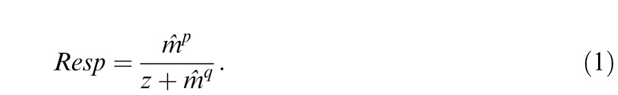Figure 19.

(A) The DSKL model with added binocular contrast gain control after binocular combination. (B) Model simulation of contrast discrimination at a spatial frequency of 0.68 cpd when (1) both test and pedestal are in the DE (dashed blue); (2) both test and pedestal are in the NDE (dashed red); (3) test is in the DE but pedestal is in the NDE (solid blue); (4) test is in the NDE but pedestal is in the DE (solid red); (5) test and pedestal are in both eyes (solid black). Model parameters for DSKL come from the preceding article for normal observer KT and from Table 2 for observers GD, GJ, and PB, and the parameters for binocular contrast gain control are from Meese et al. (2006) with p = 2.76, q = 2.34, z = 4.59, and σ = 0.212. (C) Attenuation effect from model simulation of contrast discrimination when attenuation is fixed at 0.25 for all four observers. Other model parameters are the same as in (B).

We simulate the combined model for each of our individual observers using the parameters of the DSKL model that best fit both the phase and contrast binocular combination data (Table A1 for abnormal observers and see preceding article for normal observers) plus the parameters of the monocular gain control from Meese et al. (2006) that best fit their monocular contrast discrimination data for their normal observers.

The simulation of monocular contrast discrimination for a normal observer (KT, top left in Figure 19B) is identical to the one that used the same parameters of monocular gain control in Meese et al. (2006) because the DSKL model doesn't affect monocular contrast perception. The two monocular threshold-pedestal curves (dashed curves) are overlapped with each other for normal observer KT. However, for abnormal observers who have attenuation in the NDE (three are shown in Figure 19B), the NDE threshold is slightly elevated at low pedestal contrasts (dashed red), but the two monocular curves (dashed red and blue) are almost parallel, inconsistent with the observation of less facilitation in the NDE than in the DE seen in previous studies (Baker et al., 2008; Harrad & Hess, 1992; Levi et al., 1980; Levi, Harwerth, & Smith, 1979). Therefore, attenuation in the NDE alone is not sufficient to account for monocular contrast discrimination in anomalous binocular vision. Baker et al. (2008) proposed a model which added multiplicative noise to the NDE before binocular combination to explain their data. An alternative solution would be to add two different monocular gain controls to the DE and NDE, respectively, before binocular combination. After fitting the two monocular gain controls separately, we can combine them with the DSKL model to predict dichoptic and binocular masking data. Because the DSKL model has no effect on monocular vision, the combined model would give the same predictions for monocular masking as the two separate monocular gain controls. However, as noted by Baker et al. (2008), changing gain parameters is not equivalent to adjusting saturation constant. In the alternative solution, we still need to test if adding noise to the NDE would further improve the model performance.

The simulation of dichoptic contrast discrimination for a normal observer (KT—solid blue and red curves, top-left in Figure 19B) provides reasonable predictions, showing reduced facilitation at low contrasts and stronger masking at high contrasts than observed for monocular masking, similar to the data of Meese et al. (2006). For abnormal observers, the simulation predicts asymmetric dichoptic masking, less facilitation, and stronger masking when testing the NDE (solid red) compared to the DE (solid blue), consistent with observations from Harrad and Hess (1992) and Levi, Harweth, and Smith (1979, 1980). However, simulation of the two-stage model (Baker et al., 2008) results in similar dichoptic masking in the two eyes even when the gain-control weights differ by a factor of 10; unlike the DSKL model, the asymmetric gain controls in the first stage of the two-stage model failed to account for the asymmetry in dichoptic masking.

Simulation of binocular contrast discrimination (solid black curves) predicts the expected binocular advantage at low pedestal contrasts for a normal observer (KT). The predicted binocular summation index (bino/mono) is near two, i.e., full summation at the lowest contrast and then decreases when pedestal contrast increases to the point (the intersection of the black curve and the dashed curve) of no binocular advantage (bino/mono = one). Further increasing pedestal contrast, binocular inhibition (bino/mono < one) appears over a contrast range, and then the monocular (red dashed) and binocular (solid black) curves are quite similar at high pedestal contrast (bino/mono = one).

For normal vision, the binocular advantage is well documented. However, the degree of the advantage in the literature varies substantially, dependent on both the visual stimuli and tasks. Typically, at detection threshold, contrast sensitivity is ≈1.4 to nearly two times higher in binocular vision than in monocular vision (Anderson & Movshon, 1989; Campbell & Green, 1965; Legge, 1984; Meese et al., 2006; Simmons, 2005). However, in contrast matching or contrast discrimination tasks, no binocular advantage is observed at high contrast levels (Legge, 1984; Legge & Rubin, 1981; Meese et al., 2006). For anomalous binocular vision, binocular inhibition (bino/mono < one) has been reported in measures of reaction time (Levi, Harwerth, & Manny, 1979) and contrast sensitivity (Hood & Morrison, 2002; Pardhan & Gilchrist, 1992). Pardhan and Gilchrist (1992) reported that the binocular ratio, bino/mono, depended on the difference between the DE and NDE; minimal interocular difference produced binocular summation and high interocular asymmetry produced binocular inhibition, which is consistent with our simulation and with data of Baker, Meese, Mansouri, and Hess (2007). For observer PB who has high asymmetry across the two eyes (see Figure 2), the predicted binocular inhibition is stronger in magnitude and could be observed over a wider range of pedestal contrast in the simulation (bottom-right in Figure 19B).

In order to study the effect of the contrast attenuation in the NDE on contrast discrimination, we simulate the DSKL model using the fitted parameters, except for attenuation which was fixed at 0.25 for all four observers (Figure 19C). For monocular discrimination, decreasing attenuation in the NDE (or RE) results in parallel shifts of the TvC curve upward and rightward, with no effect on the facilitation dip and masking slope. However, for dichoptic masking, decreasing attenuation in the NDE (or RE) results in reduced facilitation and a shallower masking slope in both eyes. For binocular contrast discrimination, the binocular advantage at low contrast almost disappears and masking behavior at high contrast becomes more similar to that in the DE. These simulated results are qualitatively similar to the data of Baker et al. (2008) (their figure 9).

Implications for normal vision

The interocular enhancement revealed by studying binocular combination in anomalous binocular vision might play an important role in understanding both normal and abnormal binocular vision. This interocular enhancement is not easily evident in normal vision. Observers with abnormal binocular vision may, like dichromats in color vision, place additional constraints on the models and provide new insight into the nature of binocular interaction. Through balancing inhibition and enhancement across the two eyes, the normal visual system achieves constant binocular vision over a large range of variance in visual inputs under normal viewing condition. Losing this delicate balance results in abnormal binocular vision, as occurs in the case of amblyopic vision, and recovering the balance might provide useful new treatments for amblyopic vision.

Appendix: Modeling details

Introduction

In the preceding article (Ding, Klein, & Levi, 2013), we proposed and compared five models with symmetric model parameters in the two eyes to account for normal binocular combination. Here we have modified these models to allow asymmetric parameters between the two eyes in order to account for binocular combination in abnormal binocular vision and amblyopia.

Model 1: Contrast weighted summation model, including asymmetric contrast sensitivity

This model is the Ding-Sperling model with asymmetric contrast sensitivities of the two eyes. It assumes that the interocular gain controls are symmetric. Let I_d and I_n be inputs to DE and NDE, respectively, and μ be the attenuation in NDE. The Ding-Sperling model is given by

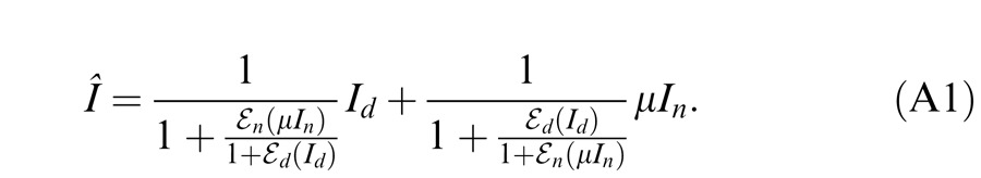With the assumption of symmetric gain control, the contrast energies in both eyes are given by E_d = (m_d/g_c)^γ and E_n = (μm_n/g_c)^γ, using the same gain-control threshold g_c and exponent γ to calculate the two eyes contrast energies. However, the NDE would give less suppression to DE because of lower contrast sensitivity in the NDE. When g_c is small enough, Equation A1 is simplified to be

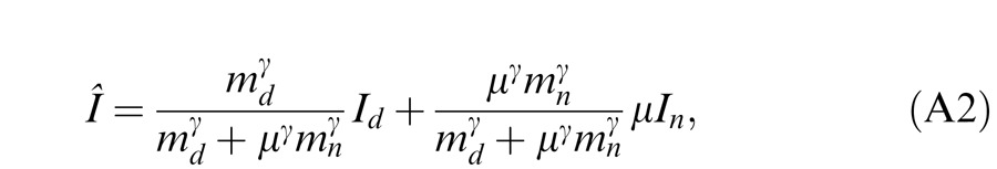a simplified Ding-Sperling model or contrast-weighted summation model. The model has two parameters for one spatial frequency, an attenuation coefficient (μ) in the signal path of NDE, and a gamma exponent (γ) for contrast energy calculation in a control path, and four parameters for three spatial frequencies, one attenuation coefficient for each frequency channel, and one gamma exponent shared by all three frequency channels.

Table A1.

DSKL model parameters for the best fits.

	sf (cpd)	μ	gcd	gcn	αd	αn	γd	γn	ged/gcd	gen/gcn	βd	βn	${\gamma }_d^{*}$	${\gamma }_n^{*}$	gf	γf
GJ	0.68	0.8 ± 0.03	0.062 ± 0.007	0.060 ±0.02	1.04 ± 0.32	0.16 ± 0.07	2.60 ± 0.14	1.62 ± 0.21	2.11 ± 0.27	1.50 ± 0.20	1.0 ± 0.28	0.31 ± 0.17	2.92 ± 0.18	2.23 ± 0.18	0.41 ± 0.20	1
	1.36	0.92 ± 0.05	0.032 ± 0.003	0.107 ±0.042					2.43 ± 0.28	0.78 ± 0.13
	2.72	1.09 ± 0.06	0.022 ± 0.003	0.138 ± 0.067					3.87 ± 0.74	0.40 ± 0.09
GD	0.68	0.93 ± 0.01	0.0043 ± 0.002	0.011 ± 0.005	0.29 ± 0.06	1.85 ± 0.54	2.23 ± 0.09	1.93 ± 0.11	1.30 ± 0.41	2.07 ± 0.24	0.21 ± 0.04	0.97 ± 0.35	1.37 ± 0.17	2.14 ± 0.10	0.005 ± 0.004	0.14 ± 0.08
	1.36	0.95 ± 0.02	0.019 ± 0.003	0.13 ± 0.02					2.42 ± 0.47	1.04 ± 0.06					0.05 ± 0.03
	2.72	0.90 ± 0.02	0.014 ± 0.002	0.15 ± 0.04					7.60 ± 6.50	0.77 ± 0.07
AB	0.68	1.0 ± 0.05	0.032 ± 0.004	0.057 ±0.022	0.21 ± 0.02	0.21 ± 0.02	3.63 ± 0.42	2.01 ± 0.31	1.87 ± 0.18	1.58 ± 0.35	0.31 ± 0.03	0.31 ± 0.03	4.29 ± 0.40	3.33 ± 0.35
BK	0.68	0.87 ± 0.04	0.034 ± 0.004	0.068 ± 0.009	0.49 ± 0.03	0.49 ± 0.03	5.86 ± 1.05	5.90 ± 1.03	1.71 ± 0.18	1.87 ± 0.25	0.36 ± 0.054	0.52 ± 0.05	7.18 ± 1.04	7.15 ± 1.08
PB	0.68	0.86 ± 0.03	0.017 ± 0.003	0.039 ± 0.017	0.15 ± 0.01	0.15 ± 0.01	2.51 ± 0.18	1.19 ± 0.16	4.31 ± 0.47	5.97 ± 2.30	0.35 ± 0.04	0.35 ± 0.04	3.97 ± 0.27	6.55 ± 0.73
MY	0.68	0.74 ± 0.03	0.107 ± 0.019	0.329 ± 0.349	0.5	0.5	5.10 ± 1.18	1.20 ± 3.37	4	2.00 ± 2.32	0.13	0.13	8.34 ± 3.38	8.34 ± 3.38

Table A2.

Statistics for model comparisons. Notes: v: Number of the degrees of freedom. χ²: The weighted sum of squared errors between model predictions and real data. F test: a statistic test comparing the variance between two models with the variance inside the second model, the test value is shown in the row of the second model.

	GJ			GD			BK			AB			PB			MY
	v	χ 2	F test	v	χ 2	F test	v	χ 2	F test	v	χ 2	F test	v	χ 2	F test	v	χ 2	F test
Model 1	247	29335		611	75913		90	1111		46	5174		35	8780		35	2433
Model 2	240	7407	101	604	20531	233	87	593	25.3	43	1880	25.1	32	3548	15.7	32	523	38.9
Model 3a	238	7325	1.34	602	10436	291	85	471	11	41	1307	9	30	519	87.5	30	450	2.4
Model 3b	230	2523	54.7	594	2321	260	81	223	22.6	37	209	57.2	26	189	11.3	30	48	Inf
DSKL model	228	606	361	592	1700	108	80	121	66.7	37	44	Inf	26	20	Inf	30	48	–

As shown in Figure 9A and Table A2, including only asymmetric contrast perception is not enough to account for the asymmetry in binocular combination in amblyopic vision.

Model 2: Ding-Sperling model including asymmetric gain-control parameters

Adding asymmetric gain-control parameters to the Ding-Sperling model significantly improves model fitting (Table A2). The model output is still given by Equation A1, but gain-control contrast energies are given by

with different gain-control thresholds (g_cd and g_cn) and exponents (γ_d and γ_n) in the two eyes. Because the NDE-to-DE suppression might be weak or even absent, i.e., the NDE has a high gain-control threshold g_cn, the constant term ‘1’ in Equation A1 has to be considered in the calculation, and the model cannot be simplified. Model 2 has five parameters for each frequency channel, one attenuation coefficient μ, two gain-control thresholds g_cd and g_cn, and two gain-control exponents γ_d and γ_n. With sharing two gain-control exponents across spatial frequency channels, the model has 11 parameters for three frequency channels. As shown in Figure 9B, when required to share constraints with each other, the perceived phase and contrast cannot be accounted for simultaneously by asymmetries in contrast sensitivity and in interocular contrast gain control.

Model 3a: Adding asymmetry between gain controls of the two layers

Model 3a adds relative gain-control efficiency α in the second layer gain control (the blue layer in Figure 10) when the gain-control efficiency in the signal layer (the black layer in Figure 10) is assumed to be one. For amblyopic vision, there are different model parameters for the two eyes, α_d for DE and α_n for NDE, which are assumed to be shared across spatial frequency channels. Model 3a has seven parameters for one frequency channel and 13 parameters for three frequency channels. Its output is given by

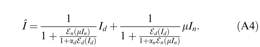However, although it significantly improved data fitting (Table A2), adding asymmetry between gain controls of the two layers is still not able to solve the contradiction in accounting for the perceived phase and contrast from the model; like Model 2, Model 3a predicts weaker DE-to-NDE inhibition than the actual phase data showed but stronger DE-to-NDE inhibition than the actual contrast data demonstrated.

Model 3b: Adding interocular contrast enhancement

The model output is given by

$E_n^{*}$ and $E_d^{*}$ are gain-enhancement contrast energies in DE and NDE, respectively, given by

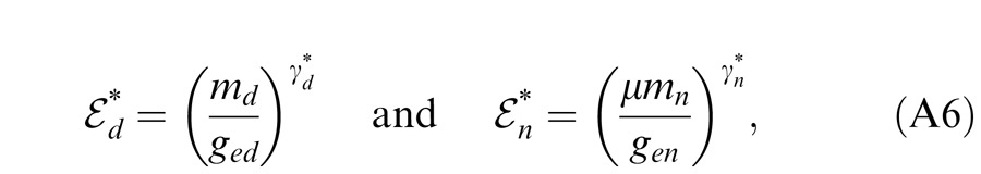where g_ed and g_en are gain-enhancement thresholds, and ${\gamma }_d^{*}$ and ${\gamma }_n^{*}$ are gain-enhancement exponents. By adding gain-enhancement parameters, Model 3b has 11 parameters for one spatial frequency channel and 21 parameters for three spatial frequency channels. As shown in Figure 9C, adding interocular contrast enhancement is helpful to solve the contradiction when fitting the Ding-Sperling model to both phase and contrast data (Figure 9B), significantly improving model fitting. NDE-to-DE enhancement makes the perceived phase further shift to the DE when the NDE's contrast (base contrast) increases to 48% and 96% while DE-to-NDE enhancement balances DE-to-NDE inhibition in the perceived contrast contour when the DE's contrast increases from zero to a small value making apparent inhibition less than predicted from the Ding-Sperling model and, therefore, better fitting the real data. However, at higher spatial frequencies (Figures 9D and E), more interocular asymmetry could be observed in both phase and contrast data. The fits from Model 3b show a new contradiction in the prediction of contrast contour; the apparent inhibition from the model is much stronger than the real data at 24% equal contrast contour (red), while it is much weaker than the real data at 48% equal contrast contour (blue). The DE-to-NDE enhancement is less than needed to balance the DE-to-NDE inhibition at 24% contrast, while it is more than needed at 48% contrast. To solve this contradiction, this DE-to-NDE enhancement should be controlled by NDE's contrast.

The DSKL model (Model 3c): Adding mutual inhibition to interocular contrast enhancement

The model output is given by

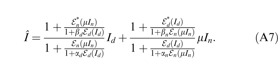By adding the gain control of the gain enhancement, the DSKL model (Figure 10) significantly improves model fits (Figures 2–8) even though only two model parameters, relative gain-control efficiency β_d and β_n, are added to the Model 3b.

Table A3.

Comparison with MCM. Notes: v: Number of the degrees of freedom. χ²: The weighted sum of squared errors between model predictions and real data. AIC: Akaike information criterion.

	GJ (0.68 cpd)			GJ (1.36 cpd)			GJ (2.72 cpd)			GD (0.68 cpd)			GD (1.36 cpd)
	v	χ2/v	AIC	v	χ2/v	AIC	v	χ2/v	AIC	v	χ2/v	AIC	v	χ2/v	AIC
Model 1	89	63.7	5675	87	124.8	10865	59	216	12762	106	44.8	4748	238	175	41550
Model 2	86	13.3	1157	84	30.2	2544	56	72.5	4071	103	9	942	235	43	10104
MCM	85	7.1	619	83	17.3	1450	55	29	1604	102	3.3	352	234	10.9	2574
Model 3a	84	9.7	825	82	28.3	2330	54	68.7	3723	101	2.2	241	233	19.7	4610
Model 3b	80	4.1	351	78	6.6	535	50	27.1	1377	97	2	215	229	3.1	734
DSKL model	78	2	178	76	1.8	161	48	2.4	139	95	1.6	177	227	2.2	535

Table A3.

Extended.

	GD (2.72 cpd)			BK (0.68 cpd)			AB (0.68 cpd)			PB (0.68 cpd)			MY (0.68 cpd)
	v	χ2/v	AIC	v	χ2/v	AIC	v	χ2/v	AIC	v	χ2/v	AIC	v	χ2/v	AIC
Model 1	99	111.3	11025	90	12.3	1115	46	112.5	5178	35	251	8784	35	69.5	2437
Model 2	96	33.3	3209	87	6.8	603	43	43.7	1890	32	111	3558	32	16.4	533
MCM	95	5.3	513	86	6.4	560	42	21.6	920	31	39.1	1224	31	11.9	381
Model 3a	94	21.7	2056	85	5.5	485	41	31.9	1321	30	17.3	533	30	15	464
Model 3b	90	4.5	431	81	2.7	245	37	5.6	231	26	7.3	211	30	1.6	62
DSKL model	88	2.8	270	80	1.5	145	37	1.2	66	26	0.8	42	30	1.6	62

In the DSKL model, one eye's three gain controls in the signal layer (black), gain-control layer (blue), and gain-enhancement layer (red) receive gain controls from the other eye's gain-control layer. The model has 13 parameters for one spatial frequency channel and 23 parameters for three spatial frequency channels. Table A1 shows the model parameters for the best fits that are displayed in Figures 2–8. For observer MY, because data are not sufficient to fit all model parameters, we fixed some model parameters to the average values for normal observers (see preceding article).

Table A2 shows statistics for comparison of five models for all observers. Except for observer MY, for each step of modification, the fitting error chi-squared is significantly improved and an F test, a statistic test comparing the variance between models with the variance inside model, shows that the previous model could be rejected with a very small probability (<0.001) of false of rejection. For observer MY, because some model parameters in Models 3b and the DSKL model were fixed, the number of the degree of freedom (v) of these models was the same as in Model 3a. However, after including interocular enhancement, Model 3b significantly improved data fitting comparing with Model 3a even without decreasing degrees of freedom (v) of the model. Table A3 shows statistics for comparison of our five models with MCM.

References

- Agrawal R., Conner I. P., Odom J. V., Schwartz T. L., Mendola J. D. (2006). Relating binocular and monocular vision in strabismic and anisometropic amblyopia. Archives of Ophthalmology , 124 (6), 844– 850. [DOI] [PubMed] [Google Scholar]
- Anderson P. A., Movshon J. A. (1989). Binocular combination of contrast signals. Vision Research , 29 (9), 1115– 1132. [DOI] [PubMed] [Google Scholar]
- Baker D. H., Meese T. S., Hess R. F. (2008). Contrast masking in strabismic amblyopia: Attenuation, noise, interocular suppression and binocular summation. Vision Research , 48 (15), 1625– 1640. [DOI] [PubMed] [Google Scholar]
- Baker D. H., Meese T. S., Mansouri B., Hess R. F. (2007). Binocular summation of contrast remains intact in strabismic amblyopia. Investigative Ophthalmology & Visual Science , 48 (11), 5332– 5338, http://www.iovs.org/content/48/11/5332 [PubMed] [Article] [DOI] [PubMed] [Google Scholar]
- Baker D. H., Wallis S. A., Georgeson M. A., Meese T. S. (2012). The effect of interocular phase difference on perceived contrast. PLoS One, 7 (4), 14. [DOI] [PMC free article] [PubMed] [Google Scholar]
- Bi H., Zhang B., Tao X., Harwerth R. S., Smith E. L., Chino Y. M. (2011). Neuronal responses in visual area V2 (V2) of macaque monkeys with strabismic amblyopia. Cerebral Cortex , 21 (9), 2033– 2045. [DOI] [PMC free article] [PubMed] [Google Scholar]
- Campbell F. W., Green D. G. (1965). Monocular versus binocular visual acuity. Nature , 208 (5006), 191– 192. [DOI] [PubMed] [Google Scholar]
- Chino Y. M., Smith E. L., III, Hatta S., Cheng H. (1997). Postnatal development of binocular disparity sensitivity in neurons of the primate visual cortex. The Journal of Neuroscience , 17 (1), 296– 307. [DOI] [PMC free article] [PubMed] [Google Scholar]
- Ding J., Klein S., Levi D. (2009). Binocular combination in amblyopic vision. Journal of Vision , 9 (8): 14 http://www.journalofvision.org/content/9/8/274, doi:10.1167/9.8.274 [Abstract] [DOI] [PMC free article] [PubMed] [Google Scholar]
- Ding J., Klein S., Levi D. (2013). Binocular combination of phase and contrast explained by a gain-control and gain-enhancement model. Journal of Vision , 13 (2): 14, 1– 37, http://www.journalofvision.org/content/13/2/13, doi:10.1167/13.2.13. [DOI] [PMC free article] [PubMed] [Google Scholar]
- Ding J., Levi D. M. (2011). Recovery of stereopsis through perceptual learning in human adults with abnormal binocular vision. Proceedings of the National Academy of Sciences of the USA , 108 (37), E733– E741. [DOI] [PMC free article] [PubMed] [Google Scholar]
- Ding J., Sperling G. (2006). A gain-control theory of binocular combination. Proceedings of the National Academy of Sciences of the USA , 103 (4), 1141– 1146. [DOI] [PMC free article] [PubMed] [Google Scholar]
- Ding J., Sperling G. (2007). Binocular combination: Measurements and a model. In Harris L., Jenkin M. (Eds.), Computational vision in neural and machine systems ( pp 257– 305). Cambridge, UK: Cambridge University Press. [Google Scholar]
- Foley J. M., Legge G. E. (1981). Contrast detection and near-threshold discrimination in human vision. Vision Research , 21 (7), 1041– 1053. [DOI] [PubMed] [Google Scholar]
- Freeman R., Ohzawa I. (1992). Development of binocular vision in the kitten's striate cortex. The Journal of Neuroscience , 12 (12), 4721– 4736. [DOI] [PMC free article] [PubMed] [Google Scholar]
- Goodman L. K., Black J. M., Phillips G., Hess R. F., Thompson B. (2011). Excitatory binocular interactions in two cases of alternating strabismus. Journal of American Association for Pediatric Ophthalmology and Strabismus, 15 (4), 345– 349. [DOI] [PubMed] [Google Scholar]
- Harrad R. A., Hess R. F. (1992). Binocular integration of contrast information in amblyopia. Vision Research , 32 (11), 2135– 2150. [DOI] [PubMed] [Google Scholar]
- Harrad R. A., Sengpiel F., Blakemore C. (1996). Physiology of suppression in strabismic amblyopia. British Journal of Ophthalmology , 80 (4), 373– 377. [DOI] [PMC free article] [PubMed] [Google Scholar]
- Harwerth R. S., Levi D. M. (1983). Psychophysical studies on the binocular processes of amblyopes. American Journal of Optometry and Physiological Optics, 60 (6), 454– 463. [DOI] [PubMed] [Google Scholar]
- Hess R. F., Bradley A. (1980). Contrast perception above threshold is only minimally impaired in human amblyopia. Nature, 287 (5781), 463– 464. [DOI] [PubMed] [Google Scholar]
- Holopigian K., Blake R., Greenwald M. J. (1988). Clinical suppression and amblyopia. Investigative Ophthalmology & Visual Science , 29 (3), 444– 451, http://www.iovs.org/content/29/3/444 [PubMed] [Article] [PubMed] [Google Scholar]
- Hood A. S., Morrison J. D. (2002). The dependence of binocular contrast sensitivities on binocular single vision in normal and amblyopic human subjects. The Journal of Physiology, 540 (2), 607– 622. [DOI] [PMC free article] [PubMed] [Google Scholar]
- Horton J. C., Hocking D. R. (1996). Intrinsic variability of ocular dominance column periodicity in normal macaque monkeys. The Journal of Neuroscience , 16 (22), 7228– 7339. [DOI] [PMC free article] [PubMed] [Google Scholar]
- Hou F., Huang C. B., Zhou Y. F., Lu Z. L. (2012). Contrast gain control in stereo depth and cyclopean contrast perception. Journal of Vision , 12 (9): 14 http://www.journalofvision.org/content/12/9/45, doi:10.1167/12.9.45 [Abstract] [DOI] [PMC free article] [PubMed] [Google Scholar]
- Huang C. B., Zhou J., Lu Z. L., Feng L., Zhou Y. (2009). Binocular combination in anisometropic amblyopia. Journal of Vision , 9 (3): 14 11– 16, http://www.journalofvision.org/content/9/3/17, doi:10.1167/9.3.17 [PubMed] [Article] [DOI] [PMC free article] [PubMed] [Google Scholar]
- Huang C. B., Zhou J., Lu Z. L., Zhou Y. (2011). Deficient binocular combination reveals mechanisms of anisometropic amblyopia: Signal attenuation and interocular inhibition. Journal of Vision , 11 (6): 14 1– 17, http://www.journalofvision.org/content/11/6/4, doi:10.1167/11.6.4 [PubMed] [Article] [DOI] [PMC free article] [PubMed] [Google Scholar]
- Huang C. B., Zhou J., Zhou Y., Lu Z. L. (2010). Contrast and phase combination in binocular vision. PLoS One, 5 (12), e15075. [DOI] [PMC free article] [PubMed] [Google Scholar]
- Legge G. E. (1981). A power law for contrast discrimination. Vision Research , 21 (4), 457– 467. [DOI] [PubMed] [Google Scholar]
- Legge G. E. (1984). Binocular contrast summation--I. Detection and discrimination. Vision Research , 24 (4), 373– 383. [DOI] [PubMed] [Google Scholar]
- Legge G. E., Gu Y. C. (1989). Stereopsis and contrast. Vision Research , 29 (8), 989– 1004. [DOI] [PubMed] [Google Scholar]
- Legge G. E., Rubin G. S. (1981). Binocular interactions in suprathreshold contrast perception. Perception & Psychophysics , 30 (1), 49– 61. [DOI] [PubMed] [Google Scholar]
- Lema S. A., Blake R. (1977). Binocular summation in normal and stereoblind humans. Vision Research , 17 (6), 691– 695. [DOI] [PubMed] [Google Scholar]
- Levi D. M., Harwerth R. S., Manny R. E. (1979). Suprathreshold spatial frequency detection and binocular interaction in strabismic and anisometropic amblyopia. Investigative Ophthalmology & Visual Science , 18 (7), 714– 725, http://www.iovs.org/content/18/7/714 [PubMed] [Article] [PubMed] [Google Scholar]
- Levi D. M., Harwerth R. S., Smith E. L. (1980). Binocular interactions in normal and anomalous binocular vision. Documenta Ophthalmologica , 49 (2), 303– 324. [DOI] [PubMed] [Google Scholar]
- Levi D. M., Harwerth R. S., Smith E. L., III. (1979). Humans deprived of normal binocular vision have binocular interactions tuned to size and orientation. Science, 206 (4420), 852– 854. [DOI] [PubMed] [Google Scholar]
- Li J., Thompson B., Lam C. S. Y., Deng D., Chan L. Y. L., Maehara G., et al. (2011). The role of suppression in amblyopia. Investigative Ophthalmology & Visual Science , 52 (7), 4169– 4176, http://www.iovs.org/content/52/7/4169 [PubMed] [Article] [DOI] [PubMed] [Google Scholar]
- Loshin D., Levi D. (1983). Suprathreshold contrast perception in functional amblyopia. Documenta Ophthalmologica, 55 (3), 213– 236. [DOI] [PubMed] [Google Scholar]
- McKee S. P., Levi D. M., Movshon J. A. (2003). The pattern of visual deficits in amblyopia. Journal of Vision , 3 (5): 14 380– 405, http://www.journalofvision.org/content/3/5/5, doi:10.1167/3.5.5 [PubMed] [Article] [DOI] [PubMed] [Google Scholar]
- Meese T. S., Georgeson M. A., Baker D. H. (2006). Binocular contrast vision at and above threshold. Journal of Vision , 6 (11): 14 1224– 1243, http://www.journalofvision.org/content/6/11/7, doi:10.1167/6.11.7 [PubMed] [Article] [DOI] [PubMed] [Google Scholar]
- Pardhan S., Gilchrist J. (1992). Binocular contrast summation and inhibition in amblyopia. The influence of the interocular difference on binocular contrast sensitivity. Documenta Ophthalmologica , 82 (3), 239– 248. [DOI] [PubMed] [Google Scholar]
- Simmons D. R. (2005). The binocular combination of chromatic contrast. Perception, 34 (8), 1035– 1042. [DOI] [PubMed] [Google Scholar]
- Smith E. L., Chino Y. M., Ni J., Cheng H., Crawford M. L. J., Harwerth R. S. (1997). Residual binocular interactions in the striate cortex of monkeys reared with abnormal binocular vision. Journal of Neurophysiology , 78 (3), 1353– 1362. [DOI] [PubMed] [Google Scholar]
- Stelmach L. B., Tam W. J. (1996, January). Stereo-anomalous vision in a sample of young adults. Paper presented at the Proceedings of SPIE, San Jose, California. [Google Scholar]