

Abstract
The MemToolbox is a collection of MATLAB functions for modeling visual working memory. In support of its goal to provide a full suite of data analysis tools, the toolbox includes implementations of popular models of visual working memory, real and simulated data sets, Bayesian and maximum likelihood estimation procedures for fitting models to data, visualizations of data and fit, validation routines, model comparison metrics, and experiment scripts. The MemToolbox is released under the permissive BSD license and is available at http://memtoolbox.org.
Keywords: visual working memory, mixture models, model comparison
Introduction
Working memory is a storage system that actively holds information in mind and allows for its manipulation, providing a workspace for thought (Baddeley, 1986). Its strikingly limited capacity has inspired a slew of research aimed at characterizing those limits in terms of the spatiotemporal properties of the stimulus and the age, intelligence, tiredness, and mental health of the individual.
A handful of experimental paradigms predominate the study of working memory. These include the delayed match-to-sample task used in studies of animal cognition (Blough, 1959) and the span tasks used in studies of verbal working memory (Daneman & Carpenter, 1980). Research on visual working memory relies primarily on two tasks: partial report and change detection (Figure 1). In a partial-report task, the participant is shown a set of letters, shapes, or colorful dots and then after a brief delay is asked to report the properties of one or a subset of the items (Sperling, 1960; Wilken & Ma, 2004; Zhang & Luck, 2008). In a change-detection task, the participant is shown a pair of displays, one after the other, and is asked a question that requires comparing them, such as whether they match (Phillips, 1974; Pashler, 1988; Luck & Vogel, 1997).
Figure 1.
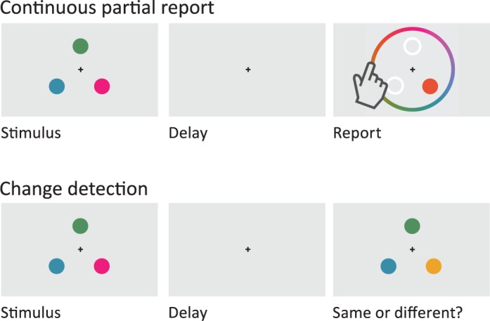
(top) A continuous partial-report task. The observer sees the stimulus display and then after a delay is asked to report the exact color of a single item. (bottom) A change-detection task. The observer sees the stimulus display and then after a delay is asked to report whether the test display matches.
Formal models have been proposed that link performance in change-detection and partial-report tasks to the architecture and capacity of the working-memory system. These include the item-limit model (Pashler, 1988), the slot model (Luck & Vogel, 1997; Cowan, 2001), the slots + averaging model (Figure 2; Zhang & Luck, 2008), the slots + resources model (Awh, Barton, & Vogel, 2007), the continuous-resource model (Wilken & Ma, 2004), the resources + swaps model (Bays, Catalao, & Husain, 2009), the ensemble statistics + items model (Brady & Alvarez, 2011), and the variable-precision model (Fougnie, Suchow, & Alvarez, 2012; van den Berg, Shin, Chou, George, & Ma, 2012;). Each model specifies the structure of visual memory and the decision process used to perform the task.
Figure 2.
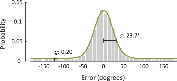
An example of a model's fit to continuous partial-report data. Most responses fall within a relatively small range around the target item's true value, but some responses are far off. The data are fit using the mixture model of Zhang and Luck (2008), which attributes the gap in performance to differences in the state of memory for the target item: With probability g, the observer remembers nothing about the item and guesses randomly; with probability 1 − g, the observer has a noisy representation of the item, leading to responses centered at the true value and with a standard deviation σ that reflects the quality of the observer's memory.
Having been fit to the data, these models are used to make claims about the architecture and capacity of memory. For example, using an item-limit model to fit data from a change-detection task, Luck and Vogel (1997) showed that observers can remember the same number of objects no matter whether they store one or two features per object (e.g., only color vs. both color and orientation) and from this inferred that the storage format of visual working memory is integrated objects, not individual features. Using data from a continuous partial-report task, Brady and Alvarez (2011) showed that when items are presented in a group, memory for an individual item is biased toward the group average and from this inferred that working memory is hierarchical, representing both ensembles of items and individual items.
The MemToolbox
We created the MemToolbox, a collection of MATLAB functions for modeling visual working memory. The toolbox provides everything needed to perform the analyses commonly used in studies of visual working memory, including model implementations, maximum likelihood routines, and data validation checks, although it defaults to a Bayesian workflow that encourages a deeper look into the data and the models' fits. In the following sections, we highlight the toolbox's core functionality and describe the improvements it offers to the standard workflow. We begin by reviewing the standard workflow and its implementation in the toolbox.
The standard workflow
The experimenter first picks a model. Then, to fit the model to experimental data using probabilistic methods, a likelihood function is defined that describes the model's predictions for each possible setting of its parameters. (Formally, given a model M with free parameters θ, the model's likelihood function specifies a probability distribution P(D|θ) over possible datasets D.) With the likelihood function in hand, an estimator is used to pick the parameter settings that provide the best fit to the data. A popular choice is the maximum likelihood estimator, which selects the parameter values that maximize the model's likelihood function given the data (Dempster, Laird, & Rubin, 1977; Lagarias, Reeds, Wright, & Wright, 1998). Typically, this procedure is performed separately for each participant and experimental condition, resulting in parameter estimates that are then compared using traditional statistical tests (e.g., Zhang & Luck, 2008).
The MemToolbox uses two MATLAB structures (“structs'') to organize the information needed to analyze data using the standard workflow: one that describes the data to be fit and another that describes the model and its likelihood function.
Fitting a set of data with a model is then as simple as calling the built-in MLE() function. For example, if data was obtained from a continuous color-report task in which an observer made errors of −89°, 29°, etc., a model could be fit using the following workflow:
>> model = StandardMixtureModel();
>> data.errors = [-89,29,-2,6,-16,65,43,-12,10,0,178,-42];
>> fit = MLE(data, model)
This will return the maximum likelihood parameters for this observer's data, allowing for standard analysis techniques to be used.
Thus, with little effort, the MemToolbox can be used to simplify (and speed up) existing workflows by allowing for straightforward fitting of nearly all the standard models used in the visual working-memory literature. In support of this goal, the toolbox includes descriptive models, such as the StandardMixtureModel (that of Zhang & Luck, 2008) and SwapModel of Bays et al. (2009), as well as several explanatory models, such as VariablePrecisionModel (e.g., Fougnie et al., 2012; van den Berg et al., 2012). For more information about a particular model m, type help m at the MATLAB prompt. For example, to access the help file for StandardMixtureModel, run help StandardMixtureModel. It is also possible to view the full code for a model by running edit m. (In fact, this applies to any function in the toolbox.) For example, to view the code for the swap model, type edit SwapModel, which will show the model's probability distribution function, the parameter ranges, and the specification of priors for the model parameters.
The toolbox also includes a number of wrapper functions that extend existing models and make them more robust. For example, the wrapper function WithBias() adds a bias term, WithLapses() adds an inattention parameter, and Orientation() alters a model so that it uses a 180° error space, appropriate for objects that are rotationally symmetric, e.g., line segments. Inattention parameters are particularly important because deciding whether to include such parameters has an inordinate influence on parameter estimation and model selection (Rouder et al., 2008). Many of the standard models in the toolbox (e.g., StandardMixtureModel) already include such inattention parameters.
The Bayesian workflow
By default, instead of returning the maximum likelihood estimate, the toolbox uses a Bayesian workflow that constructs a full probability distribution over parameter values. This probability distribution describes the reasonableness of each possible parameter setting after considering the observed data in light of prior beliefs. In doing so, it strongly encourages a thorough examination of model fit. The Bayesian workflow is implemented as MemFit, the toolbox's primary fitting function.
>> fit = MemFit(data, model)
Bayesian inference provides a rational rule for updating prior beliefs (“the prior”) based on experimental data. The prior, P(θ), conveys which parameter values are thought to be reasonable, and specifying it can be as straightforward as setting upper and lower bounds (for example, bounding the guess rate between 0 and 1). Analysts add value through judicious selection of priors that faithfully reflect their beliefs. Because a prior can have an arbitrarily large impact on the resulting inference, it is important both to carefully consider which distribution is appropriate and, when communicating results that depend on those inferences, to report exactly the choice that was made. For the purposes of exploratory data analysis, it is common to use a noninformative or weakly informative prior that spreads the probability thinly over a swath of plausible parameter values (e.g., the Jeffreys prior, a class of noninformative priors that are invariant under reparameterization of the model; Jeffreys, 1946; Jaynes, 1968) to avoid an inordinate influence of the prior on inferences.
Once specified, beliefs are then updated (according to Bayes' rule) to take into account the experimental data. Bayes' rule stipulates that after observing data D, the posterior beliefs about the parameters (“the posterior”) are given by
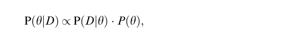 |
which combines the likelihood of the data given the parameters with the prior probability of the parameters.
Estimating the full posterior distribution is harder than finding the maximum likelihood estimate. For some models, it is possible to derive closed-form expressions for the posterior distribution, but for most models, this is intractable, and so sampling-based algorithms are used to approximate it. One such algorithm, the Metropolis-Hastings variant of Markov Chain Monte Carlo (MCMC), is applicable to a wide range of models and is thus the one used by the toolbox (Metropolis, Rosenbluth, Rosenbluth, Teller, & Teller, 1953; Hastings, 1970). The algorithm chooses an initial set of model parameters and then, over many iterations, proposes small moves to these parameter values, accepting or rejecting them based on how probable the new parameter values are in both the prior and the likelihood function. In this way, it constructs a random walk that visits parameter settings with a frequency proportional to their probability under the posterior. This allows the estimation of the full posterior of the model in a reasonable amount of time and is theoretically equivalent to the more straightforward (but much slower) technique of evaluating the model's likelihood and prior at every possible setting of the parameters (implemented in the GridSearch function). For an introduction to MCMC, we recommend Andrieu, De Freitas, Doucet, and Jordan (2003). The MemToolbox includes an implementation of MCMC that attempts, as best as possible, to automate the process of sampling from the posterior of the models that are included in the toolbox.
With the posterior distribution in hand, there are a number of ways to analyze and visualize the results. First, the maximum of the posterior distribution (the maximum a posteriori or MAP estimate) can be used as a point estimate that is analogous to the maximum likelihood estimate, differing only in the MAP's consideration of the prior. (This estimate can be calculated directly using the MAP function). However, visualizing the full posterior distribution also provides information about how well the data constrain the parameter values and whether there are trade-offs between parameters (Figure 3).
Figure 3.
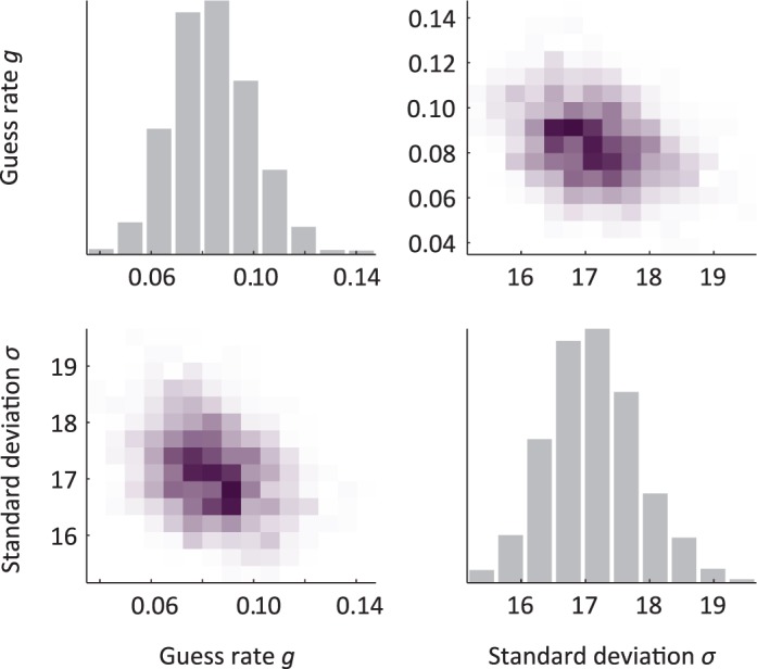
An example of the full posterior of the standard mixture model of Zhang and Luck (2008), where g is the guess rate and sd is the standard deviation of observers' report for remembered items. On the diagonal are plots that show the posterior for an individual parameter, e.g., the distribution for guess rate (g) is plotted in the top left corner. We can see that the data make us quite confident that the guess rate is between 0.05 and 0.12. On the off-diagonals are the correlations between the parameters—for example, the top right axis shows guess rate (y-axis) plotted against standard deviation (x-axis). Each row and each column corresponds to a parameter, e.g., the x-axis for all the plots in the second column corresponds to standard deviation.
Figure 3 shows a posterior distribution for data analyzed with the standard mixture model of Zhang and Luck (2008). The plots on the main diagonal are histograms of values for each parameter, the so-called “marginal” of the posterior distribution; the plots on the off-diagonals reveal correlations between parameters. Note that in the standard-mixture model, there is a slight negative correlation between the standard-deviation parameter and the guess-rate parameter: Data can be seen as having either a slightly higher guess rate and lower standard deviation or a slightly lower guess rate and higher standard deviation. Examining the full posterior reveals this trade-off, which remains hidden when using maximum likelihood fits. This is important when drawing conclusions that depend on how these two parameters relate. For example, Anderson, Vogel, and Awh (2011) found correlations between a measure based on guess rate and another based on standard deviation and used this to argue that each observer has a fixed personal number of discrete memory slots. However, because the parameters trade off, such correlations are meaningful only if the estimates are derived from independent sets of data; otherwise, the correlations are inflated by the noise in estimating the parameters (Brady, Fougnie, & Alvarez, 2011). Thus, understanding the full posterior distribution is critical to correctly estimating parameters and their relationships to each other.
Posterior predictive checks
Another technique applied by the MemToolbox is the automatic use of posterior predictive checks. Sometimes a whole class of models performs poorly, such that there are no parameter settings that will produce a good fit. In this case, maximum likelihood and maximum a posteriori estimates are misleading: They dutifully pick out the best even if the best is still quite bad. A good practice then is to check the quality of the fit, examining which aspects of the data it captures and which aspects it misses (Gelman, Meng, & Stern, 1996; Gelman, Carlin, Stern, & Rubin, 2004). This can be accomplished through a posterior predictive check, which simulates new data from the posterior fit of the model and then compares the histograms of the actual and simulated data (Figure 4). MemFit performs posterior predictive checks by default.
Figure 4.
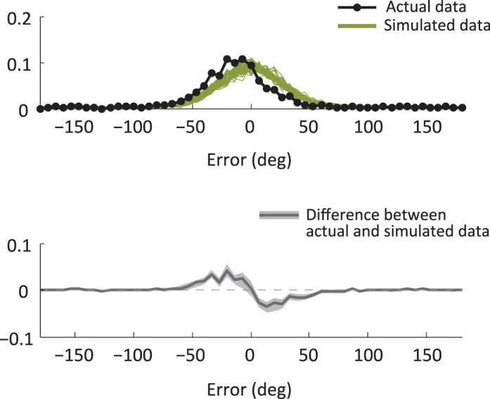
(Top) Simulated data from the posterior of the model (green) with the actual data overlaid (black). The mismatch between the two is symptomatic of a poor fit. (Bottom) The difference between the simulated and real data, bounded by 95% credible intervals. If at any spot the credible interval does not include zero, it is an indication that the model does not accurately fit the data.
A model that can accurately fit the data in a posterior predictive check does not necessarily provide a good fit. For example, the model may fit the averaged data but fail to fit observers' data from individual displays, perhaps because of reports of incorrect items (Bays et al., 2009) or because of the use of grouping or ensemble statistics (Brady & Tenenbaum, 2013). In addition, a good fit does not necessarily indicate a good model: An extremely flexible model that can mimic any data always provides a good fit, but this provides no evidence in favor of that model (Roberts & Pashler, 2000). However, models that systematically deviate in a posterior predictive check nearly always need improvement.
Hierarchical modeling
Typically, the question of interest in working-memory research is not about a single observer, but a population: Do older individuals have reduced working-memory capacity? Do people guess more often when there is more to remember? When aggregating results from multiple participants to answer such questions, the standard technique is to separately fit a model to the data from each participant (using, for example, maximum likelihood estimation) and to combine parameter estimates across participants by taking their average or median. Differences between conditions are then examined through t-tests or ANOVAs. This approach to analyzing data from multiple participants allows generalization to the population as a whole because participant variance is taken into account by treating parameters as random effects (Daw, 2011). One flaw with this approach is that it entirely discards information about the reliability of each participant's parameter estimates. This is particularly problematic when there are differences in how well the data constrain the parameters of each participant (e.g., because of differences in the number of completed trials) or when there are significant trade-offs between parameters (as in the parameters of the standard model), in which case analyzing them separately can be problematic (Brady et al., 2011). For example, the standard deviation parameter of the standard mixture model is considerably less constrained at high guess rates than at low guess rates. Thus, even with the same number of trials, our estimate of the standard deviation will be more reliable for participants with lower guess rates than those with higher guess rates.
A better technique, although one that is more computationally intensive, is to fit a single hierarchical model of all participants (e.g., Rouder, Sun, Speckman, Lu, & Zhou, 2003; Rouder & Lu, 2005; Morey, 2011). This treats each participant's parameters as samples from a normally distributed population and uses the data to infer the population mean and standard deviation of each parameter. This technique automatically gives more weight to participants whose data give more reliable parameter estimates and causes “shrinkage” of each participant's parameter estimates toward the population mean, sensibly avoiding extreme values caused by noisy data. For example, using maximum likelihood estimates, participants with high guess rates are sometimes estimated to have guess rates near zero but standard deviations of 3000° (resulting in a nearly flat normal distribution). This problem is avoided by fitting participants in a hierarchical model.
By default, when given multiple data sets, one per participant, MemFit will separately fit the model to each participant's data. Hierarchical modeling is performed by passing an optional parameter, ‘UseHierarchical’, to MemFit:
>> data1 = MemDataset(1);
>> data2 = MemDataset(2);
>> model = StandardMixtureModel();
>> fit = MemFit({data1,data2}, model, ′UseHierarchical′, true)
Fitting such models is computationally more difficult, and so you should ensure the estimation procedure has correctly converged (e.g., using the PlotConvergence function provided by the toolbox) before relying on the parameter estimates to make inferences.
Model comparison
Which model best describes the data? Answering this question requires considering both the resemblance between the model and the data and also the model's flexibility. Flexible models can fit many data sets, and so a good fit provides only weak evidence of a good match between model and data. In contrast, a good fit between an inflexible model and the data provides stronger evidence of a good match. To account for this, many approaches to model comparison penalize more flexible models; these include the Akaike Information Criterion with correction for finite data (AICC; Akaike, 1974; Burnham & Anderson, 2004), the Bayesian Information Criterion (BIC; Schwarz, 1978), the Deviance Information Criterion (DIC; Spiegelhalter, Best, Carlin, & der Linde, 2002), and the Bayes factor (Kass & Raftery, 1995). It is also possible to perform cross-validation—fitting and testing separate data—to eliminate the advantage of a more flexible model. Implementations of some of these model comparison techniques are provided by the MemToolbox and can be accessed by passing multiple models to the MemFit function:
>> model1 = StandardMixtureModel();
>> model2 = SwapModel();
>> modelComparison = MemFit(data, {model1, model2})
This will output model comparison metrics and describe them, including which model is preferred by each metric.
Despite the array of tools provided by the MemToolbox, we do not wish to give the impression that model selection can be automated. Choosing between competing models is no easier or more straightforward than choosing between competing scientific theories (Pitt & Myung, 2002). Selection criteria such as AICC are simply tools for understanding model fits, and it is important to consider their computational underpinnings when deciding which criterion to use—before performing the analysis. For example, the criteria included in the toolbox are differently calibrated in terms of how strongly they penalize complex models with criteria such as AICC having an inconsistent calibration that penalizes complex models less than criteria such as BIC, which penalizes complex models in a way that depends on their functional form, taking into account correlations between parameters. DIC is the only method appropriate in a hierarchical setting.
In addition to choosing an appropriate model comparison metric, we recommend computing the metric for each participant independently and looking at consistency across participants to make inferences about the best-fitting models. Importantly, by fitting independently for each participant, you can take into account participant variance and are thus able to generalize to the population as a whole (for example, by using an ANOVA over model likelihoods). By contrast, computing a single AICC or BIC value across all participants does not allow generalization to the population as it ignores participant variance; one participant that is fit much better by a particular model can drive the entire AICC or BIC value. This kind of fixed-effects analysis can thus seriously overstate the true significance of results (Stephan et al., 2010). As in the case of estimating parameters, this technique of estimating model likelihoods for each participant and then performing an ANOVA or t-test over these parameters is only an approximation to the fully Bayesian hierarchical model that considers the evidence simultaneously from each participant (Stephan, Penny, Daunizeau, Moran, & Friston, 2009); however, in the case of model comparison, the simpler technique is likely sufficient for most visual working-memory experiments.
To facilitate this kind of analysis, the MemToolbox performs model comparisons on individual participant data, and MemFit calculates many of the relevant model comparison metrics so that you may choose the appropriate comparison for your theoretical claim.
Availability, contents, and help
The MemToolbox is available on the web at http://memtoolbox.org. To install the toolbox, place it somewhere sensible and then run the included Setup.m script, which will add it to MATLAB's default path. The distribution includes source code, demos, and a tutorial that reviews all of the toolbox's functionality. It is released under a BSD license, allowing free use for research or teaching. The organization of the toolbox's folder structure is outlined in the file MemToolbox/Contents.m. Detailed descriptions of each function (e.g., MCMC) can be found in the help sections contained in each file. To access the help section for some function f from the MATLAB prompt, run help f.
Conclusion
We created the MemToolbox for modeling visual working memory. The toolbox provides everything needed to perform the analyses routinely used in visual working memory, including model implementations, maximum likelihood routines, and data validation checks. In addition, it provides tools that offer a deeper look into the data and the fit of the model to the data. This introduction gave a high-level overview of its approach and core features. To learn to use the toolbox, we recommend the tutorial, available at http://memtoolbox.org.
Acknowledgments
This work was supported by the Center of Excellence for Learning in Education, Science, and Technology (CELEST), a Science of Learning Centers program of the National Science Foundation (NSF SBE-0354378) NIH Grant 1F32EY020706 to D. F. The authors thank Michael Cohen, Judy Fan, and the members of the Harvard Vision Lab for helpful comments and discussion.
* JS and TB contributed equally to this article.
Commercial relationships: none.
Corresponding author: Jordan W. Suchow.
Email: suchow@post.harvard.edu.
Address: Department of Psychology, Harvard University, Cambridge, MA, USA.
Contributor Information
Jordan W. Suchow, Email: suchow@post.harvard.edu.
Timothy F. Brady, Email: timothy.brady@gmail.com.
Daryl Fougnie, Email: darylfougnie@gmail.com.
George A. Alvarez, Email: alvarez@wjh.harvard.edu.
References
- Akaike H. (1974). A new look at the statistical model identification. IEEE Trans. Automatic Control, AC-19, 716–723. [Google Scholar]
- Anderson D., Vogel E., Awh E. (2011). Precision in visual working memory reaches a stable plateau when individual item limits are exceeded. The Journal of Neuroscience , 31 (3), 1128–1138. [DOI] [PMC free article] [PubMed] [Google Scholar] [Retracted]
- Andrieu C., De Freitas N., Doucet A., Jordan M. (2003). An introduction to MCMC for machine learning. Machine Learning , 50 (1), 5–43. [Google Scholar]
- Awh E., Barton B., Vogel E. (2007). Visual working memory represents a fixed number of items regardless of complexity. Psychological Science , 18 (7), 622. [DOI] [PubMed] [Google Scholar]
- Baddeley A. D. (1986). Working Memory. Oxford, UK: Oxford University Press. [Google Scholar]
- Bays P. M., Catalao R. F. G., Husain M. (2009). The precision of visual working memory is set by allocation of a shared resource. Journal of Vision , 9 (10): 9, 1–11, http://www.journalofvision.org/content/9/10/7, doi:10.1167/9.10.7. [PubMed] [Article] [DOI] [PMC free article] [PubMed] [Google Scholar]
- Blough D. S. (1959). Delayed matching in the pigeon. Journal of the Experimental Analysis of Behavior , 2, 151–160. [DOI] [PMC free article] [PubMed] [Google Scholar]
- Brady T., Alvarez G. (2011). Hierarchical encoding in visual working memory: Ensemble statistics bias memory for individual items. Psychological Science , 22 (3), 384. [DOI] [PubMed] [Google Scholar]
- Brady T., Fougnie D., Alvarez G. (2011). Comparisons between different measures of working memory capacity must be made with estimates that are derived from independent data [response to Anderson et al.]. Journal of Neuroscience , Oct. 14th. [Google Scholar]
- Brady T., Tenenbaum J. (2013). A probabilistic model of visual working memory: Incorporating higher-order regularities into working memory capacity estimates. Psychological Review , 120 (1), 85–109. [DOI] [PubMed] [Google Scholar]
- Burnham K. P., Anderson D. R. (2004). Multimodel inference. Sociological Methods & Research , 33 (2), 261–304. [Google Scholar]
- Cowan N. (2001). The magical number 4 in short-term memory: A re-consideration of mental storage capacity. Behavioral and Brain Sciences , 24 (1), 87–114. [DOI] [PubMed] [Google Scholar]
- Daneman M., Carpenter P. A. (1980). Individual differences in working memory and reading. Journal of Verbal Learning & Verbal Behavior , 19 (4), 450–466. [Google Scholar]
- Daw N. (2011). Trial-by-trial data analysis using computational models. In Delgado M. R., Phelps E. A., Robbins T. W. (Eds.), Decision making, affect, and learning, attention and performance XXIII , pp. 3e38 Oxford Scholarship Online. [Google Scholar]
- Dempster A. P., Laird N. M., Rubin D. B. (1977). Maximum likelihood from incomplete data via the em algorithm. Journal of the Royal Statistical Society. Series B (Methodological) , 39 (1), 1–38. [Google Scholar]
- Fougnie D., Suchow J. W., Alvarez G. A. (2012). Variability in the quality of visual working memory. Nature Communications , 3, 1229. [DOI] [PMC free article] [PubMed] [Google Scholar]
- Gelman A., Carlin J., Stern H., Rubin D. (2004). Bayesian data analysis , 696 pp New York: Taylor & Francis. [Google Scholar]
- Gelman A., Meng X., Stern H. (1996). Posterior predictive assessment of model fitness via realized discrepancies. Statistica Sinica , 6, 733–759. [Google Scholar]
- Hastings W. K. (1970). Monte Carlo sampling methods using Markov chains and their applications. Biometrika , 57 (1), 97–109. [Google Scholar]
- Jaynes E. T. (1968). Prior probabilities. IEEE Transactions on Systems Science and Cybernetics , 4, 227–241. [Google Scholar]
- Jeffreys H. (1946). An invariant form for the prior probability in estimation problems. Proceedings of the Royal Society of London, Series A, Mathematical and Physical Sciences , 186 (1007), 453–461. [DOI] [PubMed] [Google Scholar]
- Kass R. E., Raftery A. E. (1995). Bayes factors. Journal of the American Statistical Association , 90 (430), 773–795. [Google Scholar]
- Lagarias J. C., Reeds J. A., Wright M. H., Wright P. E. (1998). Convergence properties of the nelder-mead simplex method in low dimensions. SIAM Journal of Optimization , 9 (1), 112–147. [Google Scholar]
- Luck S. J., Vogel E. K. (1997). The capacity of visual working memory for features and conjunctions. Nature , 390, 279–281. [DOI] [PubMed] [Google Scholar]
- Metropolis N., Rosenbluth A. W., Rosenbluth M. N., Teller A. H., Teller E. (1953). Equation of state calculations by fast computing machines. The Journal of Chemical Physics , 21 (6), 1087–1092. [Google Scholar]
- Morey R. (2011). A Bayesian hierarchical model for the measurement of working memory capacity. Journal of Mathematical Psychology , 55 (1), 8–24. [Google Scholar]
- Pashler H. (1988). Familiarity and the detection of change in visual displays. Perception & Psychophysics , 44, 369–378. [DOI] [PubMed] [Google Scholar]
- Phillips W. (1974). On the distinction between sensory storage and short-term visual memory. Attention, Perception, & Psychophysics , 16, 283–290. [Google Scholar]
- Pitt M., Myung I. (2002). When a good fit can be bad. Trends in Cognitive Sciences , 6 (10), 421–425. [DOI] [PubMed] [Google Scholar]
- Roberts S., Pashler H. (2000). How persuasive is a good fit? A comment on theory testing. Psychological Review , 107 (2), 358. [DOI] [PubMed] [Google Scholar]
- Rouder J. N., Lu J. (2005). An introduction to Bayesian hierarchical models with an application in the theory of signal detection. Psychonomic Bulletin & Review , 12, 573–604. [DOI] [PubMed] [Google Scholar]
- Rouder J. N., Morey R. D., Cowan N., Zwilling C. E., Morey C. C., Pratte M. S. (2008). An assessment of fixed-capacity models of visual working memory. Proceedings of the National Academy of Sciences, USA , 105 (16), 5975–5979. [DOI] [PMC free article] [PubMed] [Google Scholar]
- Rouder J. N., Sun D., Speckman P. L., Lu J., Zhou D. (2003). A hierarchical Bayesian statistical framework for response time distributions. Psychometrika , 68 (4), 589–606. [Google Scholar]
- Schwarz G. (1978). Estimating the dimension of a model. Annals of Statistics , 6, 461–464. [Google Scholar]
- Sperling G. (1960). The information available in brief visual presentations. Psychological Monographs: General Applied , 74 (11), 1. [Google Scholar]
- Spiegelhalter D. J., Best N. G., Carlin B. P., der Linde A. V. (2002). Bayesian measures of model complexity and fit (with discussion). Journal of the Royal Statistical Society, Series B , 64 (4), 583–616. [Google Scholar]
- Stephan K., Penny W., Daunizeau J., Moran R., Friston K. (2009). Bayesian model selection for group studies. Neuroimage , 46 (4), 1004–1017. [DOI] [PMC free article] [PubMed] [Google Scholar]
- Stephan K., Penny W., Moran R., Den Ouden H., Daunizeau J., Friston K. (2010). Ten simple rules for dynamic causal modeling. Neuroimage , 49 (4), 3099–3109. [DOI] [PMC free article] [PubMed] [Google Scholar]
- van den Berg R., Shin H., Chou W.-C., George R., Ma W. J. (2012). Variability in encoding precision accounts for visual short-term memory limitations. Proceedings of the National Academy of Sciences, USA , 109, 8780–8785. [DOI] [PMC free article] [PubMed] [Google Scholar]
- Wilken P., Ma W. J. (2004). A detection theory account of change detection. Journal of Vision , 4 (12): 9, 1120–1135, http://www.journalofvision.org/content/4/12/11, doi:10.1167/4.12.11. [PubMed] [Article] [DOI] [PubMed] [Google Scholar]
- Zhang W., Luck S. J. (2008). Discrete fixed-resolution representations in visual working memory. Nature , 453, 233–235. [DOI] [PMC free article] [PubMed] [Google Scholar]