

Abstract
Purpose:
To propose new dose point measurement-based metrics to characterize the dose distributions and the mean dose from a single partial rotation of an automatic exposure control-enabled, C-arm-based, wide cone angle computed tomography system over a stationary, large, body-shaped phantom.
Methods:
A small 0.6 cm3 ion chamber (IC) was used to measure the radiation dose in an elliptical body-shaped phantom made of tissue-equivalent material. The IC was placed at 23 well-distributed holes in the central and peripheral regions of the phantom and dose was recorded for six acquisition protocols with different combinations of minimum kVp (109 and 125 kVp) and z-collimator aperture (full: 22.2 cm; medium: 14.0 cm; small: 8.4 cm). Monte Carlo (MC) simulations were carried out to generate complete 2D dose distributions in the central plane (z = 0). The MC model was validated at the 23 dose points against IC experimental data. The planar dose distributions were then estimated using subsets of the point dose measurements using two proposed methods: (1) the proximity-based weighting method (method 1) and (2) the dose point surface fitting method (method 2). Twenty-eight different dose point distributions with six different point number cases (4, 5, 6, 7, 14, and 23 dose points) were evaluated to determine the optimal number of dose points and their placement in the phantom. The performances of the methods were determined by comparing their results with those of the validated MC simulations. The performances of the methods in the presence of measurement uncertainties were evaluated.
Results:
The 5-, 6-, and 7-point cases had differences below 2%, ranging from 1.0% to 1.7% for both methods, which is a performance comparable to that of the methods with a relatively large number of points, i.e., the 14- and 23-point cases. However, with the 4-point case, the performances of the two methods decreased sharply. Among the 4-, 5-, 6-, and 7-point cases, the 7-point case (1.0% [±0.6%] difference) and the 6-point case (0.7% [±0.6%] difference) performed best for method 1 and method 2, respectively. Moreover, method 2 demonstrated high-fidelity surface reconstruction with as few as 5 points, showing pixelwise absolute differences of 3.80 mGy (±0.32 mGy). Although the performance was shown to be sensitive to the phantom displacement from the isocenter, the performance changed by less than 2% for shifts up to 2 cm in the x- and y-axes in the central phantom plane.
Conclusions:
With as few as five points, method 1 and method 2 were able to compute the mean dose with reasonable accuracy, demonstrating differences of 1.7% (±1.2%) and 1.3% (±1.0%), respectively. A larger number of points do not necessarily guarantee better performance of the methods; optimal choice of point placement is necessary. The performance of the methods is sensitive to the alignment of the center of the body phantom relative to the isocenter. In body applications where dose distributions are important, method 2 is a better choice than method 1, as it reconstructs the dose surface with high fidelity, using as few as five points.
Keywords: elliptical body phantom, cone-beam C-arm CT, dosimetry, CT dose index, Monte Carlo
1. INTRODUCTION
The body-interventional suite uses a C-arm cone-beam computed tomography (C-arm CT) system with a digital flat panel detector.1–3 The C-arm CT system performs a partial circular scan, rotating a wide x-ray beam over a π + fan angle. During a C-arm CT scan, the automatic exposure control (AEC) system modulates the tube voltage and tube current-time product per projection; there is no AEC modulation along the z-axis (longitudinal modulation). Because the C-arm CT provides significantly increased coverage of the x-ray beam in the z-direction, the system is capable of acquiring large-volume, three-dimensional (3D) images from a single short scan without translating the patient table. Moreover, because the cone-beam CT is mounted on a C-arm gantry, the system provides highly flexible acquisition trajectories for volumetric imaging,4 and thus, there is no need to transport the patient during intraprocedural volumetric imaging.1 However, this promising imaging system should be used appropriately on the basis of a solid understanding of the trade-offs among a radiation dose, image acquisition parameters, and image quality.5 Herein, we introduced a dose characterization methodology for the wide cone-beam system with a single, partial rotation around a stationary, body-shaped phantom that is applicable to any stationary table body CT scan.
The computed tomography dose index (CTDI)6,7 has served as a standard metric of radiation dose in body CT scans,8 measuring the mean dose delivered in a 32 cm-diameter cylindrical polymethyl methacrylate (PMMA) phantom. The integration in the CTDI equation is related to phantom translation on clinical CT systems, and thus the CTDI-based metrics cannot be used for a stationary table body CT scan.9,10 To address these problems, Dixon11 and the American Association of Physicists in Medicine (AAPM) Report 111 (Ref. 8) suggested that a small ion chamber (IC) can be used to measure the peak delivered dose D(0) (mGy) at longitudinal position z = 0 mm in a sufficiently long cylindrical phantom to capture all scatter tails. The peak dose D(0) is the appropriate dose index for a stationary CT scan where CTDI is not applicable.9,10
The mean dose and the dose distribution over the central phantom plane (i.e., z = 0, dose maximum image) are valuable in that they enable cross-CT scanner or cross-acquisition protocol comparisons of radiation dose levels. Previous studies12–14 have explored estimation approaches for system-independent organ doses utilizing the CTDI-based mean dose such as weighted CTDI (CTDIw). Although the mean dose is valuable, no analytic expression is available for the mean dose and the dose distribution in the PMMA phantom.8 The radial variations in the 2D dose distribution over the circular phantom plane have been fitted by a quadratic function, although the simple quadratic approximation cannot accurately represent the falloff in scatter near the surface; a more accurate form of the fitting function is required.15,16
It is expected that the body dosimetry in a C-arm CT system is even more challenging than CTDI in a conventional CT scanner because of several factors that complicate dose measurements. In this study, we used an elliptical-shaped body phantom (described in Subsection 2.A.1) instead of the circular PMMA phantom, in order to ensure that AEC modulations are similar to those seen when imaging a human torso.17–19 The AEC system modulates both tube voltage and tube current-time product per projection as a function of the angle around the noncylindrical phantom. Moreover, the gantry of the C-arm CT systems rotates over a 180° + fan angle instead of 360°; thus, the dose distribution in the body is not symmetric. Given these complicating factors, the radial variations in the 2D dose distribution in the phantom depend on the angle around the origin of the central phantom plane as well as on the radial distance (r) from the axis of rotation. The standard 5-point IC measurement approach is unlikely to reflect the planar variations accurately over the central phantom image; however, measuring the dose using many ICs for each protocol would be cumbersome and time consuming.
Herein, we propose two methods of providing a dose point-based metric to evaluate the planar dose distribution, D(x, y), and the mean dose, , in the central plane (z = 0) of the stationary, elliptical body phantom from AEC-enabled partial (π + fan angle) C-arm CT scans. To date, there is no accurate metric available to accommodate body CT applications under such conditions. The proposed metrics enable a quantitative evaluation of the impact of the size of the z-collimator aperture [i.e., the field of view (FOV) in the z-direction] and a minimum value of the kVp allowed (i.e., the requested kVp) on the mean dose from AEC-enabled C-arm CT scans without table translation. The overall goal is to minimize the number of IC measurements required to characterize the dose distribution of a given acquisition protocol with reasonable accuracy by determining optimal measurement locations in the body phantom.
2. METHODS AND MATERIALS
2.A. Dose estimation of C-arm CT systems using a body phantom
2.A.1. Design of the body phantom
Figure 1 shows the design of a standard elliptical-shaped body phantom with a tissue-equivalent density of 1.078 g/cm3. The elemental composition of the phantom is H (9.87%), C (48.10%), N (29.01%), and O (13.02%). The material of the phantom provides CT-values of the standard soft tissue at 120 kV tube voltage (38 ± 3 HU). The phantom was designed to have a wider lateral dimension and a narrower anterior–posterior (AP) dimension than a standard 32 cm body CTDI phantom. Its dimensions are similar to the interscye size (39 cm) and bust depth (26 cm) of an average American adult male.20 Twenty-three well-distributed holes were made to permit placement of a dose measurement insert, as shown in the axial view. The nine 13 mm-diameter holes in the 16-cm central cylinder have the same geometric distribution as for a standard head CTDI phantom. The next six holes are positioned at the halfway points between the inner and outer holes, and the eight holes at the edge of the outer ring are placed so that their centers are 10 mm from the edge of the phantom. A body CTDI phantom of at least 40 cm in length is required to achieve the equilibrium dose (CTDI∞).21 Thus, the longitudinal length of the body phantom was 50 cm to ensure that the dose reading included the scattered radiation from neighboring planes.
FIG. 1.
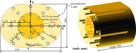
Design of an elliptical-shaped body phantom with tissue-equivalent material. Dose measurement inserts were placed at the 23 distributed points as shown in the axial view. Rods of equivalent material were placed in all holes that were not being used for dose measurement.
2.A.2. IC dose point measurements
The delivered dose within the phantom was measured using a single Nuclear Enterprise 2571 (0.6 cm3) Farmer-type small IC connected to a CNMC K602 Precision Electrometer sequentially at the 23 distributed points, following the AAPM TG111 approach.8 The IC was calibrated at an accredited dosimetry calibration laboratory over the beam quality ranges of our C-arm CT system. An f-factor [exposure-to-dose conversion factor, Gy/(C/kg)]22 of 0.876 was used. The presence of the IC was shown not to perturb the AEC response, including tube voltage and tube current-time product per projection.5 The IC measured the peak dose D(0) at the center of the z-extent of the body phantom.
The delivered dose within the phantom was measured for several different acquisition protocols including the two different minimum values of the kVp allowed (109 and 125 kVp), detector dose request of 0.36 μGy/projection, and three different sizes of z-collimator aperture at the isocenter: full: 22.2 cm (28.0 cm at the detector), medium: 14.0 cm (17.5 cm at the detector), and small: 8.4 cm (10.5 cm at the detector). Our C-arm CT system (Axiom Artis dTA, Siemens Medical Solutions, Forchheim, Germany) acquired 396 projection images/reconstruction (8-s scan) with a 0.5° angular step and used a large x-ray focal spot size (0.9 mm). Detailed acquisition parameters are provided in Table I. We acquired data for six different acquisition protocols:
TABLE I.
Acquisition parameters for IC dose point measurements and MC simulation. The values of the protocols were acquired from the C-arm CT system.
| Parameters | Values |
|---|---|
| Minimum value of the kVp allowed (kVp) | 109, 125 |
| Detector dose request (μGy/projection) | 0.36 |
| Number of projections | 396 |
| C-arm angular coverage (deg) | 200 |
| Size of z-collimator aperture at isocenter (cm) | Full: 22.2 |
| Medium: 14.0 | |
| Small: 8.4 | |
| Source to detector distance (mm) | 1198 |
| Source to patient distance (mm) | 785 |
| X-ray beam cone and fan angle (deg) | 6.7 and 9.0 |
| Half-value layer at 109 and 125 kV (mm Al) | 4.3 and 4.7 |
(i) Acquisition 1: 125 kVp, full collimation (22.2 cm),
(ii) acquisition 2: 125 kVp, medium collimation (14.0 cm),
(iii) acquisition 3: 125 kVp, small collimation (8.4 cm),
(iv) acquisition 4: 109 kVp, full collimation (22.2 cm),
(v) acquisition 5: 109 kVp, medium collimation (14.0 cm),
(vi) acquisition 6: 109 kVp, small collimation (8.4 cm).
2.A.3. Monte Carlo (MC) simulations
A MC simulation model was developed using geant4 (GEometry ANd Tracking)23 to generate 2D dose profiles over the central plane of the body phantom. The geant4 (version 9.4, patch 03) model used the standard electromagnetic physics list option 3, which is suitable for medical applications. The responses of the AEC (tube voltage and tube current-time product) for an individual projection were exported and used to characterize our C-arm CT system’s x-ray output. The x-ray spectra of the peak voltage (kVp) were generated in energy ranges of 10–150 keV with energy intervals of 1 keV, using the algorithm of Tucker et al.24 The output of the point x-ray spectra produced photon flux per tube current-time product in units of photon number/(mm2 mAs). The x-ray spectra were adjusted such that the half-value layer (HVL) of MC simulations corresponded with that of our C-arm CT system at the four tube voltages (70, 81, 109, and 125 kVp). The same geometric parameters (Table I) and the same body phantom geometry (Fig. 1) used in the experiment were implemented in the MC simulations via the DICOM image import feature of geant4. The CT numbers of air and the body phantom were converted to physical densities and element composition to provide voxelized material information.
The simulation model was validated at the 23 dose points against IC experimental data for the six different acquisition protocols. The simulation results correspond to a total of approximately 1 × 10⁶ incoming x-rays. The simulated photon fluences were 5 orders of magnitude below those of the experiment. The absolute dose calibration of the MC model was performed using the ratio of the 23 IC absolute doses to the MC (Gy per incident particle) dose points at the same positions, as in Downes et al.25
The mean dose () of the acquired 2D dose profiles in the central phantom plane for each acquisition protocol was used as a ground truth for the mean dose estimation methods introduced in Subsection 2.B.
2.B. Proposed mean dose methods for the body phantom
Conventional mean dose metrics, such as CTDIw, do not translate easily to C-arm CT body applications because the weighting factors in the conventional methods do not account for the highly asymmetric dose distribution from partial rotation over π + fan and nonuniform AEC response over the noncylindrical body phantom. Herein, we define two new methods, a proximity-based weighting method and a point surface fitting method, to calculate the mean dose for the body phantom.
2.B.1. Method 1: Proximity-based weighting method
The proximity-based weighting method defined here (hereafter, referred to as “method 1”) can be interpreted as a Riemann sum to approximate the area underneath the 2D dose profiles over the central phantom plane using a small number of regions. Method 1 computed the mean dose as shown in Fig. 2. First, the 23 dose points were grouped into two central regions (C1 and C2) and two peripheral regions (P1 and P2), as shown in Fig. 2(a). Second, the ratios of the areas associated with each of the dose points were calculated based on each voxel’s proximity to the points. As shown in (b), the voxels in the body phantom were clustered based on the distance from the voxels to their closest point, and thus, the body phantom was divided into 23 different clusters associated with each dose point. We assumed that the dose to the voxels in each cluster was best represented by the closest dose point. The weight (wi) of the ith dose point was defined as the area of its associated cluster over the total area of the central phantom plane. The sum of the acquired weights of the dose points in the same region was defined as the region’s weight (WC1,C2,P1,P2) as follows:
| (1) |
where i is the ID of dose points in each region. The resulting values of WC1, WC2, WP1, and WP2 were 0.0510, 0.3120, 0.3177, and 0.3193, respectively. Each region’s weight was proportional to the area of each region’s associated voxels, as shown in (c). Last, the mean IC reading of each of the four regions was summed after weighting by the acquired regional weights, as follows:
| (2) |
where is the estimated mean dose and indicates each region’s mean IC reading. Note that the regional weights did not change, while the regional mean IC readings depended on the number of dose points and their displacement, as described further in Subsection 2.B.4.
FIG. 2.
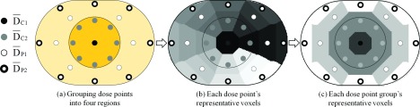
Steps for region-weighted sum method. For the proposed mean dose metrics, the 23 dose points were grouped into four regions (C1, C2, P1, and P2), as shown in (a). represents the average dose of the dose points in region C1 and (b) shows each dose point’s representative voxels based on each point’s closeness to the voxels. Then, the voxels of the dose points in the same region were grouped as shown in (c).
2.B.2. Method 2: Dose point surface fitting method
Although method 1 is simple to use, we can expect it to be somewhat inaccurate, as it uses only a small number (four) of regions for the Riemann sum of the 2D dose profile. Using individual voxels as a region to take an integral of the 2D dose profile helps mitigate inaccuracy, and thus, we surface-interpolated the dose profile over the central phantom plane. The dose point surface fitting method introduced here (hereafter, referred to as method 2) computed the mean dose as shown in Fig. 3. First, we chose the number of dose points to use and their distribution, as shown in (a). Given the trajectory of the C-arm gantry, the dose profiles are likely to be symmetric about the y-axis in (b), and thus, the dose points were mirrored on the other side of the axis of symmetry to distribute the dose points uniformly over the entire central plane of the body phantom. Then, as shown in (c), the surface interpolation model was used to interpolate the dose points, including the mirrored points. Last, the mean dose was computed as follows:
| (3) |
where x and y are the coordinates of the voxels in the central plane of the body phantom shown in Fig. 1, and F is the surface interpolant.
FIG. 3.
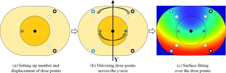
Steps for dose point surface fitting method. Six dose points from four regions were well distributed, as shown in (a). (b) shows the dose points and their mirrored dose points across the y-axis. Using the dose points, including the mirrored dose points as a control point, surface fitting over the body phantom was conducted, as shown in (c).
We selected the biharmonic spline interpolation model (see Appendix) from among various surface interpolants, as it functions especially well for generating smooth surfaces using irregularly spaced and sparse control points with noise.26 Moreover, it is available as option v4 in matlab (The MathWorks, Inc.).
2.B.3. Current CTDIw-like method
For purposes of comparison, we also computed the current CTDIw-like method, as follows:
| (4) |
where DC and are the central axis dose and the average of the peripheral axis doses, respectively, and WC and WP are the weighting factors for the central and peripheral axes, respectively.5 This method is identical to the conventional CTDIw, except that it uses the peak dose D(0) from IC measurements rather than from CTDI. The dose point measurement locations for this method are shown at the end of Fig. 4. For convenience, we labeled the resulting mean doses with WC = 1/3 and WP = 2/3 as “CTDIw(1/3, 2/3)”27 and with WC = 1/2 and WP = 1/2 as “CTDIw(1/2, 1/2).”15
FIG. 4.
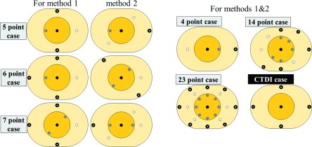
Tested dose point distributions. Six different cases of dose point numbers were tested, and some of the cases had different dose point distributions. The last distribution, “CTDI case,” shows the dose point measurement locations for CTDI.
2.B.4. Dose point distribution configurations
We tested different dose point distributions with different numbers of dose points to determine the minimum number of measurements needed to estimate the mean dose of a given acquisition protocol using the proposed methods. We constrained the number of possible distributions by making the following four assumptions:
-
(1)
The body phantom is assumed to be positioned at the isocenter of the C-arm CT system.
-
(2)
The first and second quadrants of the body phantom have a symmetrical dose distribution, and the third and fourth quadrants are also symmetric. Therefore, the dose points on the right side of the y-axis can represent the dose points on the other side of the axis, and vice versa.
-
(3)
The doses measured above and below the x-axis are not symmetric. Thus, if a dose point on either sides of the x-axis is chosen, the dose point located at the mirrored position should also be chosen.
-
(4)
Uniform dose point distribution is preferable to bunched points for incorporating more global dose profiles. (4-1) Thus, each region (C1, C2, P1, and P2) in Fig. 2(a) has to have at least one dose point measurement. (4-2) Moreover, unless only one dose point is available in a region, evenly distributed dose points on both sides of the y-axis are preferable to dose points grouped on either sides of the y-axis.
Thirty different dose point distributions in total resulted from the four assumptions described above. We tested six different cases of each dose point number (4, 5, 6, 7, 14, and 23), each of which had different dose point distributions. The performance of each distribution was measured in terms of relative difference (%), i.e., the differences between the mean dose estimated by either of the methods () with each distribution and the mean dose from MC simulations (), according to the following equation:
| (5) |
Among all of the possible dose point distributions, the best distributions for each point number case with the smallest difference [Eq. (5)] were shown in Fig. 4.
2.B.5. Performance of the methods in the presence of measurement uncertainties
An analysis of the sensitivity of the methods’ performances as a function of the level of measurement uncertainties helps to identify which error types contribute the most to performance degradation. We measured the dose of the two dose points ten times at three different positions (isocenter, 1 cm below and 3 cm below), as shown in Table II. The mean dose point readings were found to be sensitive to the displacement of the phantom from the isocenter. The mean readings of the two points changed 38.89% and −9.05%, respectively, in response to displacement as small as 1 cm from the y-axis. On the other hand, the two dose points’ random errors (σ, i.e., the standard deviation of the repeated measurements) were an average of 0.42%, corresponding to the repeatability of the IC measurements’ setup of 0.4% in Descamps et al.28 That is to say, systematic errors due to phantom displacement were much larger than those of the random error of IC readings, and thus, the random error was excluded from the error sensitivity analysis of the methods.
TABLE II.
The mean and random error (σ, mGy and %) of two dose points (see the diagrams below) at different phantom positions relative to the isocenter. The body phantom was shifted by 1 and 3 cm below the isocenter in the y-axis.

|

|
|||||
|---|---|---|---|---|---|---|
| Isocenter | 1 cm below | 3 cm below | Isocenter | 1 cm below | 3 cm below | |
| Mean, mGy | 26.92 | 37.39 | 48.94 | 113.31 | 103.06 | 90.52 |
| σ, mGy | 0.14 | 0.25 | 0.06 | 0.47 | 0.57 | 0.25 |
| σ, % | 0.50 | 0.67 | 0.13 | 0.41 | 0.55 | 0.28 |
In order to track the methods’ performances at different phantom locations from the isocenter, we shifted the body phantom by 1, 2, and 3 cm along either the x-axis or the y-axis using the x-ray outputs from Acquisition 1 and Acquisition 4. The difference metric used in this subsection was similar to Eq. (5), except that the absolute values were not taken in order to permit tracking of difference variations as a function of phantom displacement,
| (6) |
where and were the average of two representative acquisitions (acquisition 1 and acquisition 4) of 109 and 125 kV, respectively.
2.C. Generalization of the methods to a broad range of acquisition parameters
2.C.1. Usage of the methods in body phantoms of different dimensions
Radiation doses in patients are closely related to patients’ dimensions and the x-ray source output. Using a CTDIvol acquired from scanning a large phantom to estimate the dose for small patients could lead to considerably underestimating the dose level.26 Thus, body phantoms must be scaled to address size-specific doses. We applied the proposed methods to body phantoms of three different dimensions that represented the lower bounds and upper bounds of the adult population. Note that the body phantom dimension represents the average size of the adult population. We set the width of the lower bound body phantom to the 5th percentile interscye (324 mm) for the adult female.20 Then, we scaled the remaining dimensions (e.g., height) linearly, based on the ratio of the interscye dimension to the body phantom width. We set the width of the upper bound body phantom to the 95th percentile (454 mm) for the adult male20 and scaled other dimensions in a similar fashion. The resulting dimensions (width × height in mm) for the lower bound and upper bound body phantoms were determined as follows:
(i) Lower bound: 324 × 228 mm,
(ii) upper bound: 454 × 319 mm.
We used acquisition 1 (i.e., 125 kVp, full) for the MC simulation using the three scaled body phantoms.
2.C.2. Use of the methods in a Philips C-arm CT scanner
To evaluate the robustness of the proposed methods with different acquisition parameters, a second C-arm CT scanner from a major CT scanner vender was investigated: Philips Allura Xper FD20 Angiography Suite (Philips Medical Systems, Cleveland, OH). The delivered dose within the phantom was measured using an “Abdomen/Thorax Xper CT, 123 kVp” acquisition protocol with different sizes of z-collimator aperture at the isocenter: full, 20.0 cm; medium, 12.6 cm; and small, 6.24 cm. The system acquired 313 projection images/reconstruction with a 0.67° angular step. The minimum allowed value of the kVp was 123 kVp with a HVL of 5.4 mm Al. After incorporating geometry, spectra, and AEC modulation of the tube voltage and the tube current-time product of the Philips FD20 system, the same MC simulation model described above was used to generate 2D dose profiles in the central phantom plane.
3. RESULTS
3.A. Measured IC dose point
Table III shows the measured delivered dose within the body phantom using a small IC at the 23 distributed points for acquisitions 1–6. As a narrower z-collimator aperture was used, the mean of the IC readings decreased at both the 109-kVp and the 125-kVp acquisitions. The mean of the IC readings at the 109-kVp protocols was higher than that at the 125-kVp protocols with the same size of the z-collimator aperture (e.g., acquisition 1 vs acquisition 4). Table IV shows that the MC simulation model was validated at the 23 dose points against IC experimental data (Table III) for the six different acquisition protocols with differences below 2 mGy/IC (1.69 mGy [±0.77 mGy]) and the Pearson product-moment correlation coefficient (Pearson’s r)29 of 0.965.
TABLE III.
The measured dose (mGy) within the body phantom using a small IC at the 23 distributed points. The mean, minimum, and maximum values of the IC reading for each acquisition protocol were reported. Note that detector dose request of 0.36 μGy/projection was used and “coll.” = the z-collimator aperture size.
| 125 kVp (minimum kVp allowed) | 109 kVp (minimum kVp allowed) | |||||
|---|---|---|---|---|---|---|
| (mGy) | Acquisition 1, full coll. | Acquisition 2, medium coll. | Acquisition 3, small coll. | Acquisition 4, full coll. | Acquisition 5, medium coll. | Acquisition 6, small coll. |
| Mean | 50.7 | 48.7 | 43.9 | 52.6 | 50.1 | 45.0 |
| Min | 9.0 | 7.6 | 6.0 | 8.7 | 7.6 | 5.9 |
| Max | 104.0 | 107.1 | 103.3 | 103.4 | 108.7 | 108.0 |
TABLE IV.
The validation of the MC simulation model against the 23 measured dose points (mGy) within the body phantom. The error values (i.e., the differences between the model and the IC reading) and Pearson’s r for six acquisition protocols (acquisition 1–6) were reported.
| 125 kVp (minimum kVp allowed) | 109 kVp (minimum kVp allowed) | ||||||
|---|---|---|---|---|---|---|---|
| Acquisition 1 | Acquisition 2 | Acquisition 3 | Acquisition 4 | Acquisition 5 | Acquisition 6 | Total (±σ) | |
| Error, mGy | 0.98 | 1.04 | 0.96 | 2.37 | 2.47 | 2.35 | 1.69 (±0.77) |
| Pearson’s r | 0.989 | 0.989 | 0.991 | 0.944 | 0.942 | 0.944 | 0.965 |
3.B. MC simulations
3.B.1. X-ray source output from the C-arm CT system
Figure 5 shows that the AEC of our Siemens system modulated the product of the tube current and exposure time (mAs), and the tube voltage as a function of the spatial gantry angle in response to the six different protocol requests (acquisitions 1–6). In general, the AEC increased the tube settings (tube voltage and tube current-time product) for projections with large x-ray attenuation (i.e., lateral views corresponding to the projection numbers around the first and last projections) and decreased the settings for projections with small attenuation [i.e., anteroposterior (AP) views corresponding to the projection numbers around the middle projection]. Thus, the variations in tube voltage and tube current-time product along the projection number were close to a symmetric distribution about the central projection number. For the 109-kVp protocols (acquisitions 4–6), the AEC increased tube current-time product first as the gantry rotated from the AP views to the lateral views, and then the AEC started to increase tube voltage to allow higher photon penetration and a greater number of photons after the tube reached its mAs maximum. At 125-kVp protocols (acquisitions 1–3), the values of tube voltage stayed constant while mAs was modulated similar to mAs at 109-kVp protocols, except that at 125-kVp protocols, mAs stayed at values below those at the first projection (reference mAs), because the high tube voltage (125 kV) was sufficient to maintain image quality. Although the AEC response of the Philips FD20 system for the 123-kVp protocol is not reported here, the system showed a mAs-dominant modulation with a minor change in the tube voltage (120–123 kV), which is similar to the modulation of the Siemens system for 125-kVp protocols (acquisitions 1–3).
FIG. 5.
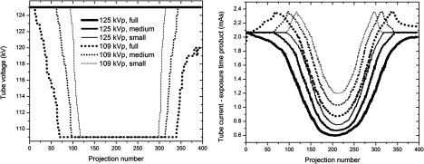
Built-in AEC system responses to the requested dose settings (acquisitions 1–6). The labels, e.g., “109 kVp, full,” refer to (1) a minimum value of the kVp allowed and (2) the size of the collimator used for the scan.
3.B.2. 2D dose profiles at the central phantom plane
Figure 6 shows the 2D dose distribution in the central plane (z = 0, i.e., the maximum dose image) of the body phantom; Figures (a1)–(b3) correspond to acquisitions 1–6, respectively. In general, the dose distributions had a C shape along the trajectory of the x-ray source from its starting point (shown in Fig. 1) after a 200° clockwise rotation. When a narrower z-collimator aperture was used, the computed mean dose decreased at both the 125-kVp and the 109-kVp acquisition protocols, and the dose distribution showed less radial variation due to reduced scatter, with a thinner C shaped higher dose region. The computed mean doses from the distributions at 125 kVp, acquisitions 1–3, were 51.25, 49.41, and 43.67 mGy, respectively. The mean doses of the dose distributions at 109 kVp, acquisitions 4–6, were 55.27, 51.46, and 46.20 mGy, respectively. The AEC modulation along the projection number showed nearly symmetric distribution about the central projection number, as shown in Fig. 5. Likewise, the central plane image had an almost symmetrical dose distribution about the vertical axis (y-axis) of the body phantom.
FIG. 6.
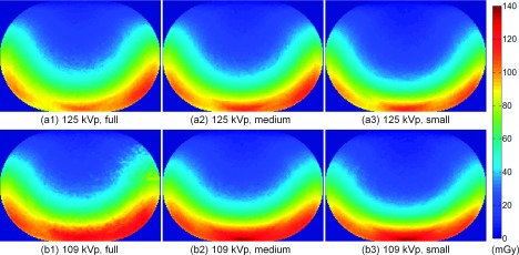
Dose distributions delivered to the central plane of the body phantom. The delivered dose was simulated for acquisitions 1–6, shown in [(a1)–(b3)].
3.C. Performance of the proposed methods
The metrics of the two proposed methods were computed using Eq. (5), and then the performances were compared for the different measurement point distributions, as summarized in Table V. To compare the performances of the two methods visually, we plotted their computed performance as a function of the number of dose points used (Fig. 7). Except for the 4-dose point case, the rest (5, 6, 7, 14, and 23) had differences below 3%, ranging from 0.5% to 2.9%. The two methods with the 5-, 6-, and 7-point cases showed performances comparable to those with a relatively large number of dose points, i.e., the 14 and 23 dose point cases. For 7 or fewer dose measurement points, the 7-point case (1.0% difference) and the 6-point case (0.7% difference) performed the best for method 1 and method 2, respectively. Using as few as five dose points, method 1 and method 2 achieved 1.7% and 1.3% differences, respectively. Both methods showed a sudden decrease in performance with the 4-point case, displaying relatively large differences and standard deviations when compared to the other dose point cases (see Fig. 7).
TABLE V.
Comparisons of the performances of the proposed methods using six different cases of each dose point number. Relative differences (%) of the methods were computed based on the differences between their values and those of the MC simulations. The reported values are the mean and the relative standard deviation (σ) of the performances of acquisitions 1–6.
| Method 1 | Method 2 | |
|---|---|---|
| Dose point number | Difference (±σ), % | Difference (±σ), % |
| 4 | 5.6 (±4.9) | 8.4 (±4.2) |
| 5 | 1.7 (±1.2) | 1.3 (±1.0) |
| 6 | 1.1 (±1.1) | 0.7 (±0.6) |
| 7 | 1.0 (±0.6) | 1.3 (±0.8) |
| 14 | 2.9 (±1.1) | 1.0 (±0.8) |
| 23 | 2.2 (±0.5) | 0.5 (±0.4) |
FIG. 7.

Comparison of the performances of the proposed methods as a function of the number of dose points used (4, 5, 6, 7, 14, and 23). The differences of CTDIw(1/3, 2/3) and CTDIw(1/2, 1/2) were 8.7% (±2.8%) and 6.8% (±1.0%), respectively.
Line profiles were drawn along the horizontal and vertical directions of the body phantom, resulting from the two methods in combination with each dose point case (4, 5, 6, 7, 14, and 23), as shown in Fig. 8. As expected, method 1, shown in (a1)–(a3), generated stair-like line profiles. The four stairs from the center to the outside in the horizontal profile in (a2) correspond to the four regions (C1, C2, P1, and P2, respectively) shown in Fig. 2(c). The width of the stairs was determined by each region’s weight as defined by Eq. (1). While the widths of the stairs did not change, regardless of the different distributions, the depths of the stairs varied depending on the values of the dose points belonging to each of the regions. Except for the line profiles of the 4-point case (distribution 4-1), those of the other dose point cases nearly overlapped. For method 2, the line profiles of all of the dose point cases almost overlapped in the horizontal direction [Fig. 8(b2)] and were close to each other, except for the 4-point case in the vertical direction [Fig. 8(b3)]. The line profiles of method 2 propagated smoothly through the control points (i.e., dose points). Because of the absence of a control point in the 4-point case in the vertical direction, the line profile deviated more from the MC simulation than did the other dose point cases. Moreover, method 2 demonstrated high-fidelity surface reconstruction with the 5-, 6-, and 7-point cases with their best distribution, showing pixelwise absolute differences of 3.8 mGy (±0.3 mGy), 4.0 mGy (±0.4 mGy), and 3.5 mGy (±0.2 mGy), respectively, from the MC simulations for acquisitions 1–6.
FIG. 8.
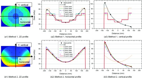
Horizontal and vertical line profiles of the two methods extracted along the x-axis and the y-axis of the 2D dose distribution, respectively. “MC” is the Monte Carlo simulation, and “dose points” show the location of the control points for method 1 and method 2.
3.D. An analysis of performance sensitivity to measurement uncertainties
We tracked the performances of the two methods as a function of the phantom displacement from the isocenter in the horizontal direction (the x-axis), as shown in Fig. 9. We evaluate change in point measurements relative to the values at zero displacement. Because our main concern was the degree to which performance is expected to change in response to the level of the phantom displacement, in this subsection, we dealt with the difference deviations at different phantom locations. In general, the relative differences deviated in either the positive or the negative direction in proportion to the level of the phantom displacement, up to 3 cm. The 5-point case was more sensitive to the phantom displacement in the x- and y-axes than were the 6- and 7-point cases. The results for the vertical displacement were not reported in the figure. However, regardless of the choice of the method and the dose point case, the difference deviations from the rest of the distributions generally remained under about 2% up to the 2-cm displacement in the horizontal (x-axis) and the vertical (y-axis) directions.
FIG. 9.

Analysis of the sensitivity of the performances of the methods as a function of the phantom displacement from the isocenter. The performances of the methods were computed using the difference metric in Eq. (6) after shifting the body phantom by 1, 2, and 3 cm along the x-axis.
3.E. Performances of the methods with a broad range of acquisition parameters
Table VI shows the performances of the proposed methods as applied to body phantoms of different dimensions that represent the lower bound and upper bound of the adult population. Except for the difference resulting from method 1 with the 4-point case, the differences remained below 4%, regardless of the phantom dimensions and methods employed.
TABLE VI.
Application of the proposed methods to body phantoms of different dimensions scaled to the lower bound, mean bound, and upper bound. The performances of the methods were compared using different dimensions and six different cases of each dose point number. The dimensions (width × height in mm) of the lower bound and upper bound were 324 × 228 and 454 × 319, respectively. Relative differences (%) of the methods were computed based on their values’ absolute differences from MC simulations using Eq. (4).
| Difference of method 1, % | Difference of method 2, % | |||
|---|---|---|---|---|
| Used IC number | Lower bound | Upper bound | Lower bound | Upper bound |
| 5 | 3.4 | 4.0 | 2.1 | 0.2 |
| 6 | 0.5 | 1.1 | 3.2 | 2.9 |
| 7 | 0.5 | 0.9 | 0.2 | 1.6 |
Table VII shows the performances of the methods using the body acquisition protocol of the Philips FD 20 system with three different sizes for the z-collimator aperture. Again, except for the difference resulting from method 1 with the 5-point case, methods using 5-, 6-, and 7-point cases generally work well and produce differences of around 1%.
TABLE VII.
Comparisons of the performances of the proposed methods using 5-, 6-, and 7-point cases. Relative differences (%) of the methods were computed based on the differences between their values and those of the MC simulations. The reported values are the mean and the relative standard deviation (σ) of the performances of the Philips scanner acquisitions with three different sizes of z-collimator aperture.
| Dose point number | Method 1 difference (±σ), % | Method 2 Difference (±σ), % |
|---|---|---|
| 5 | 6.3 (±0.6) | 0.9 (±0.5) |
| 6 | 1.0 (±0.9) | 2.2 (±0.4) |
| 7 | 0.4 (±0.2) | 0.8 (±0.4) |
4. DISCUSSION
The two mean dose estimation methods introduced herein, which incorporate either proximity-based weighting (method 1) or 2D dose surface fitting (method 2), demonstrated reasonable accuracy in computing the mean dose at the central plane of the elliptical body phantom under the influence of the AEC modulation for acquisitions 1–6. For the purpose of minimizing the number of measurements required to characterize the dose distribution of a given acquisition protocol with reasonable accuracy, the 5-, 6-, and 7-point cases are preferable to the 14- and 23-point cases. While all of the 5-, 6-, and 7-point cases had differences below 2%, our results indicate that the 7- and 6-point cases are recommended for method 1 and method 2, respectively. Moreover, method 2 with the 5-, 6-, and 7-point cases demonstrated high-fidelity surface reconstruction, and thus we can use the reconstructed 2D dose profiles to estimate the internal organ dose and the peripheral skin dose after registering the respective body parts to the elliptical body phantom.
Method 1 and method 2 with as few as five dose points showed better performance in estimating the mean dose, with 1.7% (±1.2%) and 1.3% (±1.0%) differences, than the current CTDIw-like method, i.e., CTDIw(1/3, 2/3) and CTDIw(1/2, 1/2) with 8.7% (±2.8%) and 6.8% (±1.0%) differences. Between the two different weighting factors, CTDIw(1/2, 1/2) provided more accurate dose estimation than the conventional CTDIw(1/3, 2/3), which is consistent with Kim et al.,30 although they did not use exactly the same experimental setups as those in this study; they measured dose over a cylindrical body phantom without AEC modulation.
The performance of method 1 showed strong dependency on dose point distributions. The dose points in the outer peripheral region (i.e., region P2; see Fig. 2 for four regions in the phantom) especially affected method 1’s performance directly, because that region contains the highest and the lowest dose distribution; radiation dose drops off by the inverse square law and dose attenuation through the body phantom, resulting in the C-shaped dose distribution shown in Fig. 6. Moreover, region P2 has the highest regional weight (WP2) in Eq. (2) for method 1. The dose point distributions of the 5-, 6-, and 7-point cases with method 1 have region P2 dose points on the y-axis in common. The distributions with region P2 dose points on the diagonal line performed poorly with method 1, which means that the mean of the diagonal dose points does not accurately represent the mean dose of region P2. Despite having more dose points, the 14- and 23-point cases did not show better performance than the 5-, 6-, and 7-point cases. However, after taking out the region P2 diagonal dose points from the 14 dose point case, the performance sharply improved from 2.9% (±1.1%) difference to 0.8% (±0.3%) difference. These observations indicate that more dose points do not guarantee better performance of a weighting-based mean dose estimation method and that a choice of dose point placement is significant for better performance. Another concern for the dose points in region P2 is that they are placed close to the outer edge of the P2 region’s stair rather than at the center of the stair, as shown in Figs. 8(a2) and 8(a3). Considering that the dose falls off quickly when approaching the phantom surface, the dose point weighted toward the outer edge of the P2 stair overestimates the dose to the front side of the phantom and underestimates the dose to the back of the phantom. Further improvement of method 1 can be made by implementing a different weighted sum scheme (e.g., the trapezoidal sum), which could compensate for the onside dose point.
Similar to method 1, method 2’s performance also strongly depended on dose point distributions, especially the dose points in the peripheral region of the body phantom. However, in contrast to method 1, method 2 performed well with the distributions with peripheral dose points on the diagonal line rather than with peripheral dose points on the y-axis. This finding is also confirmed by the fact that after removing the region P2 diagonal dose points from the 14-point case, the performance rapidly decreased from 1.0% (±0.8%) difference to 4.5% (±1.1%) difference. This result might be due to the elliptical shape of the body phantom, as the dose profile along the diagonal line is much longer than that along the vertical line. Thus, missing the control points at both ends of the diagonal line has a broader impact on the reconstructed surface fidelity than losing the points on the vertical line. The biharmonic interpolant used for method 2 is very smooth compared to alternative interpolation methods, including polynomial interpolation, neighborhood-based methods, and harmonic interpolation.31 The smoothness comes about because each dose point’s force is determined in relation to radial basis functions defined for all other points, as shown in Appendix. Nonsmooth interpolants are not well suited for this application, where control points are sparse, given the size of the body phantom, since the interpolations respond to noisy dose point measurements with sudden bumps and overshoot characteristics which we do not see in our 2D dose profile.
The analysis of the methods’ sensitivity to measurement uncertainties (Subsection 3.D) showed that performance was highly sensitive to the alignment of the body phantom relative to the image acquisition system. If a dose point comes closer to the x-ray source due to the phantom shift, the dose point will receive higher exposure due to the inverse square law, and the dose points on the opposite quadrant of the phantom will receive less exposure as they move away from the x-ray source, as shown in Table II. Accordingly, the C-shaped dose distribution will change in intensity and shape, and therefore, the second assumption (Subsection 2.B.4) of a symmetrical dose distribution about the y-axis may become inaccurate. In order to prevent geometrical differences of more than about 2%, care needs to be taken to align the system precisely within 2 cm on both the x- and y-axes. The analysis also implies that when we make a choice of dose point distributions, we should consider the methods’ robustness to the phantom misalignment.
Method 1 and method 2 performed well with the two differently scaled body phantoms, representing the lower bound and upper bound of the adult population. Evaluating the two methods with the different phantoms is valuable in that the radiation dose for a patient is closely correlated with the size of the patient.26 Therefore, the mean dose cannot represent a patient dose if the phantom size is significantly different from the patient’s size. Recently, AAPM Report 204 (Ref. 32) and 220 (Ref. 33) introduced approaches for size-specific dose estimation (SSDE). They provide a conversion factor that translates CTDIvol into a patient-specific dose that is based on geometric patient size32 and patient attenuation,33 respectively. Compared to the geometric-based metric, the attenuation based-metric is less practical due to its complexity but provides more accurate dose estimates especially for the thoracic (lung) region.33
As shown in Subsection 3.B.2, narrow collimation imaging decreases the mean dose in the plane of maximum dose (z = 0) because it decreases total volume irradiated, and thus, reduces scattering impact on the central dose. Moreover, narrow collimator imaging increases detectability, because scattering then has less of an effect on image quality in body imaging. It has been shown that a small FOV (i.e., acquisition 3) has a 9% higher detectability than a large FOV (i.e., acquisition 1) for the 125-kVp acquisition.34 Although the tube voltage difference had a relatively minor impact on the estimated mean dose, smaller objects were more detectable with the minimum 109-kVp request than with the minimum 125-kVp request.34 Therefore, in addition to narrow collimation imaging, a minimum tube voltage request of 109 kVp is recommended for C-arm CT body applications.
The proposed methods were evaluated for various acquisition parameters including different kVp requests and different z-collimator aperture sizes for the C-arm CT scanners from two major venders. As long as the CT system modulates the x-ray photon fluence smoothly frame by frame during scanning, the methods are expected to perform well for the resulting smooth dose surface. It is of interest to include evaluations of the methods over a broader range of CT operating conditions that affect the dose profiles, such as different AEC systems35 and bow-tie filters.36 However, different AEC techniques and bowtie filters would only have most probably minor impacts on the performances of the proposed methods because AEC modulates the x-ray photons based on the slowly varying penetration depth of the body phantom and the bowtie filter attenuation profile is designed to incorporate a cylinder-like human body.
5. CONCLUSIONS
We introduced two dose point-based methods, the proximity-based weighting (method 1) and the 2D dose surface fitting (method 2) to characterize the mean dose, , and the 2D dose distribution, D (x,y), in the central peak-dose image (z = 0) of the elliptical body phantom from AEC-enabled partial C-arm CT scans without table translation. With as few as five dose points, both methods computed the mean dose with reasonable accuracy, demonstrating 1.7% (±1.2%) and 1.3% (±1.0%) differences, respectively. A larger number of dose points does not necessarily guarantee better performance of the methods (especially method 1), and an optimal choice of dose point placement is significant for better performance. Because the performance of the methods is sensitive to the alignment of the center of the body phantom relative to the isocenter, careful alignment within 2 cm in both the x- and y-axes is required to ensure less than 2% geometrical differences. Among the 5-, 6-, and 7-point cases, the 7- and the 6-point cases are recommended for method 1 and method 2, respectively, demonstrating a minimum difference of less than 1%. Although method 2 is more computationally demanding than method 1, in applications where dose distributions are important, method 2 should be used because it reconstructs the dose surface using as few as five dose points with high fidelity with differences of only 3.8 mGy (±0.3 mGy).
ACKNOWLEDGMENTS
This work was supported in part by NIH 1 R01HL087917, NIH Shared Instrument Grant No. S10 RR026714 supporting the zeego@StanfordLab, and Siemens AX.
APPENDIX: BIHARMONIC SPLINE INTERPOLATION IN 2D
In this study, we want to determine a biharmonic function passing through N number of the IC control points in 2D. The fitting spline uses the Green’s function for a point force to interpolate the reading values of the IC points (zi) positioned at xi. The problem in 2D becomes
| (A1) |
| (A2) |
where αj is the strength of each IC point force which can be computed by solving the linear system of either slopes or values of the IC reading and ∇4 is the biharmonic operator. The general solution to Eqs. (A1) and (A2) is
| (A3) |
where Green function and its gradient . The detailed derivation of the solution can be found in the work of Sandwell.37
REFERENCES
- 1.Orth R. C., Wallace M. J., and Kuo M. D., “C-arm cone-beam CT: General principles and technical considerations for use in interventional radiology,” J. Vasc. Interv. Radiol. 19(6), 814–820 (2008). 10.1016/j.jvir.2008.02.002 [DOI] [PubMed] [Google Scholar]
- 2.Wallace M. J., Kuo M. D., Glaiberman C., Binkert C. A., Orth R. C., Soulez G., and Soc T. A. C., “Three-dimensional C-arm cone-beam CT: Applications in the interventional suite,” J. Vasc. Interv. Radiol. 19(6), 799–813 (2008). 10.1016/j.jvir.2008.02.018 [DOI] [PubMed] [Google Scholar]
- 3.Siewerdsen J. H., Moseley D. J., Burch S., Bisland S. K., Bogaards A., Wilson B. C., and Jaffray D. A., “Volume CT with a flat-panel detector on a mobile, isocentric C-arm: Pre-clinical investigation in guidance of minimally invasive surgery,” Med. Phys. 32(1), 241–254 (2005). 10.1118/1.1836331 [DOI] [PubMed] [Google Scholar]
- 4.Choi J.-H., Maier A., Keil A., Pal S., McWalter E. J., Beaupré G. S., Gold G. E., and Fahrig R., “Fiducial marker-based correction for involuntary motion in weight-bearing C-arm CT scanning of knees. II. Experiment,” Med. Phys. 41, 061902(16pp.) (2014). 10.1118/1.4873675 [DOI] [PMC free article] [PubMed] [Google Scholar]
- 5.Fahrig R., Dixon R., Payne T., Morin R. L., Ganguly A., and Strobel N., “Dose and image quality for a cone-beam C-arm CT system,” Med. Phys. 33(12), 4541–4550 (2006). 10.1118/1.2370508 [DOI] [PubMed] [Google Scholar]
- 6.Jucius R. A. and Kambic G. X., “Radiation dosimetry in computed tomography (CT),” Proc. SPIE 0127, Application of Optical Instrumentation in Medicine VI (1977), pp. 286–295. 10.1117/12.955952 [DOI] [Google Scholar]
- 7.Shope T. B., Gagne R. M., and Johnson G. C., “A method for describing the doses delivered by transmission-x-ray computed-tomography,” Med. Phys. 8(4), 488–495 (1981). 10.1118/1.594995 [DOI] [PubMed] [Google Scholar]
- 8.Dixon R., Anderson J., Bakalyar D., Boedeker K., Boone J., Cody D., Fahrig R., Jaffray D., Kyprianou I., and McCollough C., “Comprehensive methodology for the evaluation of radiation dose in x-ray computed tomography,” Report No. 111, Report of AAPM Task Group 111 (American Association of Physicists in Medicine, 2010). [Google Scholar]
- 9.Dixon R. L. and Boone J. M., “Cone beam CT dosimetry: A unified and self-consistent approach including all scan modalities-with or without phantom motion,” Med. Phys. 37(6), 2703–2718 (2010). 10.1118/1.3395578 [DOI] [PMC free article] [PubMed] [Google Scholar]
- 10.Dixon R. L. and Boone J. M., “Stationary table CT dosimetry and anomalous scanner-reported values of CTDIvol,” Med. Phys. 41(1), 011907(6pp.) (2014). 10.1118/1.4845075 [DOI] [PubMed] [Google Scholar]
- 11.Dixon R. L., “A new look at CT dose measurement: Beyond CTDI,” Med. Phys. 30(6), 1272–1280 (2003). 10.1118/1.1576952 [DOI] [PubMed] [Google Scholar]
- 12.Turner A. C., Zankl M., DeMarco J. J., Cagnon C. H., Zhang D., Angel E., Cody D. D., Stevens D. M., McCollough C. H., and McNitt-Gray M. F., “The feasibility of a scanner-independent technique to estimate organ dose from MDCT scans: Using CTDIvol to account for differences between scanners,” Med. Phys. 37(4), 1816–1825 (2010). 10.1118/1.3368596 [DOI] [PMC free article] [PubMed] [Google Scholar]
- 13.Turner A. C., Zhang D., Khatonabadi M., Zankl M., DeMarco J. J., Cagnon C. H., Cody D. D., Stevens D. M., McCollough C. H., and McNitt-Gray M. F., “The feasibility of patient size-corrected, scanner-independent organ dose estimates for abdominal CT exams,” Med. Phys. 38(2), 820–829 (2011). 10.1118/1.3533897 [DOI] [PMC free article] [PubMed] [Google Scholar]
- 14.Khatonabadi M., Kim H. J., Lu P., McMillan K. L., Cagnon C. H., DeMarco J. J., and McNitt-Gray M. F., “The feasibility of a regional CTDIvol to estimate organ dose from tube current modulated CT exams,” Med. Phys. 40(5), 051903(11pp.) (2013). 10.1118/1.4798561 [DOI] [PMC free article] [PubMed] [Google Scholar]
- 15.Bakalyar D. M., “A critical look at the numerical coefficients in CTDIVOL,” Med. Phys. 33(6), 2003 (2006). 10.1118/1.2240267 [DOI] [Google Scholar]
- 16.Feng W., Schultz C., Chen H., Chu A., Hu A., and Bakalyar D., “TU-FF-A4-04: Experimental confirmation of near parabolic shape of dose profile in cylindrical phantom for dual source CT,” Med. Phys. 34(6), 2571–2572 (2007). 10.1118/1.2761440 [DOI] [Google Scholar]
- 17.Fisher R. F., “Tissue equivalent phantoms for evaluating in-plane tube current modulated CT dose and image quality,” M.S. dissertation, University of Florida, 2006. [Google Scholar]
- 18.Sookpeng S., Martin C. J., and Gentle D. J., “A study of CT dose distribution in an elliptical phantom and the influence of automatic tube current modulation in the x-y plane,” J. Radiol. Prot. 33(2), 461–483 (2013). 10.1088/0952-4746/33/2/461 [DOI] [PubMed] [Google Scholar]
- 19.Sookpeng S., Martin C. J., and Gentle D. J., “Comparison of different phantom designs for CT scanner automatic tube current modulation system tests,” J. Radiol. Prot. 33(4), 735–761 (2013). 10.1088/0952-4746/33/4/735 [DOI] [PubMed] [Google Scholar]
- 20.Nasa, Man-Systems Integration Standards (NASA-STD-3001), Volume I, Section 3, Anthropometry and Biomechanics (1995).
- 21.Dixon R. L. and Ballard A. C., “Experimental validation of a versatile system of CT dosimetry using a conventional ion chamber: Beyond CTDI100,” Med. Phys. 34(8), 3399–3413 (2007). 10.1118/1.2757084 [DOI] [PubMed] [Google Scholar]
- 22.McCollough C., Cody D., Edyvean S., Geise R., Gould B., Keat N., Huda W., Judy P., Kalender W., and McNitt-Gray M., “The measurement, reporting, and management of radiation dose in CT,” Report of AAPM Task Group 23 (American Association of Physicists in Medicine, 2008). [Google Scholar]
- 23.Allison J., Amako K., Apostolakis J., Araujo H., Dubois P. A., Asai M., Barrand G., Capra R., Chauvie S., Chytracek R., Cirrone G. A. P., Cooperman G., Cosmo G., Cuttone G., Daquino G. G., Donszelmann M., Dressel M., Folger G., Foppiano F., Generowicz J., Grichine V., Guatelli S., Gumplinger P., Heikkinen A., Hrivnacova I., Howard A., Incerti S., Ivanchenko V., Johnson T., Jones F., Koi T., Kokoulin R., Kossov M., Kurashige H., Lara V., Larsson S., Lei F., Link O., Longo F., Maire M., Mantero A., Mascialino B., McLaren I., Lorenzo P. M., Minamimoto K., Murakami K., Nieminen P., Pandola L., Parlati S., Peralta L., Perl J., Pfeiffer A., Pia M. G., Ribon A., Rodrigues P., Russo G., Sadilov S., Santin G., Sasaki T., Smith D., Starkov N., Tanaka S., Tcherniaev E., Tome B., Trindade A., Truscott P., Urban L., Verderi M., Walkden A., Wellisch J. P., Williams D. C., Wright D., and Yoshida H., “Geant4 developments and applications,” IEEE Trans. Nucl. Sci. 53(1), 270–278 (2006). 10.1109/TNS.2006.869826 [DOI] [Google Scholar]
- 24.Tucker D. M., Barnes G. T., and Chakraborty D. P., “Semiempirical model for generating tungsten target x-ray-spectra,” Med. Phys. 18(2), 211–218 (1991). 10.1118/1.596709 [DOI] [PubMed] [Google Scholar]
- 25.Downes P., Jarvis R., Radu E., Kawrakow I., and Spezi E., “Monte Carlo simulation and patient dosimetry for a kilovoltage cone-beam CT unit,” Med. Phys. 36(9), 4156–4167 (2009). 10.1118/1.3196182 [DOI] [PubMed] [Google Scholar]
- 26.McCollough C. H., Leng S. A., Yu L. F., Cody D. D., Boone J. M., and Mcnitt-Gray M. F., “CT dose index and patient dose: They are not the same thing,” Radiology 259(2), 311–316 (2011). 10.1148/radiol.11101800 [DOI] [PMC free article] [PubMed] [Google Scholar]
- 27.Leitz W., Axelsson B., and Szendro G., “Computed-tomography dose assessment–A practical approach,” Radiat. Prot. Dosim. 57(1-4), 377–380 (1995). [Google Scholar]
- 28.Descamps C., Gonzalez M., Garrigo E., Germanier A., and Venencia D., “Measurements of the dose delivered during CT exams using AAPM Task Group Report No. 111,” J. Appl. Clin. Med. Phys. 13(6), 293–302 (2012). [DOI] [PMC free article] [PubMed] [Google Scholar]
- 29.Pearson K., “Note on regression and inheritance in the case of two parents,” Proc. R. Soc. London 58, 240–242 (1895). 10.1098/rspl.1895.0041 [DOI] [Google Scholar]
- 30.Kim S., Yoo S., Yin F. F., Samei E., and Yoshizumi T., “Kilovoltage cone-beam CT: Comparative dose and image quality evaluations in partial and full-angle scan protocols,” Med. Phys. 37(7), 3648–3659 (2010). 10.1118/1.3438478 [DOI] [PubMed] [Google Scholar]
- 31.Hale D., “Image-guided blended neighbor interpolation of scattered data,” in SEG Annual Meeting (Society of Exploration Geophysicists, Houston, TX, 2009). [Google Scholar]
- 32.Boone J., Strauss K., Cody D., McCollough C., McNitt-Gray M., Toth T., Goske M., and Frush D., “Size-specific dose estimates (SSDE) in pediatric and adult body CT examinations,” Report No. 204 (American Institute of Physics for the American Association of Physicists in Medicine, 2011). [Google Scholar]
- 33.McCollough C., Bakalyar D. M., Bostani M., Brady S., Boedeker K., Boone J. M., Chen-Mayer H. H., Christianson O. I., Leng S., Li B., McNitt-Gray M. F., Nilsen R. A., Supanich M. P., and Wang J., “Use of water equivalent diameter for calculating patient size and size-specific dose estimates (SSDE) in CT,” Report No. 220 (American Institute of Physics for the American Association of Physicists in Medicine, 2014). [PMC free article] [PubMed] [Google Scholar]
- 34.Choi J.-H., Constantin D., Nelson G., Ganguly A., Girard E., Morin R., Dixon R., and Fahrig R., “SU-D-103-02: Image quality assurance study of a cone-beam c-arm CT with automatic exposure control for body applications,” Med. Phys. 40(6), 110 (2013). 10.1118/1.4814040 [DOI] [Google Scholar]
- 35.Soderberg M. and Gunnarsson M., “Automatic exposure control in computed tomography–An evaluation of systems from different manufacturers,” Acta Radiol. 51(6), 625–634 (2010). 10.3109/02841851003698206 [DOI] [PubMed] [Google Scholar]
- 36.Nakonechny K. D., Fallone B. G., and Rathee S., “Novel methods of measuring single scan dose profiles and cumulative dose in CT,” Med. Phys. 32(1), 98–109 (2005). 10.1118/1.1835571 [DOI] [PubMed] [Google Scholar]
- 37.Sandwell D. T., “Biharmonic spline interpolation of Geos-3 and Seasat altimeter data,” Geophys. Res. Lett. 14(2), 139–142 (1987). 10.1029/GL014i002p00139 [DOI] [Google Scholar]