Isogeometric Kirchhoff-Love shell formulations for biological membranes

Abstract

Computational modeling of thin biological membranes can aid the design of better medical devices. Remarkable biological membranes include skin, alveoli, blood vessels, and heart valves. Isogeometric analysis is ideally suited for biological membranes since it inherently satisfies the C¹-requirement for Kirchhoff-Love kinematics. Yet, current isogeometric shell formulations are mainly focused on linear isotropic materials, while biological tissues are characterized by a nonlinear anisotropic stress-strain response. Here we present a thin shell formulation for thin biological membranes. We derive the equilibrium equations using curvilinear convective coordinates on NURBS tensor product surface patches. We linearize the weak form of the generic linear momentum balance without a particular choice of a constitutive law. We then incorporate the constitutive equations that have been designed specifically for collagenous tissues. We explore three common anisotropic material models: Mooney-Rivlin, May Newmann-Yin, and Gasser-Ogden-Holzapfel. Our work will allow scientists in biomechanics and mechanobiology to adopt the constitutive equations that have been developed for solid three-dimensional soft tissues within the framework of isogeometric thin shell analysis.

1. Motivation

Biological membranes appear often in nature, fulfilling crucial physiological roles for the survival of different forms of life. Perhaps one of the most evident examples is our skin, an essential barrier from the outside world with notable elastic properties [52]. Several other examples of membranes - although hidden to our eyes - are equally important because of their prominent functions: the alveoli, the pericardium, or the valve leaflets, to name just a few [41]. Characterizing the be-havior of these thin structures in distinct mechanical scenarios is key to improve our understanding of the mechanical aspects of disease and to design more effective medical devices [34]. Biological membranes are lightweight structures that often experience large deformations, large rotations, and extreme membrane strains [43]. The mechanical behavior of most biological membranes is a result of the well-defined tissue microstructure: a water-based matrix, often considered incompressible, in which fibers such as collagen form a complex network responsible for tissue anisotropy and nonlinearity [7].

Thin membranes can represented using Kirchhoff-Love kinematics. This strategy has been deemed appropriate and verified with experiments for thin biological structures including skin and heart leaflets, which show thicknesses that rarely exceed a few millimeters [15, 48]. While the physiological loading situation is often associated with a plain membrane state, where no bending energy is considered [30], many applications of interest deal with diseased and non-physiological scenarios for which bending stresses may become critical [37]. This thin shell approach requires a high continuity representation of the domain, which has traditionally been an obstacle for conventional finite element implementations. Recently, however, the development of isogeometric analysis tools has made it possible to develop Kirchhoff-Love shells that easily satisfy the requirement of C¹ continuity across element boundaries [31]. Yet, to date, mainly linear St. Venant-Kirchhoff materials have been used within this approach [25]. While the St. Venant-Kirchhoff model provides reasonable results in the large-deformation-small-strain regime, it might be inappropriate for biological tissues, which are typically anisotropic, non-linear, and subjected to large strains [11].

Here we present a isogeometric shell formulation especially tailored for thin biological membranes. We employ the Kirchhoff-Love kinematic assumption and represent the geometry of a three-dimensional elastic body by parametrizing the mid surface using tensor product NURBS surface patches. We present the standard virtual work formulation of the equations of mechanical equilibrium and perform the generic consistent linearization without choosing a particular constitutive model. We then explore the constitutive equations available for biological membranes and incorporate them into our formulation by imposing the plane stress assumption. Finally, we demonstrate the performance of the formulation by selected numerical examples.

The formulation presented here departs from currently available isogeometric shell models in that our virtual work and consistent linearization are expressed for general constitutive models in the neighborhood of the mid-surface by avoiding the explicit integration across the thickness. This flexibility allows us to explore, for the first time, the incorporation of constitutive equations developed for three dimensional biological tissues within the context of thin isogeometric shells by imposing the plane stress condition.

2. NURBS surfaces

2.1. B-spline curves

A B-spline curve is a piece-wise polynomial function that maps a segment of the real line to the three-dimensional Euclidean space $\gamma :\xi \in \mathbb{ℝ}\to {\mathbb{ℝ}}^3$. For a curve of degree p we need a knot vector Ξ and a set of control points ${\mathit{P}}_i\in {\mathbb{ℝ}}^3$. The knot vector consists of non-decreasing numbers Ξ = [ξ₀, ξ₁, …,ξ_n]. The number of control points is m = n − p − 1. The first and last values of the knot vector ξ₀ and ξ_n are repeated p+1 times. We define basis functions recursively. The zeroth order basis functions are

$$N_{i,0}=\{\begin{array}{cc}1\hfill & {\xi }_i\le \xi <{\xi }_{i+1}\hfill \\ 0\hfill & \text{otherwise}.\hfill \end{array}\phantom{\}}$$ (1)

Higher order functions of degree p ≥ 1 result from the recursive definition,

$$N_{i,p}=\frac{\xi -{\xi }_i}{{\xi }_{i+p}-{\xi }_i}{N}_{i,p-1}\left(\xi \right)+\frac{{\xi }_{i+p+1}-\xi }{{\xi }_{i+p+1}-{\xi }_{i+1}}{N}_{i+1,p-1}\left(\xi \right).$$ (2)

The curve is defined as a sum over the basis functions N_i and the control points P_i,

$$\gamma =\sum _{i=0}^m{N}_{i,p}\left(\xi \right){\mathit{P}}_i.$$ (3)

2.2. B-spline surfaces

There are several alternatives to create surfaces based on B-spline basis functions. The most common is to build tensor product surfaces which arise as a tensor product of two B-spline curves. A B-spline surface is thus a map S : ξ = [ξ, η] ∈ $\mathbb{ℝ}\times \mathbb{ℝ}\to {\mathbb{ℝ}}^3$. Naturally, we require two knot vectors Ξ and Ω, similarly we define two sets of basis functions N_i,p and Q_j,q coming from each of the knot vectors. The surface is defined with the control net ${\mathit{P}}_{i,j}\in {\mathbb{ℝ}}^3$,

$$\mathit{S}=\sum _{i=0}^m\sum _{j=0}^r{N}_{i,p}\left(\xi \right)Q_{j,q}\left(\eta \right){\mathit{P}}_{i,j}.$$ (4)

2.3. NURBS

The term NURBS is an abbreviation for non-uniform rational B-Splines. As the name suggests, NURBS are constructed with rational basis functions instead of polynomials. To do so, each control point has an associated weight w_i such that a point in three-dimensional space corresponds to the point [w_iX, w_iY, w_iZ, w_i] in the projective plane. A NURBS curve is expressed in terms of the corresponding B-spline basis functions as follows

$$\widehat{\gamma }=\frac{\sum _{i=0}^m{N}_{i,p}\left(\xi \right){\mathit{P}}_i{w}_i}{\sum _{i=0}^m{N}_{i,p}\left(\xi \right)w_i}.$$ (5)

And we can define a NURBS surfaces by the same tensor product construction employed for B-spline surfaces,

$$\widehat{\mathit{S}}=\frac{\sum _{i=0}^m\sum _{j=0}^r{N}_{i,p}\left(\xi \right)Q_{j,q}\left(\eta \right){\mathit{P}}_{i,j}{w}_{i,j}}{\sum _{i=0}^m\sum _{j=0}^r{N}_{i,p}\left(\xi \right)Q_{j,q}\left(\eta \right)w_{i,j}}.$$ (6)

3. Element formulation

3.1. Kinematics

We consider two surfaces embedded in ${\mathbb{ℝ}}^3$ representing the reference and deformed configurations of the mid-surface of the membrane under study. The reference surface, S₀, is mapped from the parametric plane ξ = [ξ, η] onto the three-dimensional Eucledian space by the map Ψ(ξ). Similarly, the deformed surface, S is defined by the map $\psi :\xi \to {\mathbb{ℝ}}^3$.

Our objective is to establish a model for the membrane to incorporate arbitrary material constitutive equations, which meet the plane stress condition. This implies that we are interested in particles that occupy a small neighborhood of the mid-surface. The volume of the membrane then appears by considering a small thickness with respect to the midsurface. The reference configuration of the membrane defines a solid B₀ by mapping the mid-surface plus a small displacement along the normal,

$$\mathit{x}=\Psi \left(\xi \right)+\zeta \mathit{N}\left(\xi \right).$$ (7)

Here N(ξ) is the surface normal and ζ ∈ [−H/2, H/2] parametrizes the thickness H with respect to the normal direction. Similarly, the particles of the deformed membrane compose a body B defined by

$$\mathit{y}=\psi \left(\xi \right)+\zeta h\left(\xi \right)\mathit{d}(\mathit{N},\xi ),$$ (8)

where h(ξ) characterizes changes in thickness, and d(N, ξ) describes the motion of the reference normal. The deformation map ϕ then establishes the relationship between the reference and deformed membranes as illustrated in Figure 1, it describes the motion of the membrane using the coordinates $\widehat{\xi }$ = [ξ, η, ζ], such that ϕ($\widehat{\xi }$) : B₀ → B.

Figure 1.

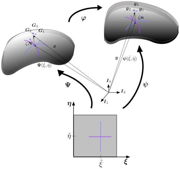
Shell kinematics. The reference mid surface is described by the embedding x = Ψ(ξ) while the deformed mid-surface is described by y = ψ(ξ). In the neighborhood of the mid surface the corresponding metrics G_i and g_i are defined for the reference and deformed configurations and the relationship between the two is the gradient of the deformation ϕ.

When employing Kirchhoff-Love kinematics, the normal to the reference mid-surface remains normal as the membrane deforms and the thickness director is inextensible. The particles of the deformed membrane can be located using only a displacement vector u from the reference mid-surface into the deformed mid-surface,

$$\mathit{y}=\varphi \left(\mathit{x}\right)=\Psi \left(\xi \right)+\mathit{u}\left(\xi \right)+\zeta \mathit{n}\left(\xi \right).$$ (9)

The surfaces are constructed using NURBS surfaces patches such that,

$$\begin{array}{cc}\hfill \mathit{x}& =R_a\left(\xi \right){\mathit{x}}_s^a+\zeta \mathit{N}\hfill \\ \hfill \mathit{y}& =R_a\left(\xi \right)({\mathit{x}}_s^a+{\mathit{u}}_s^a)+\zeta \mathit{n},\hfill \end{array}$$ (10)

where the R_a are the NURBS surface basis functions and ${\mathit{x}}_s^a,{\mathit{x}}_s^a+{\mathit{u}}_s^a$ are the corresponding control points. We note that in the previous equations and further on, we use of the summation convention, where latin indices take the values {1, 2, 3} and greek indices take values {1, 2}. We use curvilinear coordinates to locally describe the geometry. The basis vectors at every point of the reference surface are

$$\begin{array}{cc}\hfill {\mathit{E}}_1& =R_{a,\xi }{\mathit{x}}_s^a\hfill \\ \hfill {\mathit{E}}_2& =R_{a,\eta }{\mathit{x}}_s^a,\hfill \end{array}$$ (11)

and those at the deformed mid surface are

$$\begin{array}{cc}\hfill {\mathit{e}}_1& =R_{a,\xi }{\mathit{x}}_s^a+R_{a,\xi }{\mathit{u}}_s^a\hfill \\ \hfill {\mathit{e}}_2& =R_{a,\eta }{\mathit{x}}_s^a+R_{a,\eta }{\mathit{u}}_s^a.\hfill \end{array}$$ (12)

The comma indicates the partial differentiation. The dual basis satisfies e^α · e_β = ${\delta }_{\beta }^{\alpha }$, E^α · E_β = ${\delta }_{\beta }^{\alpha }$, such that the normal is a function of the surface basis vectors,

$$\mathit{N}=\frac{{\mathit{E}}_1\times {\mathit{E}}_2}{\parallel {\mathit{E}}_1\times {\mathit{E}}_2\parallel }\text{and}\mathit{n}=\frac{{\mathit{e}}_1\times {\mathit{e}}_2}{\parallel {\mathit{e}}_1\times {\mathit{e}}_2\parallel }.$$ (13)

To describe local deformations, we consider the reference metric, which consists of the covariant basis vectors in the neighborhood of the mid-surface

$$\begin{array}{cc}\hfill {\mathit{G}}_1& =R_{a,\xi }{\mathit{x}}_s^a+\zeta \frac{\partial \mathit{N}}{\partial \xi },\hfill \\ \hfill {\mathit{G}}_2& =R_{a,\eta }{\mathit{x}}_s^a+\zeta \frac{\partial \mathit{N}}{\partial \eta },\hfill \\ \hfill {\mathit{G}}_2& =\mathit{N}.\hfill \end{array}$$ (14)

The dual basis of the metric satisfies Gⁱ · G_j = δⁱ. The deformed metric is constructed in the same fashion with the corresponding covariant basis vectors near the deformed mid-surface,

$$\begin{array}{cc}\hfill {\mathit{g}}_1& =R_{a,\xi }{\mathit{x}}_s^a+R_{a,\xi }{\mathit{u}}_s^a+\zeta \frac{\partial \mathit{n}}{\partial \xi },\hfill \\ \hfill {\mathit{g}}_2& =R_{a,\eta }{\mathit{x}}_s^a+R_{a,\eta }{\mathit{u}}_s^a+\zeta \frac{\partial \mathit{n}}{\partial \eta },\hfill \\ \hfill {\mathit{g}}_3& =\mathit{n}.\hfill \end{array}$$ (15)

At this point we have completely defined the kinematics of the reference and deformed surfaces as function of the coordinates $\widehat{\xi }$ and the kinematics in the neighborhood of the corresponding mid-surfaces. Now the relationship between the reference and deformed metrics follows from using the chain rule,

$${\mathit{g}}_i=\frac{\partial \varphi \left(\mathit{x}\right)}{\partial \mathit{x}}\cdot \frac{\partial \mathit{x}}{\partial {\widehat{\xi }}^i}=\mathit{F}\cdot {\mathit{G}}_i,$$ (16)

where F is the total deformation gradient with

$$\mathit{F}={\mathit{g}}_i\otimes {\mathit{G}}^i.$$ (17)

The deformation gradient is the key kinematic quantity as it encodes the local deformation of the body. For the constitutive models in Section 4, it proofs convenient to additively decompose the total deformation gradient F,

$$\mathit{F}={\mathit{F}}_S+{\mathit{F}}_N,$$ (18)

where F_S and F_N denote the surface and normal contributions,

$${\mathit{F}}_S={\mathit{g}}_{\alpha }\otimes {\mathit{G}}^{\alpha }\text{and}{\mathit{F}}_N={\lambda }_N\mathit{n}\otimes \mathit{N}.$$ (19)

We can understand the surface deformation gradient F_S as the surface projection of the total deformation gradient F by means of the surface unit tensor I_S,

$${\mathit{F}}_S=\mathit{F}\cdot {\mathit{I}}_S\text{with}{\mathit{I}}_S=\mathit{I}-\mathit{N}\otimes \mathit{N}={\mathit{G}}_{\alpha }\otimes {\mathit{G}}^{\alpha }.$$ (20)

The surface unit tensor I_S allows us to introduce the pseudo inverse of the surface deformation gradient ${\mathit{F}}_S^{-1}$ as

$${\mathit{F}}_S^{-1}\cdot {\mathit{F}}_S={\mathit{I}}_S\text{with}{\mathit{F}}_S^{-1}={\mathit{G}}_{\alpha }\otimes {\mathit{g}}^{\alpha }.$$ (21)

Similarly, we decompose the right Cauchy Green deformation tensor,

$$\mathit{C}={\mathit{F}}^T\cdot \mathit{F}={\mathit{C}}_S+{\mathit{C}}_N,$$ (22)

into surface and normal contributions,

$${\mathit{C}}_S={\mathit{F}}_S^T\cdot {\mathit{F}}_S\text{and}{\mathit{C}}_N={\mathit{C}}_N\mathit{N}\otimes \mathit{N},$$ (23)

where the normal contribution, ${\mathit{C}}_N={\lambda }_N^2$, is equivalent to the squared stretch in thickness direction λ_N. The inverse of the right Cauchy Green surface deformation tensor, ${\mathit{C}}_S^{-1}={\mathit{F}}_S^{-1}\cdot {\mathit{F}}_S^{-T}$, follows in terms of the pseudo inverse of the surface deformation gradient ${\mathit{F}}_S^{-1}$ defined in eq. (21). We can then introduce the corresponding invariants. For the total right Cauchy Green deformation tensor, we adopt the standard definitions,

$$I_1=\mathit{C}:\mathit{I}{I}_3=\text{det}\left(\mathit{C}\right)I_4=\mathit{C}:\mathit{A}\otimes \mathit{A},$$ (24)

where the vector A belongs to the tangent space spanned by G_α and denotes the local direction of material anisotropy. For the surface right Cauchy Green deformation tensor, we use the following generalized definitions,

$$I_{S1}={\mathit{C}}_S:{\mathit{I}}_S{I}_{S3}=\widehat{det}\left({\mathit{C}}_S\right)I_{S4}={\mathit{C}}_S:\mathit{A}\otimes \mathit{A},$$ (25)

such that I₁ = I_S1 + C_N and I₄ = I_S4. To calculate the determinant of the surface deformation tensor associated with the tangent space of the surface, $\widehat{\text{det}}\left({\mathit{C}}_S\right)$, we adopt the following generalized relation [20],

$$\widehat{det}\left({\mathit{C}}_S\right)=\frac{\parallel {\mathit{g}}_1\times {\mathit{g}}_2{\parallel }^2}{\parallel {\mathit{G}}_1\times {\mathit{G}}_2{\parallel }^2}.$$ (26)

Finally, we decompose the Green Lagrange strain tensor,

$$\mathit{E}=\frac{1}{2}[{\mathit{F}}^T\cdot \mathit{F}-\mathit{I}]={\mathit{E}}_S+{\mathit{E}}_N$$ (27)

into surface strains E_S and normal strains E_N with

$${\mathit{E}}_S=({\mathit{g}}_{\alpha }\cdot {\mathit{g}}_{\beta }-{\mathit{G}}_{\alpha }\cdot {\mathit{G}}_{\beta }){\mathit{G}}^{\alpha }\otimes {\mathit{G}}^{\beta }\text{and}{\mathit{E}}_N=E_N\mathit{N}\otimes \mathit{N},$$ (28)

with the normal contribution $E_N=\frac{1}{2}[C_N-1]=\frac{1}{2}[{\lambda }_N^2-1]$.

3.2. Principle of virtual work

The internal virtual work in the reference configuration is,

$$\delta W_{int}={\int }_{B_0}\mathit{S}:\delta \mathit{E}\mathrm{dV},$$ (29)

where S is the second Piola Kirchhoff stress tensor, E is the Green Lagrange strain tensor, and δE is the variation of E with respect to the virtual displacement vector δu,

$$\delta \mathit{E}=D\left(\mathit{E}\right)\left[\delta \mathit{u}\right]=\frac{\mathrm{d}}{\mathrm{d}∊}\mathit{E}(\mathit{x}+∊\delta \mathit{u}){\mid }_{∊=0}.$$ (30)

We begin by considering the variation of the deformed metric basis vectors. The variation of the covariant basis vectors yields

$$\begin{array}{cc}\hfill \delta {\mathit{g}}_1^a& =D\left({\mathit{g}}_1\right)\left[\delta {\mathit{u}}_s^a\right]=R_{a,\xi }\delta {\mathit{u}}_s^a+\zeta D(\partial \mathit{n}∕\partial \xi )\left[\delta {\mathit{u}}_s^a\right]\hfill \\ \hfill \delta {\mathit{g}}_2^a& =D\left({\mathit{g}}_2\right)\left[\delta {\mathit{u}}_s^a\right]=R_{a,\eta }\delta {\mathit{u}}_s^a+\zeta D(\partial \mathit{n}∕\partial \eta )\left[\delta {\mathit{u}}_s^a\right]\hfill \\ \hfill \delta {\mathit{g}}_3^a& =D\left({\mathit{g}}_3\right)\left[\delta {\mathit{u}}_s^a\right]=D\left(\mathit{n}\right)\left[\delta {\mathit{u}}_s^a\right].\hfill \end{array}$$ (31)

The variation of the normal and the normal derivatives benefits from a more detailed discussion. We have avoided the use of common objects of surface differential geometry, such as the second fundamental form, to keep a strain notation that is amenable to the constitutive laws for biological materials. The constitutive equations we will encounter often appear in terms of the invariants of E. Following this reasoning, the normal derivatives can be expressed in terms of the surface covariant basis vectors,

$$\frac{\partial \mathit{n}}{\partial \xi }=\frac{\partial \mathit{n}}{\partial {\mathit{e}}_{\alpha }}\cdot \frac{\partial {\mathit{e}}_{\alpha }}{\partial \xi }\text{and}\frac{\partial \mathit{n}}{\partial \eta }=\frac{\partial \mathit{n}}{\partial {\mathit{e}}_{\alpha }}\cdot \frac{\partial {\mathit{e}}_{\alpha }}{\partial \eta }.$$ (32)

The variation of the normal follows from using the chain rule,

$$D\left(\mathit{n}\right)\left[\delta {\mathit{u}}_s^a\right]=\frac{\partial \mathit{n}}{\partial {\mathit{e}}_{\alpha }}\cdot D\left({\mathit{e}}_{\alpha }\right)\left[\delta {\mathit{u}}_s^a\right].$$ (33)

The variation of the surface base vectors takes the following simple form,

$$\begin{array}{cc}\hfill D\left({\mathit{e}}_1\right)\left[\delta {\mathit{u}}_s^a\right]& =R_{a,\xi }\delta {\mathit{u}}_s^a\hfill \\ \hfill D\left({\mathit{e}}_2\right)\left[\delta {\mathit{u}}_s^a\right]& =R_{a,\eta }\delta {\mathit{u}}_s^a.\hfill \end{array}$$ (34)

The variation of the normal derivatives can be obtained similarly through the chain rule,

$$D\left(\frac{\partial \mathit{n}}{\partial \xi }\right)\left[\delta {\mathit{u}}_s^a\right]=D\left(\frac{\partial \mathit{n}}{\partial {\mathit{e}}_{\alpha }}\right)\left[\delta {\mathit{u}}_s^a\right]\cdot \frac{\partial {\mathit{e}}_{\alpha }}{\partial \xi }+\frac{\partial \mathit{n}}{\partial {\mathit{e}}_{\alpha }}\cdot D\left(\frac{\partial {\mathit{e}}_{\alpha }}{\partial \xi }\right)\left[\delta {\mathit{u}}_s^a\right]$$ (35)

$$D\left(\frac{\partial \mathit{n}}{\partial \eta }\right)\left[\delta {\mathit{u}}_s^a\right]=D\left(\frac{\partial \mathit{n}}{\partial {\mathit{e}}_{\alpha }}\right)\left[\delta {\mathit{u}}_s^a\right]\cdot \frac{\partial {\mathit{e}}_{\alpha }}{\partial \eta }+\frac{\partial \mathit{n}}{\partial {\mathit{e}}_{\alpha }}\cdot D\left(\frac{\partial {\mathit{e}}_{\alpha }}{\partial \eta }\right)\left[\delta {\mathit{u}}_s^a\right],$$ (36)

with

$$D\left(\frac{\partial \mathit{n}}{\partial {\mathit{e}}_{\alpha }}\right)\left[\delta {\mathit{u}}_s^a\right]=\frac{{\partial }^2\mathit{n}}{\partial {\mathit{e}}_{\beta }\partial {\mathit{e}}_{\alpha }}\cdot D\left({\mathit{e}}_{\beta }\right)\left[\delta {\mathit{u}}_s^a\right]$$ (37)

and

$$\begin{array}{cc}\hfill D\left(\frac{\partial {\mathit{e}}_1}{\partial \xi }\right)\left[\delta {\mathit{u}}_s^a\right]& =R_{a,\xi \xi }\delta {\mathit{u}}_s^a\hfill \\ \hfill D\left(\frac{\partial {\mathit{e}}_1}{\partial \eta }\right)\left[\delta {\mathit{u}}_s^a\right]& =R_{a,\xi \eta }\delta {\mathit{u}}_s^a=D\left(\frac{\partial {\mathit{e}}_2}{\partial \xi }\right)\left[\delta {\mathit{u}}_s^a\right]\hfill \\ \hfill D\left(\frac{\partial {\mathit{e}}_2}{\partial \eta }\right)\left[\delta {\mathit{u}}_s^a\right]& =R_{a,\eta \eta }\delta {\mathit{u}}_s^a.\hfill \end{array}$$ (38)

With variation of the deformation gradient,

$$\delta \mathit{F}=\delta {\mathit{g}}_i\otimes {\mathit{G}}^i,$$ (39)

the desired variation of the Green Lagrange strain tensor is readily computed,

$$\delta \mathit{E}=\frac{1}{2}(\delta {\mathit{F}}^T\mathit{F}+{\mathit{F}}^T\delta \mathit{F}).$$ (40)

3.3. Consistent linearization

To solve the resulting nonlinear system we require the linearization of the internal virtual work,

$$D\left(\delta W_{int}\right)[\Delta \mathit{u}]={\int }_{B_0}D\mathit{E}:\mathbb{ℂ}:\delta \mathit{E}\mathrm{dV}+{\int }_{B_0}\mathit{S}:D\delta \mathit{E}\mathrm{dV}.$$ (41)

Here, $\mathbb{ℂ}$ denotes the material fourth order elasticity tensor $\mathbb{ℂ}$ = ∂S/∂E. The linearization is done with the directional derivative D(•)[Δu] defined above (30). The linearization DE is essentially the same as the first variation δE but now in the direction of the increment Δu. The linearization of the first variation, DδE, consists of four terms,

$$D\delta \mathit{E}=\frac{1}{2}(\delta {\mathit{F}}^{T}D\mathit{F}+D{\mathit{F}}^T\delta \mathit{F}+D\delta {\mathit{F}}^T\mathit{F}+{\mathit{F}}^{T}D\delta \mathit{F}),$$ (42)

including the second variation of the deformed metric,

$$D\delta \mathit{F}=D\delta {\mathit{g}}_i\otimes {\mathit{G}}^i,$$ (43)

which requires the second directional derivatives of the deformed metric basis vectors,

$$\begin{array}{cc}\hfill D\delta {\mathit{g}}_1^{ab}& =D^2(\partial \mathit{n}∕\partial \xi )[\delta {\mathit{u}}_s^a,\Delta {\mathit{u}}_s^b]\hfill \\ \hfill D\delta {\mathit{g}}_2^{ab}& =D^2(\partial \mathit{n}∕\partial \eta )[\delta {\mathit{u}}_s^a,\Delta {\mathit{u}}_s^b]\hfill \\ \hfill D\delta {\mathit{g}}_3^{ab}& =D^2\left(\mathit{n}\right)[\delta {\mathit{u}}_s^a,\Delta {\mathit{u}}_s^b].\hfill \end{array}$$ (44)

Since the linearization of all variations in (38) vanishes, we only need to include the linearization of (37),

$$D^2\left(\frac{\partial \mathit{n}}{\partial {\mathit{e}}_{\alpha }}\right)[\delta {\mathit{u}}_s^a,\Delta {\mathit{u}}_s^b]=\frac{{\partial }^3\mathit{n}}{\partial {\mathit{e}}_{\gamma }\partial {\mathit{e}}_{\beta }\partial {\mathit{e}}_{\alpha }}:\left(D\left({\mathit{e}}_{\beta }\right)\left[\delta {\mathit{u}}_s^a\right]\otimes D\left({\mathit{e}}_{\gamma }\right)[\Delta {\mathit{u}}_s^b]\right).$$ (45)

4. Constitutive equations

So far, we have kept the principle of virtual work for a three-dimensional solid in an effort to keep our derivations as general as possible before choosing a specific constitutive equation. In this setting we are unable to perform an explicit integration of the residual forces through the thickness to obtain resulting forces and moments in terms of the first and second fundamental forms of the midsurface, a common procedure when deriving thin shell formulations [31].

When modeling biological materials, constitutive laws such as the St. Venant-Kirchhoff model may not be the best choice to accurately capture the mechanical behavior of the tissues under large deformations. When biological membranes undergo large physiological deformations they require constitutive laws that recreate a complex relationship between stresses and strains that is highly nonlinear and anisotropic [16]. Determining appropriate constitutive equations for soft biological materials is a problem on its own that has drawn significant attention [42]. Early work on the modeling of blood vessels employed isotropic strain energy potentials of the Mooney-Rivlin type. However, it is now commonly accepted that transverse isotropic descriptions are more appropriate. Most soft tissues have a well defined microstructure characterized by the presence of fibers such as collagen. The preferred orientation of these fiber bundles, which is responsible for tissue anisotropy has been incorporated in more recent constitutive models [24]. When exploring constitutive laws for membranes we can take two alternative approaches: we can either establish reduced two-dimensional constitutive equations dependent on the inplane deformation only or adapt a fully three-dimensional strain energy function for solids and enforce plane stress conditions. Here we focus on the second approach. To show the flexibility of our formulation, we briefly discuss four constitutive models that can be easily embedded within our framework. Many other constitutive models can be adapted in a similar way. In general, for arbitrary, nonlinear constitutive models, it is always possible to iteratively determine the normal strain that satisfies the plane stress condition [35].

4.1. St. Venant Kirchhoff model

Although the expression for the stress of the St. Venant Kirchhoff (VK) material adjusted to thin membranes is well known, we briefly illustrate the derivation starting from the three-dimensional strain energy function to show that we indeed have an identical formulation to the one in the literature [31] before the explicit integration across the thickness. The strain energy function is

$$\psi =\frac{1}{2}\lambda \left(\text{tr}\mathit{E}\right)+\mu \mathit{E}:\mathit{E},$$ (46)

from which the second Piola Kirchhoff stress tensor follows,

$$\mathit{S}=\frac{\partial \psi }{\partial \mathit{E}}=\lambda \left(\text{tr}\mathit{E}\right)\mathit{I}+2\mu \mathit{E}.$$ (47)

To satisfy the plane stress condition, we consider the Green Lagrange strain tensor as the sum of the surface strain and the normal strain, E = E_S + E_N. Then the stress follows a similar additive decomposition,

$$\mathit{S}={\mathit{S}}_S+{\mathit{S}}_N,$$ (48)

in terms of the surface and normal contributions,

$$\begin{array}{cc}\hfill {\mathit{S}}_S& =\lambda ({\mathit{E}}_S:{\mathit{I}}_S+E_N){\mathit{I}}_S+2\mu {\mathit{E}}_S\hfill \\ \hfill {\mathit{S}}_B& =\lambda ({\mathit{E}}_S:{\mathit{I}}_S+E_N)\mathit{N}\otimes \mathit{N}+2\mu {\mathit{E}}_N.\hfill \end{array}$$ (49)

By setting the normal stress to zero, S_N = λ(E_S : I_S ) + (λ + 2μ) E_N ≐ 0, we obtain an explicit expression for the normal strain E_N in terms of the surface strain E_S,

$$E_N=\frac{-\lambda }{\lambda +2\mu }({\mathit{E}}_S:{\mathit{I}}_S),$$ (50)

which we substitute back into the definition of the surface stress in eq. (49),

$${\mathit{S}}_S=\frac{2\mu \lambda }{\lambda +2\mu }({\mathit{E}}_S:{\mathit{I}}_S){\mathit{I}}_S+2\mu {\mathit{E}}_S.$$ (51)

In the small-strain limit, we can express the Lamé constants λ and μ in terms of the Young’s modulus E and Poisson’s ratio ν,

$${\mathit{S}}_S=\frac{E\nu }{1-{\nu }^2}({\mathit{E}}_S:{\mathit{I}}_S){\mathit{I}}_S+\frac{E}{1+\nu }{\mathit{E}}_S,$$ (52)

which is the final expression for the stress as function of the surface deformation, equivalent to the literature [31]. The material tangent follows from using the chain rule,

$$\mathbb{ℂ}=\frac{\partial \mathit{S}}{\partial \mathit{E}}=\frac{\partial \mathit{S}}{\partial {\mathit{E}}_S}:\frac{\partial {\mathit{E}}_S}{\partial \mathit{E}}.$$ (53)

The first term is straightforward to compute,

$${\mathbb{ℂ}}_S=\frac{\partial \mathit{S}}{\partial {\mathit{E}}_S}=\frac{2\mu \lambda }{\lambda +2\mu }{\mathit{I}}_S\otimes {\mathit{I}}_S+2\mu {\mathbb{𝕀}}_S,$$ (54)

where ${\mathbb{𝕀}}_S$ is the fourth order identity tensor of the surface tangent space. The second term,

$$\frac{\partial {\mathit{E}}_S}{\partial \mathit{E}}=\frac{\partial (\mathit{E}-E_N\mathit{N}\otimes \mathit{N})}{\partial \mathit{E}}=\mathbb{𝕀}+\frac{\lambda }{\lambda +2\mu }\mathit{N}\otimes \mathit{N}\otimes {\mathit{I}}_S,$$ (55)

accounts for the fact that the surface and normal strains are related to satisfy the plane stress condition. Here we have used the fact that the projection, I_S : ∂E_S/∂E = I_S, is equivalent to the surface unit tensor. Contracting ${\mathbb{ℂ}}_S$ with ∂E_S/∂E in eq. (53) has no effect, and $\mathbb{ℂ}\equiv {\mathbb{ℂ}}_S$.

4.2. Mooney-Rivlin model

Mooney Rivlin (MR) constitutive equations, often used to describe rubber materials, were amongst the first choices to model arteries and other biomembranes [29]. The three-dimensional strain energy function of Mooney Rivlin type, supplemented by a contribution in the fiber direction, is

$$\psi =\mu [(I_1-3)+\alpha (I_2-3)+\beta {(I_4-1)}^2].$$ (56)

Here we introduce the Mooney Rivlin potential to model orthotropic membranes directly in terms of the surface strains [36]. This formulation applies to some biological structures such as cell membranes or soft tissues at low strain regimes [45]. We reformulate the strain energy function in terms of the surface invariants defined in eq. (25),

$${\psi }_S=\mu [(I_{IS}+I_{S3}^{-1}-3)+\alpha (I_{S3}+I_{S1}{I}_{S3}^{-1}-3)+\beta {(I_{S4}-1)}^2].$$ (57)

We obtain the second Piola Kirchhoff surface stress S_S as

$${\mathit{S}}_S=2\frac{\partial {\psi }_S}{\partial {\mathit{C}}_S}=2\mu [(1-\alpha I_{S3}^{-1}){\mathit{I}}_S+(\alpha (I_{S3}-I_{S1}{I}_{S3}^{-1})-I_{S3}^{-1}){\mathit{C}}_S^{-1}+2\beta I_{S4}\mathit{A}\otimes \mathit{A}],$$ (58)

and the corresponding surface tangent moduli as,

$$\begin{array}{cc}\hfill {\mathbb{ℂ}}_S=2\frac{\partial {\mathit{S}}_S}{\partial {\mathit{C}}_S}=4\mu [& (\alpha (I_{S3}-I_{S1}{I}_{S3}^{-1})+I_{S3}^{-1}){\mathit{C}}_S^{-1}\otimes {\mathit{C}}_S^{-1}\hfill \\ \hfill & +(\alpha I_{3S}-I_{S3}^{-1}-\alpha I_{S1}{I}_{S3}^{-1})\frac{\partial {\mathit{C}}_S^{-1}}{\partial {\mathit{C}}_S}\hfill \\ \hfill & -\alpha I_{S3}^{-1}({\mathit{I}}_S\otimes {\mathit{C}}_S^{-1}+{\mathit{C}}_S^{-1}\otimes {\mathit{I}}_S)\hfill \\ \hfill & +2\beta \mathit{A}\otimes \mathit{A}\otimes \mathit{A}\otimes \mathit{A}].\hfill \end{array}$$ (59)

4.3. May-Newman-Yin model

Constitutive equations for cardiac tissues have received special attention. This is not surprising – heart valves, for example, are obvious examples of biological membranes with crucial mechanical roles in the human body. The seminal work by May-Newman and Yin (MY) introduced a constitutive law with an exponential contribution to the strain energy that was used successfully to model heart valves under biaxial tests [38]. More recent work by Prot and Holzapfel modified the strain energy function proposed by May-Newman and Yin and used it to explore more realistic out-of-plane deformations while, at the same time, imposing incompressibility [40]. Here we revisit the latter implementation within our formulation. Its strain energy function is

$$\psi =c_0[\text{exp}(c_1{(I_1-3)}^2+c_2{(I_4-1)}^2)-1].$$ (60)

To impose incompressibility, we adopt a Lagrange multiplier approach,

$$\widehat{\psi }=c_0[\text{exp}(c_1{(I_1-3)}^2+c_2{(I_4-1)}^2)-1]+p(J-1).$$ (61)

The second Piola Kirchhoff stress tensor follows as

$$\mathit{S}=2\frac{\partial \widehat{\psi }}{\partial \mathit{C}}=2{\psi }_1\mathit{I}+2{\psi }_4\mathit{A}\otimes \mathit{A}+2p{\mathit{C}}^{-1}.$$ (62)

Here ψ_i = ∂ψ/∂I_i denotes the derivatives of the strain energy function with respect to the first and fourth invariants of C. We adopt the additive decomposition of the right Cauchy Green strain tensor into surface and normal contributions,C = C_S + C_N . We solve for the pressure to satisfy the plane stress condition and calculate the normal strain component explicitly using the incompressibility constraint,

$$p=-2{\psi }_1{C}_N\text{with}{C}_N=1∕I_{S3}.$$ (63)

After substituting I₁ = I_S1 + C_N and I₄ = I_S4 in the expressions for ψ_i, the stress in eq. (62) is now only a function of the surface strain invariants,

$$\mathit{S}={\mathit{S}}_S=2{\psi }_1{\mathit{I}}_S+2{\psi }_4\mathit{A}\otimes \mathit{A}-2{\psi }_1∕I_{S3}{\mathit{C}}_S^{-1}.$$ (64)

The tangent moduli follow as

$$\mathbb{ℂ}=2\frac{\partial \mathit{S}}{\partial \mathit{C}}=2\frac{\partial {\mathit{S}}_S}{\partial {\mathit{C}}_S}:\frac{\partial {\mathit{C}}_S}{\partial \mathit{C}}.$$ (65)

The first term denotes the surface tangent moduli,

$$\begin{array}{cc}\hfill {\mathbb{ℂ}}_S& =2\frac{\partial {\mathit{S}}_S}{\partial {\mathit{C}}_S}\hfill \\ \hfill & =2{\psi }_{11}{\mathit{I}}_S\otimes {\mathit{I}}_S+2{\psi }_{14}({\mathit{I}}_S\otimes \mathit{A}\otimes \mathit{A}+\mathit{A}\otimes \mathit{A}\otimes {\mathit{I}}_S)\hfill \\ \hfill & +2{\psi }_{44}\mathit{A}\otimes \mathit{A}\otimes \mathit{A}\otimes \mathit{A}-2{\psi }_{11}{I}_{S3}^{-1}{\mathit{C}}_S^{-1}\otimes {\mathit{I}}_S\hfill \\ \hfill & -2{\psi }_{14}{I}_{S3}^{-1}{\mathit{C}}_S^{-1}\otimes \mathit{A}\otimes \mathit{A}\hfill \\ \hfill & +2{\psi }_1{I}_{S3}^{-1}({\mathit{C}}_S^{-1}\otimes {\mathit{C}}_S^{-1}-\frac{\partial {\mathit{C}}_S^{-1}}{\partial {\mathit{C}}_S}),\hfill \end{array}$$ (66)

where the abbreviation ψ_ij denotes the second derivatives of the strain energy with respect to the surface invariants, ψ_ij = ∂ψ_i/∂I_Sj. The second term is

$$\frac{\partial {\mathit{C}}_S}{\partial \mathit{C}}=\mathbb{𝕀}-C_N\mathit{N}\otimes \mathit{N}\otimes \mathit{N}\otimes \mathit{N}.$$ (67)

Contracting ${\mathbb{ℂ}}_S$ with ∂C_S/∂C in eq. (65) has no effect, and $\mathbb{ℂ}\equiv {\mathbb{ℂ}}_S$.

4.4. Gasser-Ogden-Holzapfel model

Originally developed to model arteries, the strain energy function proposed by Gasser, Ogden and Holzapfel (GOH), has been readily adopted to model other thin biological tissues with a well-defined microstructure such as skin [1, 17]. This constitutive law accounts for an isotropic response due to the water-based matrix, and an exponential contribution from a distributed family of fibers. While the original model assumes a three-dimensional fiber dispersion function, in thin biological membranes, fibers lie primarily within the plane, and a two-dimensional fiber dispersion function seems appropriate [12]. The strain energy function then becomes a sum of a three-dimensional Neo-Hookean contribution, plus an exponential term from a two dimensional fiber family,

$$\psi =c(I_1-3)+\frac{k_1}{2k_2}\text{exp}\left[k_2{(\kappa I_{S1}+(1-2\kappa )I_{S4}-1])}^2\right]-1.$$ (68)

Again, we impose incompressibility using a Lagrange multiplier approach,

$$\widehat{\psi }=c(I_1-3)+\frac{k_1}{{2_K}_2}\text{exp}\left[k_2{(\kappa I_{S1}+(1-2\kappa )I_{S4}-1])}^2\right]-1+p(J-1).$$ (69)

The second Piola Kirchhoff stress tensor is

$$\mathit{S}=2\frac{\partial \widehat{\psi }}{\partial \mathit{C}}=2c\mathit{I}+2{\psi }_1{\mathit{I}}_S:\frac{\partial {\mathit{C}}_S}{\partial \mathit{C}}+2{\psi }_4\mathit{A}\otimes \mathit{A}+2p{\mathit{C}}^{-1},$$ (70)

where ψ_i = ∂ψ/∂I_{S i} denotes the derivative of the strain energy function with respect to the first and fourth surface invariants of C_S . The decomposition of the right Cauchy Green deformation tensor into surface and normal contributions allows us to explicitly define the pressure p using the incompressibility constraint,

$$p=-c{C}_N\text{with}{C}_N=1∕I_{S3}.$$ (71)

The derivative of the surface deformation tensor with respect to the total deformation tensor is

$$\frac{\partial {\mathit{C}}_S}{\partial \mathit{C}}=\mathbb{𝕀}+C_N\mathit{N}\otimes \mathit{N}\otimes \mathit{N}\otimes \mathit{N},$$ (72)

and the second Piola Kirchhoff stress that satisfies the plane stress condition reduces to the following expression,

$$\mathit{S}={\mathit{S}}_S=2c\mathit{I}+2{\psi }_1{\mathit{I}}_S+2{\psi }_4\mathit{A}\otimes \mathit{A}-2c{I}_{S3}^{-1}{\mathit{C}}^{-1}.$$ (73)

The tangent moduli for this constitutive law are

$$\begin{array}{cc}\hfill {\mathbb{ℂ}}_S& =4{\psi }_{11}{\mathit{I}}_S\otimes {\mathit{I}}_S+4{\psi }_{14}({\mathit{I}}_S\otimes \mathit{A}\otimes \mathit{A}+\mathit{A}\otimes \mathit{A}\otimes {\mathit{I}}_S)\hfill \\ \hfill & +4{\psi }_{44}\mathit{A}\otimes \mathit{A}\otimes \mathit{A}\otimes \mathit{A}+4c{I}_{S3}^{-1}({\mathit{C}}_S^{-1}\otimes {\mathit{C}}_S^{-1}-\frac{\partial {\mathit{c}}_S^{-1}}{\partial {\mathit{C}}_S}),\hfill \end{array}$$ (74)

where the abbreviation ψ_{i j} denotes the second derivatives of the strain energy with respect to the surface invariants, ψ_{i j} = ∂ψ_i/∂I_{S j}.

5. Examples

5.1. In-plane biaxial tests

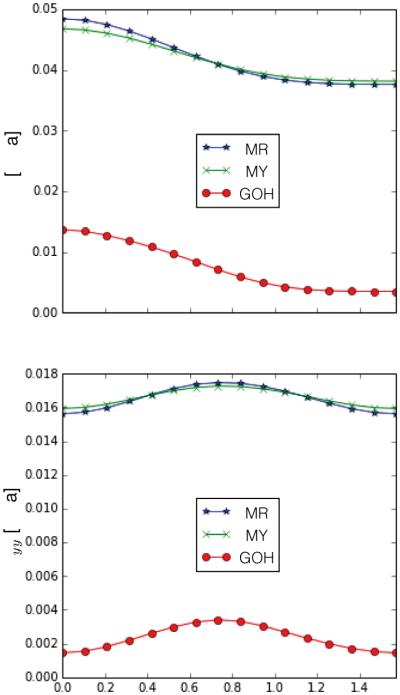
To probe the correct implementation of the four material subroutines outlined before, we perform simple strip-biaxial tests. We use the material parameters indicated in Table 1. The parameters for the GOH model are taken from skin tissue simulations and the remaining parameters were obtained by a simple numerical fit of three biaxial testing scenarios [9]. In all cases we start with a square geometry of unit size parametrized with quadratic B-splines and knot vectors Ξ = Ω = [0, 0, 0, 0.25, 0.5, 0.75, 1, 1, 1] and impose final principal stretches λ_x = 1.2, λ_y = 1.0. Plots of the Cauchy stresses σ_xx and σ_yy for varying λ_x are depicted in Figure 2 for each material. For the anisotropic constitutive laws, we employ A = G₁ which coincides with the x coordinate axis. The materials exhibit mild nonlinearity. We obtain homogeneous deformations and the curves match the theoretical results, which provides confidence in the implementation of the element, the constitutive law, and the corresponding tangent moduli.

Table 1.

Material parameters for the different constitutive laws.

Const. Law	Parameters
VK	μ = 1.59 × 10−2MPa, λ = 51.63
MR	μ = 0.0245MPa, 0.0245MPa, α = 0.0297, β = 0.347
MY	c0 = 5.95MPa, c1 = 1.48 × 10−3MPa, c2 = 6.74× 10−4
GOH	c = .0511MPa, k1 = 0.015MPa, k2 = 0.0418, κ = 0.05

Figure 2.

Strip biaxial test for the four different constitutive equations outlined: VK, MR, MY and GOH. The original geometry is a square discretized with 6 × 6 elements mesh. While the sample is fixed in the y direction, a displacement is gradually applied in the x direction. The simulations yield a homogeneous deformation which agrees with the theoretical result. The materials exhibit mild nonlinearity, particularly for the MY model it is evident the influence of the exponential term as the strain increases.

For the anisotropic materials, Figure 3 shows the variation of σ_xx and σ_yy at (x, y) = (0.5, 0.5) for λ_x = 1.20 obtained through varying θ. The angle θ corresponds to the in-plane rotation with respect to the covariant base vector G₁, thus, θ = 0 indicates a preferred stiffness direction A = G₁, here aligned with the x coordinate, and θ = π/2 corresponds to A = G₂ aligned with y axis. The anisotropic stress contribution is of the form f_I4 · A ⊗ A where f_I4 denotes a function of the stretch, I₄ of A. The largest contribution in the xx component of the stress naturally occurs when A = G₁ and contributions can only decrease for different θ. For the yy component, however, the structural tensor A ⊗ A has no contribution when A = G₁ and I₄ is maximum, and has full contribution when A = G₂, but then I₄ = 0. This interplay between the structural tensor and the stretch of A results in a bell-shaped curve with maximum σ_yy at θ = π/4.

Figure 3.

Anisotropy behavior obtained through varying the preferred direction A determined by θ, the angle with respect to G₁ . The xx component of the stress decreases while the yy component achieves its maximum at θ = π/4.

5.2. Rectangular strip subjected to end shearing force

We analyze the performance of our formulation with respect to a popular benchmark problem, a strip pulled by a shear force at its free edge [47]. The geometry consists of a rectangular shell of dimensions 10 × 1 and thickness 0.05. We first simulate the VK material with E = 1.2 × 10⁶ and ν = 0. No units are specified. The objective in this example is to compare our results to a popular benchmark problem. To impose the clamped-edge boundary condition, we adopt a method from the literature and fix the z-coordinate of the second row of control points closest to the clamped edge to fix the tangent at that edge [31]. Figure 4 shows the schematic of the problem and Figure 5 exhibits the plot of the solution and the reference values [47]. These results correspond to quadratic B-splines meshes with 25 elements along the length and 3 in across the width. The present formulation excellently matches the reference values.

Figure 4.

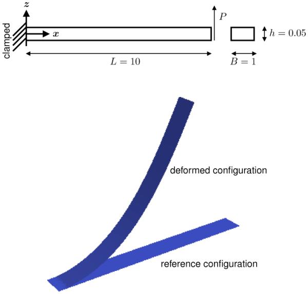
Schematic of the tip deflection example used as a popular benchmark test for thin shells. The geometry is a rectangular strip clamped at one end. A vertical shearing force is applied at the opposite end. The bottom part of the figure shows the reference geometry and the resulting deformation when the maximum load is applied.

Figure 5.

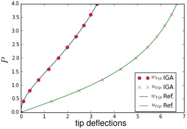
Deflections of the tip for the pulled strip subjected to end shearing force. w_tip corresponds to the displacement in the z coordinate while u_tip denotes the negative of the x displacement. The simulation results obtained with the present formulation agree well with the reference solution for a mesh of 25 × 3 elements.

To showcase the choice of other materials, we perfumed simulations for the anisotropic materials listed in Table 1. The dimension is now 10 × 1mm and the forces applied at the end are on the order of Newtons. Figure 6 shows the deflection curves when A = [1, 0, 0] for the same mesh as before consisting of 25 × 3 elements. The additional flexibility of the proposed constitutive laws to incorporate the anisotropy of non-linear materials allows to capture interesting geometric effects: For instance, we perform a similar simulation as before but in a strip of dimensions 30 × 10mm meshed with a 25 × 12 elements patch and employ the GOH model with a fiber direction oriented obliquely at θ = π/4, where θ is the angle between the anisotropy direction A and the covariant vector G₁. We impose a force of P = 0.04N. Figure 7 shows the result of the y displacement at the tip of the strip. For the isotropic material and for anisotropic materials with A aligned with G₁, the y displacement is identically zero at the free edge. Now, the inclusion of an oblique fiber direction breaks the symmetry. This is similar to heart valve leaflets, for example, where the presence of a non-trivial fiber distributions can create rich and complex deformation patterns, even for simple loading scenarios.

Figure 6.

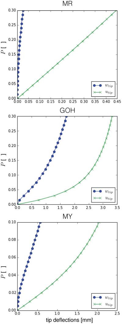
Deflections of the tip for the pulled strip using the anisotropic material models subjected to end shearing force. w_tip corresponds to the displacement in z while u_tip denotes the negative of the x displacement. Very different curves are seen for the different materials. The MY case deflects under less loading and the MR material exhibits the least deflection out of the three anisotropic models studied.

Figure 7.

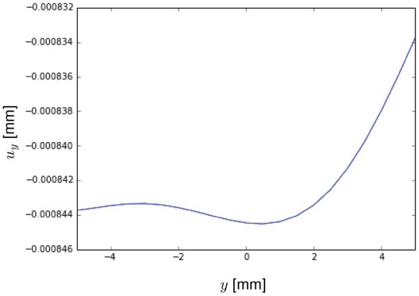
y displacement at the tip of a 30 × 10mm strip subjected to end shearing force. Unlike the isotropic case or an orthotropic membrane aligned with the loading, the presence of an oblique anisotropic direction induces more complex three-dimensional deformations. For isotropic membranes a vertical shearing force causes exactly zero y displacements, while the same loading for an anisotropic strip with oblique preferred direction results in an interesting deformation at the tip with non-zero y motion.

5.3. Inflation of a rectangular membrane

A major motivation for the present work is the application to relevant clinical problems. For instance, in plastic a reconstructive surgery, tissue expansion is a widely employed procedure that allows to ultimately grow skin in situ by imposing stretches beyond the physiological limit. In an idealized geometry, skin expansion can be viewed as the inflation of a rectangular membrane. As reference geometry, we take a square of 10 × 10cm and apply a normal pressure of 1kPa to induce out-of-plane deformation.

Figure 8 illustrates the convergence of the formulation for the MR material with parameters μ = 1, α = 0.0245, β = 0.0297, and A forming a 0.347 angle with respect to G₁. We are interested in tracking the solution upon h- and k-refinement [28]. We perform the simulation with meshes of 5, 10, 20, 40 elements per side and degrees of the B-spline basis functions 2, 3, 4. Figure 8 shows the vertical displacement at the center of the membrane. It confirms that all meshes rapidly approach the same value of 19.3112mm upon h- and k-refinement.

Figure 8.

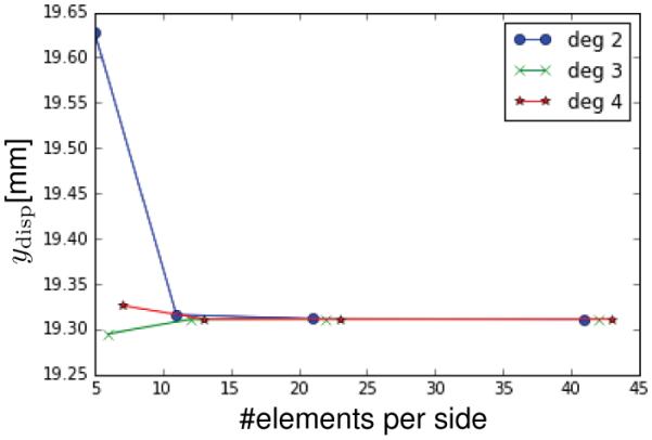
Convergence of a rectangular membrane subjected to out-of-plane pressure. The plot shows the vertical displacement of the center point of the membrane for a pressure of 1kPa for different mesh sizes and degrees of the basis functions. The resulting deformation converges rapidly upon both h and k refinement.

We are also interested in capturing the unique deformations resulting from anisotropy. A inflated rectangular membrane deforms differently in the directions parallel and perpendicular to its fiber orientation A and creates a characteristic bean shape. This is illustrated in Figure 9, where we show the four final configurations of the different materials subjected to the same pressure. We used 12 × 12 meshes of quadratic B-splines and imposed 1kPa of normal pressure. The VK material deforms isotropically turning into a spheroid, while the other three geometries exhibit marked anisotropy. Table 2 summarizes the degree of anisotropy by measuring the lengths of the XZ and YZ cross sections at the center of the membrane as a measure of ellipticity. While the coarse mesh does not capture the details of the deformation at the corners, it is capable of correctly resolving the ellipticity and the overall shape. For example, inflation of the GOH material results in an identical value of 0.68 for both the coarse mesh and the 30 × 30 mesh.

Figure 9.

Inflation of a rectangular membrane by applying a normal out-of-plane pressure. The four final configurations shown correspond to the different constitutive laws under study. The VK material exhibits an isotropic deformation while all other three reach a final state with greater deformation opposite to the preferred direction of anisotropy. Particularly the MR and GOH materials show marked bean shapes.

Table 2.

Ellipticity of inflated membranes. Applying normal pressure to a flat VK material leads to isotropic deformation while materials with preferred stiffness direction (MR, MY and GOH) lead to bean-like shapes.

Const. Law	Pressure [kPa]	Lengthxz [mm]	Lengthyz [mm]	Ellipticity [-]
VK	1	217.2	217.2	0.00
MR	1	237.3	314.0	0.65
MY	1	201.3	210.7	0.29
GOH	1	224.2	307.3	0.68

6. Discussion

We have presented a thin shell formulation based on Kirchhoff-Love kinematics and isogeometric analysis tailored for nonlinear anisotropic materials. Isogeometric analysis has been readily used to formulate thin shell elements because of its inherent C¹ continuity required for Kirchoff-Love kinematics [31]. However, with a few exceptions [11], attention has remained on linear isotropic constitutive laws. Yet, numerous research efforts have motivated constitutive equations that incorporate the highly nonlinear and markedly anisotropy behavior of biological tissues [42]. Our objective was to incorporate constitutive equations that have been specifically designed for collagenous tissues with preferred fiber orientations into the isogeometric framework of thin shells [8].

We summarized the kinematics of a thin shell using convective curvilinear coordinates. Following the Kirchhoff-Love assumptions, we imposed the constraint that the normal to the mid surface remains normal and un-stretched. We presented the weak form of the linear momentum balance for a three-dimensional solid. At this point, however, we departed from existing isogeometric thin shell models [31]. While it is common to perform explicit integration through the thickness and express the balance equations in terms of force and moment normals, here we kept the fully three-dimensional version of the equilibrium equations. This setup keeps the formulation as close as possible to the description familiar to the biomechanics community [25]. We then performed the consistent linearization with respect to the degrees of freedom. At this point our formulation remains open for the constitute model, which best suits the desired application. We remark that the integration across the thickness has to be performed numerically. Here we have followed recommendations from nonlinear shell analysis, which suggest the use of 3-point Lobatto integration for smooth integrals [26]. However, more careful considerations can become necessary; ideally, the integration scheme is adjusted to the individual deformation pattern of underlying application.

To illustrate the flexibility of the current approach, we incorporated four widely used constitutive laws: the St. Venant Kirchhoff (VK), Mooney-Rivlin (MR), May Newmann-Yin (MY) and Gasser-Ogden-Holzapfel (GOH) models. For each model, we showed how to adapted it to satisfy the plane stress condition and derived the consistent tangent moduli. This procedure is conceptually generic and can easily be adopted for other hyperelastic material models. Within the context of biological membranes, it is worth raising the question of whether a shell formulation is necessary or whether it is sufficient to consider a membrane formulation alone. If we postulate that nature optimizes form and function, it would be reasonable to assume that biological systems in vivo are loaded such that bending moments are minimized [33]. Yet, any living system can be subjected to non-physiological conditions, especially in disease, where bending stresses might become important. For example, studies of bio-prosthetic heart valves have shown how leaflets undergo significant changes in curvature leading to tissue damage over many loading cycles [18, 37]. We believe it is important to consider both–membrane and bending energies–with a thin shell description.

We analyzed selected benchmark examples to illustrate the performance of our formulation and its ability to capture the rich deformations that occur in response to material anisotropy. To demonstrate the correct implementation of the constitutive law and the corresponding tangent moduli, we analyzed the homogeneous deformation in simple strip biaxial tests. We also discussed a benchmark problem to illustrate the equivalence between the present work and the St. Venant Kirchhoff model [31]. We selected a rectangular strip subjected to a shear force at its free edge. Incorporating oblique fiber directions induced deformations that were not present in the isotropic case. We finally turned our attention to a more clinically inspired example, a clamped membrane inflated by a transverse pressure. This example resembles the process of skin expansion, a widely used reconstructive technique [6]. We demonstrated the convergence of the problem upon h- and k-refinement. For the four different materials, the final configuration under the same pressure displayed significant differences: The VK material deformed isotropically as expected. The MY material showed anisotropy, yet with a mild degree of ellipticity. The MR and GOH materials, on the contrary, generated highly anisotropic bean shape patterns. This type of deformation agrees with experimental observations. We have conducted controlled experiments of skin expansion and found significant differences in strains parallel and orthogonal to Langer’s lines, which are associated with collagen fiber orientations [10].

Here, for the sake of comparison with the literature, we have presented only simulations of simple geometries constructed from a single tensor product surface patch. To simulate complex geometries of multiples surface patches, we could adopt the bending strip method or Nitsche’s method [21, 32]. For shell geometries with sharp corners, a hybrid shell formulation with combined Kirchhoff-Love kinematics for smooth regions and Reissner-Mindlin kinematics for sharp regions has been recently proposed [5]. The efforts in this direction have proven critical for the simulation of very intricate geometries in engineering applications such as wind turbines [2].

In summary, isogeometric analysis is a powerful tool to develop shell formulations with inherent high continuity. By embedding a set constitutive models for nonlinear anisotropic materials, we hope to unleash the benefits of isogeometric analysis within the biomechanics community, in which recent research efforts have generated a library of constitutive models for soft biological tissues. Our generic framework has various natural and potentially high impact applications. In particular, we will use this model to simulate heart valve leaflets and skin deformations in cardiac and reconstructive surgery.

Highlights.

We present a thin shell formulation for thin biological membranes

We employ Isogeometric Analysis with NURBS tensor product surface patches

We present the balance equation and its linearization for arbitrary constitutive laws

We incorporate constitutive equations designed specifically for collagenous tissues

Incompressible materials lead to a closed-form solution of the plane stress condition

References

- [1].Annaidh AN, Bruyère K, Destrade M, Gilchrist MD, Maurini C, Otténio M, Saccomandi G. Automated estimation of collagen fibre dispersion in the dermis and its contribution to the anisotropic behaviour of skin. Ann Biomed Eng. 2012;40(8):1666–1678. doi: 10.1007/s10439-012-0542-3. [DOI] [PubMed] [Google Scholar]
- [2].Bazilevs Y, Hsu MC, Scott MA. Isogeometric fluid-structure interaction analysis with emphasis on non-matching discretizations, and with application to wind turbines. Comput Methods Appl Mech Eng. 2012;249:28–41. [Google Scholar]
- [3].Benson DJ, Bazilevs Y, Hsu MC, Hughes TJR. Isogeometric shell analysis: The Reissner-Mindlin shell. Comput Methods Appl Mech Eng. 2011;199:276–289. [Google Scholar]
- [4].Benson DJ, Bazilevs Y, Hsu MC, Hughes TJR. A large deformation, rotation-free, isogeometric shell. Comput Methods Appl Mech Eng. 2011;200:1367–1378. [Google Scholar]
- [5].Benson DJ, Hartmann S, Bazilevs Y, Hsu MC, Hughes TJR. Blended isogeometric shells. Comput Methods Appl Mech Eng. 2013;255:133–146. [Google Scholar]
- [6].Buganza Tepole A, Ploch CJ, Wong J, Gosain AK, Kuhl E. Growing skin - A computational model for skin expansion in reconstructive surgery. J Mech Phys Solids. 2011;59:2177–2190. doi: 10.1016/j.jmps.2011.05.004. [DOI] [PMC free article] [PubMed] [Google Scholar]
- [7].Buganza Tepole A, Gosain AK, Kuhl E. Stretching skin: The physiological limit and beyond. Int J Nonlin Mech. 2012;47:938–949. doi: 10.1016/j.ijnonlinmec.2011.07.006. [DOI] [PMC free article] [PubMed] [Google Scholar]
- [8].Buganza Tepole A, Gart M, Gosain AK, Kuhl E. Characterization of living skin using multi view stereo and isogeometric analysis. Acta Biomat. 2014;10:4822–4831. doi: 10.1016/j.actbio.2014.06.037. [DOI] [PMC free article] [PubMed] [Google Scholar]
- [9].Buganza Tepole A, Gosain AK, Kuhl E. Computational modeling of skin: Using stress profiles as predictor for tissue necrosis in reconstructive surgery. Comput Struct. 2014;143:32–39. doi: 10.1016/j.compstruc.2014.07.004. [DOI] [PMC free article] [PubMed] [Google Scholar]
- [10].Buganza Tepole A, Gart M, Purnell CA, Gosain AK, Kuhl E. Multi-view stereo analysis reveals anisotropy of prestrain, deformation, and growth in living skin. Biomech Mod Mechanobiol. 2015 doi: 10.1007/s10237-015-0650-8. doi:10.1007/s10237-015-0650-8. [DOI] [PMC free article] [PubMed] [Google Scholar]
- [11].Chen L, Nguyen-Thanh N, Nguyen-Xuan H, Rabczuk T, Bordas SPA, Limbert G. Explicit finite deformation analysis of isogeometric membranes. Comp Meth Appl Mech Eng. 2014;277:104–130. [Google Scholar]
- [12].Cortes DH, Lake SP, Kadlowec JA, Soslowsky LJ, Elliott DM. Characterizing the mechanical contribution of fiber angular distribution in connective tissue: comparison of two modeling approaches. Biome Model Mechanobiol. 2010;9:651–658. doi: 10.1007/s10237-010-0194-x. [DOI] [PMC free article] [PubMed] [Google Scholar]
- [13].Criscione JC, Sacks MS, Hunter WC. Experimentally tractable, pseudo-elastic constitutive law for biomembranes: II. Application. J Biomech Eng. 2003;125:100–105. doi: 10.1115/1.1535192. [DOI] [PubMed] [Google Scholar]
- [14].Echter R, Oesterle B, Bischoff M. A hierarchic family of isogeometric shell finite elements. Comput Methods Appl Mech Eng. 2013;254:170–180. [Google Scholar]
- [15].Fang R, Sacks MS. Simulation of planar soft tissues using a structural constitutive model: Finite element implementation and validation. J Biomech. 2014;47:2043–2054. doi: 10.1016/j.jbiomech.2014.03.014. [DOI] [PMC free article] [PubMed] [Google Scholar]
- [16].Flynn C, Taberner A, Nielsen P. Modeling the mechanical response of in vivo human skin under a rich set of deformations. Ann Biomed Eng. 2011;39(7):1935–1946. doi: 10.1007/s10439-011-0292-7. [DOI] [PubMed] [Google Scholar]
- [17].Gasser TC, Ogden RW, Holzapfel GA. Hyperelastic modelling of arterial layers with distributed collagen fibre orientations. J R Soc interface. 2006;3(6):15–35. doi: 10.1098/rsif.2005.0073. [DOI] [PMC free article] [PubMed] [Google Scholar]
- [18].Gloeckner DG, Bihir KL, Sacks MS. Effects of mechanical fatigue on the bending properties of the porcine bioprosthetic heart valve. ASAIO Journal. 1999;45(1):59–63. doi: 10.1097/00002480-199901000-00014. [DOI] [PubMed] [Google Scholar]
- [19].Gruttmann F, Taylor RL. Theory and finite element formulation of rubberlike membrane shells using principal stretches. Int J Numer Meth Eng. 1992;35:1111–1126. [Google Scholar]
- [20].Gurtin ME, Struthers A. Multiphase thermomechanics with interfacial structure. Arch Ration Mech Anal. 1990;112:97–160. [Google Scholar]
- [21].Guo Y, Ruess M. Nitsche’s method for a coupling of isogeometric thin shells and blended shell structures. Comput Methods Appl Mech Eng. 2015;284:881–905. [Google Scholar]
- [22].Haseganu EM, Steigmann DJ. Analysis of partly wrinkled membranes by the method of dynamic relaxation. Comput Mech. 1994;14(6):596–614. [Google Scholar]
- [23].Holzapfel GA, Eberlein R, Wriggers P, Weizsacker W. Large strain analysis of soft biological membranes: Formulation and finite element analysis. Comput Methods Appl Mech Eng. 1996;132:45–61. [Google Scholar]
- [24].Holzapfel GA, Ogden RW. Constitutive modeling of arteries. Proc R Soc A. 2010;466:1551–1597. [Google Scholar]
- [25].Hsu MC, Kamensky D, Bazilevs Y, Sacks MS, Hughes TJR. Fluid-structure interaction analysis of bioprosthetic heart valves: significance of arterial wall deformation. Comp Mech. 2014;54:1055–1071. doi: 10.1007/s00466-014-1059-4. [DOI] [PMC free article] [PubMed] [Google Scholar]
- [26].Hughes TJR, Liu WK. Nonlinear finite element analysis of shells: Part I. Three dimensional shells. Comput Methods Appl Mech Eng. 1981;26:331–362. [Google Scholar]
- [27].Hughes TJR, Carnoy E. Nonlinear finite element shell formulation accounting for large membrane strains. Comput Methods Appl Mech Eng. 1983;39:69–82. [Google Scholar]
- [28].Hughes TJ, Cottrell JA, Bazilevs Y. Isogeometric analysis: CAD, finite elements, NURBS, exact geometry and mesh refinement. Comput Methods Appl Mech Eng. 2005;194(39):4135–4195. [Google Scholar]
- [29].Humphrey JD, Strumpf RK, Yin FC. A constitutive theory for biomembranes: application to epicardial mechanics. J Biomech Eng. 1992;114:461–466. doi: 10.1115/1.2894095. [DOI] [PubMed] [Google Scholar]
- [30].Humphrey JD. Computer methods in membrane biomechanics. Comput Methods Biomech Biomed Eng. 1998;1(3):171–210. doi: 10.1080/01495739808936701. [DOI] [PubMed] [Google Scholar]
- [31].Kiendl J, Bletzinger KU, Linhard J, Wüchner R. Isogeometric shell analysis with Kirchhoff-Love elements. Comput Methods Appl Mech Eng. 2009;198:3902–3914. [Google Scholar]
- [32].Kiendl J, Bazilevs Y, Hsu MC, W chner R, Bletzinger KU. The bending strip method for isogeometric analysis of Kirchhoff-Love shell structures comprised of multiple patches. Comput Methods Appl Mech Eng. 2010;199(37):2403–2416. [Google Scholar]
- [33].Kiendl J, Schmidt R, Wuchner R, Bletzinger KU. Isogeometric shape optimization of shells using semi-analytical sensitivity analysis and sensitivity weighting. Comput Methods Appl Mech Eng. 2014;274:148–167. [Google Scholar]
- [34].Kim H, Chandran KB, Sacks MS, Lu J. An experimentally derived stress resultant shell model for heart valve dynamic simulations. Ann Biomed Eng. 2007;35(1):30–44. doi: 10.1007/s10439-006-9203-8. [DOI] [PubMed] [Google Scholar]
- [35].Klinkel S, Govindjee S. Using finite strain 3D-material models in beam and shell elements. Eng Comp. 2012;19(8):902–921. [Google Scholar]
- [36].Kyriacou SK, Humphrey JD, Schwab C. Finite element analysis of nonlinear orthotropic hyperelastic membranes. Comput Mech. 1996;18:269–278. [Google Scholar]
- [37].Martin C, Sun W. Simulation of long-term fatigue damage in bioprosthetic heart valves: effects of leaflet and stent elastic properties. Biomech Mod Mechanobiol. 2014;13(4):759–770. doi: 10.1007/s10237-013-0532-x. [DOI] [PMC free article] [PubMed] [Google Scholar]
- [38].May-Newman K, Yin FCP. A constitutive law for mitral valve tissue. J Biomech Eng. 1998;120(1):38–47. doi: 10.1115/1.2834305. [DOI] [PubMed] [Google Scholar]
- [39].Nguyen-Thanh N, Kiendl J, Nguyen-Xuan H, Wüchner R, Bletzinger KU, Bazilevs Y, Rabczuk T. Rotation free isogeometric thin shell analysis using PHT-splines. Comput Methods Appl Mech Eng. 2011;200(47):3410–3424. [Google Scholar]
- [40].Prot V, Skallerud B, Holzapfel GA. Transversely isotropic membrane shells with application to mitral valve mechanics. Constitutive modelling and finite element implementation. Int J Numer Meth Eng. 2007;71:987–1008. [Google Scholar]
- [41].Rausch MK, Bothe W, Kvitting JP, Göktepe S, Miller DC, Kuhl E. In vivo dynamic strains of the ovine anterior mitral valve leaflet. J Biomechanics. 2011;44:1149–1157. doi: 10.1016/j.jbiomech.2011.01.020. [DOI] [PMC free article] [PubMed] [Google Scholar]
- [42].Rausch MK, Famaey N, O’Brien Shultz T, Bothe W, Miller DC, Kuhl E. Mechanics of the mitral valve: A critical review, an in vivo parameter identification, and the effect of prestrain. Biomech Mod Mechanobiol. 2013;12:1053–1071. doi: 10.1007/s10237-012-0462-z. [DOI] [PMC free article] [PubMed] [Google Scholar]
- [43].Sacks MS, He Z, Baijens L, Wanant S, Shah P, Sugimoto H, Yoganathan AP. Surface strains in the anterior leaflet of the functioning mitral valve. Ann Biomed Eng. 2002;30(10):1281–1290. doi: 10.1114/1.1529194. [DOI] [PubMed] [Google Scholar]
- [44].Sauer RA, Duong TX, Corbett CJ. A computational formulation for constrained solid and liquid membranes considering isogeometric finite elements. Comput Methods Appl Mech Eng. 2014;271:48–68. [Google Scholar]
- [45].Skalak R, Tozeren A, Zarda RP, Chien S. Strain energy function of red blood cell membranes. Biophysical Journal. 1973;13(3):245–264. doi: 10.1016/S0006-3495(73)85983-1. [DOI] [PMC free article] [PubMed] [Google Scholar]
- [46].Sun W, Sacks M. Finite element implementation of a generalized Fung-elastic constitutive model for planar soft tissues. Biomech Model Mecanobiol. 2005;4:190–199. doi: 10.1007/s10237-005-0075-x. [DOI] [PubMed] [Google Scholar]
- [47].Sze KY, Liu XH, Lo SH. Popular benchmark problems for geometric nonlinear analysis of shells. Finite Elem Anal Des. 2004;40:1551–1569. [Google Scholar]
- [48].Tonge TK, Voo LM, Nguyen TD. Full-field bulge test for planar anisotropic tissues: part II?a thin shell method for determining material parameters and comparison of two distributed fiber modeling approaches. Acta Biomaterialia. 2013;9(4):5926–5942. doi: 10.1016/j.actbio.2012.11.034. [DOI] [PubMed] [Google Scholar]
- [49].Valdés JG, Oñate E. Orthotropic rotation-free basic thin shell triangle. Comput Mech. 2009;44(3):363–375. [Google Scholar]
- [50].Vetter R, Stoop N, Jenni T, Wittel FK, Herrmann HJ. Subdivision shell elements with anisotropic growth. Int J Numer Meth Eng. 2013;95(9):791–810. [Google Scholar]
- [51].Weinberg EJ, Mofrad KM. A finite shell element for heart mitral valve leaflet mechanics, with large deformations and 3D constitutive material model. J Biomech. 2007;40:705–711. doi: 10.1016/j.jbiomech.2006.01.003. [DOI] [PubMed] [Google Scholar]
- [52].Zöllner AM, Buganza Tepole A, Kuhl E. On the biomechanics and mechanobiology of growing skin. J Theor Bio. 2012;297:166–175. doi: 10.1016/j.jtbi.2011.12.022. [DOI] [PMC free article] [PubMed] [Google Scholar]