Climate change and decadal shifts in the phenology of larval fishes in the California Current ecosystem

Significance

In terrestrial ecosystems, earlier phenology (i.e., seasonal timing) is a hallmark organismal response to global warming. Less is known about marine phenological responses to climate change, especially in Eastern Boundary Current Upwelling (EBCU) ecosystems that generate >20% of fish catch. The phenology of 43 EBCU fish species was examined over 58 years; 39% of phenological events occurred earlier in recent decades, with faster changes than many terrestrial ecosystems. Zooplankton did not shift their phenology synchronously with most fishes. Fishes that aren’t changing their phenology synchronously with zooplankton may be subject to mismatches with prey, potentially leading to reduced recruitment to fisheries. Adjusting the timing of seasonal management tactics (e.g., fishery closures, hatchery releases) may help ensure that management remains effective.

Abstract

Climate change has prompted an earlier arrival of spring in numerous ecosystems. It is uncertain whether such changes are occurring in Eastern Boundary Current Upwelling ecosystems, because these regions are subject to natural decadal climate variability, and regional climate models predict seasonal delays in upwelling. To answer this question, the phenology of 43 species of larval fishes was investigated between 1951 and 2008 off southern California. Ordination of the fish community showed earlier phenological progression in more recent years. Thirty-nine percent of seasonal peaks in larval abundance occurred earlier in the year, whereas 18% were delayed. The species whose phenology became earlier were characterized by an offshore, pelagic distribution, whereas species with delayed phenology were more likely to reside in coastal, demersal habitats. Phenological changes were more closely associated with a trend toward earlier warming of surface waters rather than decadal climate cycles, such as the Pacific Decadal Oscillation and North Pacific Gyre Oscillation. Species with long-term advances and delays in phenology reacted similarly to warming at the interannual time scale as demonstrated by responses to the El Niño Southern Oscillation. The trend toward earlier spawning was correlated with changes in sea surface temperature (SST) and mesozooplankton displacement volume, but not coastal upwelling. SST and upwelling were correlated with delays in fish phenology. For species with 20th century advances in phenology, future projections indicate that current trends will continue unabated. The fate of species with delayed phenology is less clear due to differences between Intergovernmental Panel on Climate Change models in projected upwelling trends.

Phenology is the study of seasonal biological processes and how they are influenced by climate and weather. Because warmer temperatures are frequently associated with earlier phenological events, changes in phenology are common indicators of the effects of climate change on ecological communities. Meta-analyses have shown that phenological events have advanced at mean rates of 2–5 d/decade relative to a historical baseline (1–5). Among species for which phenological changes were detected, >80% of these shifts occurred in a direction consistent with climate change (1, 2, 5).

Despite the inclusion of hundreds of species in meta-analyses examining climate change effects on phenology, gaps in knowledge persist because most long-term studies of phenology have monitored spring events affecting terrestrial species residing in temperate habitats in the northern hemisphere (2, 4). Marine species are particularly underrepresented in these meta-analyses (6), although see recent work by Poloczanska et al. (5). Underrepresentation of marine species is problematic not only due to their ecological importance, but also because research suggests shifts in phenology may occur more rapidly in marine environments than terrestrial ecosystems (7, 8). Compared with other marine organisms, there is a longer history of studying the phenology of teleost fishes, because the seasonal coincidence between phytoplankton blooms and fish spawning can affect recruitment to commercial fisheries (9, 10). Nevertheless, little research has investigated the impact of anthropogenic climate change on fish phenology and, with a few exceptions (11, 12), studies have been limited to a small set of commercially fished species. To address this issue, the present study investigated the influence of local and basin-scale climatic and oceanic factors on the phenology of 43 fish species whose larval abundance has been monitored off southern California since 1951.

In the California Current Ecosystem (CCE), wind-driven upwelling is one of the predominant physical processes regulating the seasonal cycle of primary and secondary productivity. The seasonal onset of upwelling, referred to as the “spring transition,” is associated with the commencement of southward, alongshore winds that induce offshore Ekman transport of coastal waters (13). This process coincides with a decrease in coastal sea surface temperature (SST) by 1.5–4 °C, the development of a nearshore, southward oceanic jet, and an increase in chlorophyll a in the coastal zone (14). In the central and northern CCE (>35°N), upwelling intensifies through summer until the wind direction reverses in the fall. In the southern CCE (<35°N), upwelling is observed in all seasons, but its intensity diminishes in fall and winter (15, 16). This pattern leads to a spring maximum in chlorophyll concentration occurring between March and May in the southern CCE (17, 18). The peak in phytoplankton is followed by a summer maximum in mesozooplankton displacement volume between May and July (19). Fishes spawn in the southern CCE year round, although most species exhibit distinct seasonal patterns of larval abundance (20).

There is increasing evidence that seasonal cycles of temperature, sea surface height (SSH), and chlorophyll concentration may not be stationary in the CCE (21, 22). Empirical observations and regional climate models suggest that climate change is leading to intensification of upwelling during spring and/or summer months but not other seasons (15, 23, 24). A model simulation that doubled atmospheric CO₂ indicated that upwelling off northern California is likely to increase during July–October, but decrease in April–May, resulting in a 1-mo delay in the spring transition (15). When climate feedbacks due to changes in land cover were accounted for in this model, similar results were obtained for the northern CCE, but model predictions suggested that the southern CCE would experience an increase in early-season upwelling and decreased peak and late-season upwelling (24). This change could cause an advance in the seasonal cycle of southern CCE upwelling, as well as potentially dampen its seasonal amplitude. Empirical observations of ocean temperature and the Bakun upwelling index validate these model results, indicating delays in the onset and peak of upwelling, particularly in the northern CCE (21, 25). In accordance with model predictions of earlier upwelling in the southern CCE, phytoplankton blooms were observed 1–2 mo earlier in the late 1990s in this region compared with previous years (18).

In addition to anthropogenic climate change, oceanography in the CCE is affected by climate oscillations with interannual-to-decadal periods, including El Niño-Southern Oscillation (ENSO), the Pacific Decadal Oscillation (PDO), and the North Pacific Gyre Oscillation (NPGO). El Niño is frequently accompanied by delays in seasonal upwelling (25), although lower frequency modes of climate variability, such as the PDO, do not have as pronounced of an effect on upwelling seasonality (19, 25). Due to delayed and reduced upwelling, El Niño is associated with later spring phytoplankton blooms in certain regions (26). Although little research has examined PDO effects on bloom timing in the CCE, this mode of climate variability influences phytoplankton phenology elsewhere in the North Pacific (27). Among zooplankton in the CCE, the 1977 change from a negative to a positive PDO coincided with a 2-mo shift toward earlier maximum displacement volume of zooplankton (19). At the next trophic level, El Niño influences the spawning phenology of northern anchovy (Engraulis mordax) (28). Also, early spawning migrations of chinook salmon (Oncorhynchus tshawytscha) are weakly correlated with warm PDO anomalies (29). The NPGO is a more recently defined climate oscillation based on the second mode of SSH variability in the Northeast Pacific (30). In the southern CCE, the NPGO is more closely correlated to variations in upwelling, salinity, nutrients, and chlorophyll than the PDO. Whether this mode of climate variability has an impact on the phenology of marine organisms is a subject yet to be investigated.

The match-mismatch hypothesis provides a mechanism explaining how climate-induced changes in fish and plankton phenology could potentially alter the abundance of fish stocks (9). This hypothesis proposes that fishes spawn during peak seasonal plankton production, which increases the likelihood that their larvae will encounter sufficient prey. However, due to interannual variability in the timing of plankton production and fish spawning, these events do not always coincide. During such mismatches, first-feeding larvae may experience increased vulnerability to starvation or slower growth, which can heighten susceptibility to predation (31). Poor larval survival can result in reduced recruitment and decreased fishery landings in subsequent years. Although many other processes during the early life history of fishes influence recruitment (32), variations in plankton phenology can result in order-of-magnitude changes in the recruitment and survival of commercially important fishes (33, 34). Coastal upwelling in the CCE complicates mismatch dynamics, because upwelling simultaneously provides nutrients for planktonic production while advecting fish larvae away from coastal habitats. Due to these opposing influences on larval survival and growth, many fishes in Eastern Boundary Current Upwelling (EBCU) systems spawn at low-to-moderate rates of upwelling (9, 35).

Climate change could increase phenological mismatches through two mechanisms. First, certain seasonal cues, such as day length, will not be affected by global warming, whereas other seasonal processes will exhibit differing rates of change (e.g., surface vs. bottom temperatures) (36, 37). Because predators and prey may use different environmental factors as signals to initiate seasonal behaviors, this discrepancy can lead to a higher frequency of mismatches if these indicators become decoupled (10, 36). Second, individual species inevitably have distinct climate sensitivities that result in differing rates of phenological response to climate change. These differences can lead to situations where even small changes in climate can upset seasonal, interspecific interactions (10).

This study examined decadal changes in the phenology of 43 species of fish larvae off California. The objectives were to (i) determine whether phenological changes were correlated with variations in regional climate indices and the seasonality of SST, coastal upwelling, and zooplankton displacement volume; (ii) assess whether life history characteristics of fishes are linked to changes in phenology, and (iii) forecast 21st century changes in fish phenology based on predicted changes in seasonal SST and coastal upwelling.

Several hypotheses can be proposed regarding how fish phenology has changed since 1951 when ichthyoplankton surveys began in the southern CCE:

• •H₀: The phenology of larval fishes will remain constant regardless of variations in seasonal oceanographic conditions.
• •H_A1: Fish larvae will uniformly occur earlier during periods with warmer temperature, reflecting earlier spawning. This change could arise due to accelerated oocyte development under warmer temperatures (38–40) or the tendency of spawning to track phytoplankton blooms, which have occurred earlier in the southern CCE in recent years (18).
• •H_A2: Spring-spawning fishes will exhibit earlier larval phenology during periods with warmer temperatures, whereas fall-spawning species will exhibit delayed phenology, reflecting a later onset of cooler, fall conditions.
• •H_A3: Delays in upwelling will lead to later spawning and occurrence of larvae.
• •H_A4: The phenology of larval fishes will display interannual-to-decadal variability synchronous with climate oscillations, such as ENSO, PDO, and/or NPGO.

To examine these hypotheses, data on the abundance of larval fishes from California Cooperative Oceanic Fisheries Investigations (CalCOFI) were used. CalCOFI has surveyed larvae between 1951 and 2008 on a monthly-to-quarterly basis (with some gaps between 1967 and 1983) (20, 41). The region most consistently surveyed by CalCOFI includes the Southern California Bight (SCB), the area offshore of the SCB, and Point Conception (Fig. S1).

Fig. S1.

Sites where larval fish abundance was sampled. The rectangular box in the inset map shows the location of the study region relative to the West Coast of North America.

Monthly abundance of 43 fish species was calculated by decadally averaging data from quarterly surveys conducted in different months in successive years. This step was undertaken to achieve the minimum of a monthly sampling resolution needed for examining phenological trends. Eight species exhibited two peaks in larval abundance each year (Table S1). The peaks were classified as separate phenological events, or phenophases, because each peak for a given species may display a different trend in phenology. Changes in phenology were detected based on the central tendency (CT) of seasonal larvae occurrence each decade (7, 12, 42). Because calculating CT relative to decadal means led to a small sample size for each phenophase (n = 6) and reduced statistical power, this study did not focus on species-level changes in phenology. Instead, each phenophase was treated as a replicate for examining assemblage-wide patterns. Variations in CT were treated as a proxy for spawning time, because CalCOFI mainly collects young, preflexion larvae (43, 44), and the egg stage of many species lasts 2–4 d at temperatures in the southern CCE (45). Depending on the species and temperature, flexion occurs between 3 and 25 d after hatching (45–47).

Table S1.

Ecological characteristics of larval fish species

Species	Month(s) of maximum larval abundance	Adult habitat	Cross-shore distribution (89)	Biogeographic affinity	Adult trophic level
Clueiformes
Engraulidae
Engraulis mordax	March	Epipelagic	Coastal-Oceanic	Wide distribution (50, 89)	3.0* (91)
Clupeidae
Sardinops sagax	April	Epipelagic	Coastal-Oceanic	Warm-water (50)	2.7* (90, 91)
Argentiniformes
Argentinidae
Argentina sialis	March	Demersal	Coastal	Wide distribution (20)	3.1* (90)
Microstomatidae
Bathylagus pacificus	March	Mesopelagic	Oceanic	Cool-water (51)	3.3*
Bathylagus wesethi	July	Mesopelagic	Oceanic	Cool-water (51)	3.2 (91)
Leuroglossus stilbius	March	Mesopelagic	Coastal-Oceanic	Wide distribution (50)	3.3* (90)
Lipolagus ochotensis	March	Mesopelagic	Oceanic	Cool-water (51)	3.4*
Stomiiformes
Gonostomatidae
Cyclothone signata	March	Mesopelagic	Oceanic	Warm-water (51)	3.0*
	September
Sternoptychidae
Argyropelecus sladeni	March November	Mesopelagic	Oceanic	Wide distribution (51)	3.1*
Danaphos oculatus	November	Mesopelagic	Oceanic	Wide distribution (20)	3.0*
Phosichthyidae
Vinciguerria lucetia	August	Mesopelagic	Oceanic	Warm-water (51)	3.0*
Stomiidae
Chauliodus macouni	August	Mesopelagic	Oceanic	Cool-water (51)	4.1*
Idiacanthus antrostomus	August	Mesopelagic	Oceanic	Wide distribution (51)	3.8*
Stomias atriventer	March	Mesopelagic	Oceanic	Warm-water (51)	4.0*
Aulopiformes
Paralepididae
Lestidiops ringens	August	Mesopelagic	Oceanic	Wide distribution (20)	4.1*
Myctophiformes
Myctophidae
Ceratoscopelus townsendi	August	Mesopelagic	Oceanic	Wide distribution (51)	3.5*
Diogenichthys atlanticus	April September	Mesopelagic	Oceanic	Warm-water (51)	3.1*
Nannobrachium regale	July	Mesopelagic	Oceanic	Wide distribution (20)	3.2*
Nannobrachium ritteri	March	Mesopelagic	Oceanic	Wide distribution (51)	3.4*
Protomyctophum crockeri	January	Mesopelagic	Oceanic	Cool-water (51)	3.2 (91)
Stenobrachius leucopsarus	March	Mesopelagic	Oceanic	Cool-water (51)	3.6*
Symbolophorus californiensis	April July	Mesopelagic	Oceanic	Cool-water (51)	3.1*
Tarletonbeania crenularis	March June	Mesopelagic	Oceanic	Cool-water (51)	3.1*
Triphoturus mexicanus	September	Mesopelagic	Oceanic	Warm-water (51)	3.3*
Gadiformes
Merlucciidae
Merluccius productus	February	Epipelagic	Coastal-Oceanic	Wide distribution (89)	3.8* (90, 91)
Stephanoberyciformes
Melamphaidae
Melamphaes lugubris	March	Mesopelagic	Oceanic	Warm-water (51)	3.2 (91)
	September
Scorpaeniformes
Scorpaenidae
Sebastes aurora	May	Demersal	Coastal	Cool-water (50, 89)	3.3 (91)
Sebastes diploproa	October	Demersal	Coastal	Cool-water (89)	3.3 (91)
Sebastes goodei	February	Demersal	Coastal	Cool-water (89)	3.5*
Sebastes jordani	February	Demersal	Coastal	Cool-water (50, 89)	3.2* (90)
Sebastes paucispinis	January	Demersal	Coastal	Cool-water (50, 89)	3.5* (90)
Perciformes
Carangidae
Trachurus symmetricus	June	Epipelagic	Coastal-Oceanic	Wide distribution (50, 89)	3.7* (90)
Pomacentridae
Chromis punctipinnis	August	Demersal	Coastal	Warm-water (50, 89)	2.7* (90)
Labridae
Oxyjulis californica	August	Demersal	Coastal	Cool-water (89)	3.1*
Scombridae
Scomber japonicus	May	Epipelagic	Coastal-Oceanic	Warm-water (50)	3.4* (90)
Centrolophidae
Icichthys lockingtoni	June	Epipelagic	Coastal-Oceanic	Wide distribution (50)	3.7* (90)
Tetragonuridae
Tetragonurus cuvieri	October	Epipelagic	Coastal-Oceanic	Cool-water (50, 89)	3.8* (90)
Paralichthyidae
Citharichthys sordidus	February	Demersal	Coastal	Cool-water (89)	3.4*
	October
Citharichthys stigmaeus	October	Demersal	Coastal	Cool-water (89)	3.4*
Paralichthys californicus	March July	Demersal	Coastal	Warm-water (50, 51)	4.5* (90)
Pleuronectidae
Lyopsetta exilis	April	Demersal	Coastal	Cool-water (50, 89)	3.5* (90)
Parophrys vetulus	March	Demersal	Coastal	Cool-water (89)	3.3* (90)
Pleuronichthys verticalis	March	Demersal	Coastal	Warm-water (50)	3.1*

References and databases consulted to categorize species are shown in parentheses or as footnotes. Month of maximum larval abundance for each phenophase is based on mean seasonal patterns for the entire time series.

^*Source: www.fishbase.ca.

Results

Detection of Phenology Trends.

The first principal component (PC) of the phenology of the larval fish assemblage indicated that larvae are appearing progressively earlier in the year (Fig. 1). This PC accounted for 32.6% of the variance in CT anomalies calculated relative to each species’ multidecadal mean. Similarly, linear regression of CT anomalies vs. year showed that on average fishes have advanced their phenology by 7.2 d since the 1950s (Y = 9.3305 − 0.0047X, F = 6.5, df = 288, P < 0.05). CT anomalies suggested that this trend is mainly due to changes over the last two decades (Fig. S2C).

Fig. 1.

First principal component of the central tendency of seasonal occurrence of larval fishes. Positive values of eigenvectors on the y axis indicate later occurrence of larvae, whereas negative values indicate earlier occurrence.

Fig. S2.

Decadal trends in the CT of larval fishes based on the full dataset (Left) and a partial dataset where May, September, and December were removed (Right). The partial dataset was used to examine any biases due to lack of sampling during these months in the 2000s. (A and B) Eigenvectors for each decade from the first principal component of the CT of larval fishes. Decadal means and SEs of the CT of all fish phenophases (C and D; n = 290), phenophases with earlier phenology (E and F; n = 110), phenophases with no long-term, linear trend in phenology (G and H; n = 128), and phenophases with later phenology (I and J; n = 52).

Because divergent trends among species would not be evident when examining the assemblage mean, most ensuing analyses were performed on three groups of phenophases that shared similar decadal patterns. This categorization was based on the correlation between the CT of each phenophase and time, where phenophases with a correlation coefficient r ≥ 0.5 were classified as having later phenology, r ≤ −0.5 indicated earlier phenology, and intermediate values corresponded to phenophases with no long-term, linear changes. Twenty phenophases fell into the earlier phenology group; 9 were classified as exhibiting later phenology, and 22 did not show a trend (Table S2). Regressions of CT anomalies vs. decade for each group demonstrated that changes were statistically significant for earlier and later groups (earlier species: Y = 53.4012 − 0.0269X₁ – 0.4070X₂, where X₁ = decade and X₂ = first-order autoregressive term, F = 33.6, df = 87, P < 0.001; later species: Y = −40.7386 + 0.0206X₁ – 0.3214X₂, F = 10.4, df = 40, P < 0.001). Among species with earlier phenology, the rate of phenological change varied between −2.8 to −12.4 d/decade, with a mean of −6.4 d/decade (Table S2). Commercially fished species with earlier phenology included jack mackerel (Trachurus symmetricus), Pacific hake (Merluccius productus), Pacific mackerel (Scomber japonicus), and three rockfishes (Sebastes aurora, S. diploproa, and S. jordani).

Table S2.

Ecological characteristics, decadal trends in phenology, and responses to temperature among larval fish species

Species	Fishing status*	Climate-related changes in geographic distribution	r	Trend in phenology (d/decade)	Change in phenology per 1-d shift in SST CT (d)
Clueiformes
Engraulidae
Engraulis mordax	Fished	Yes (50)	−0.39	−3.0	−0.5
Clupeidae
Sardinops sagax	Fished	Yes (50)	−0.31	−11.1	4.1
Argentiniformes
Argentinidae
Argentina sialis	Unfished	Yes (50)	0.26	2.0	0.3
Microstomatidae
Bathylagus pacificus	Unfished	No (51)	0.84	4.6	−0.5
Bathylagus wesethi	Unfished	No (51)	0.62	4.4	0.1
Leuroglossus stilbius	Unfished	Yes (50)	0.23	1.2	−0.5
Lipolagus ochotensis	Unfished	Yes (51)	−0.75	−3.2	0.7
Stomiiformes
Gonostomatidae
Cyclothone signata	Unfished	Yes (51)	−0.27	−1.7	1.5
			−0.64	−7.0	8.0
Sternoptychidae
Argyropelecus sladeni	Unfished	Yes (51)	−0.66–0.62	−3.8	1.4
				−7.9	0.4
Danaphos oculatus	Unfished	N/A	−0.76	−9.3	1.2
Phosichthyidae
Vinciguerria lucetia	Unfished	Yes (51)	−0.53	−5.6	1.5
Stomiidae
Chauliodus macouni	Unfished	Yes (51)	−0.11	−0.6	0.2
Idiacanthus antrostomus	Unfished	No (51)	−0.44	−3.0	0.3
Stomias atriventer	Unfished	No (51)	0.22	1.2	0.1
Aulopiformes
Paralepididae
Lestidiops ringens	Unfished	N/A	−0.65	−7.3	1.5
Myctophiformes
Myctophidae
Ceratoscopelus townsendi	Unfished	No (51)	−0.07	−0.7	0.8
Diogenichthys attanticus	Unfished	No (51)	−0.70	−7.6	1.0
			0.51	3.0	−0.6
Nannobrachium regale	Unfished	N/A	0.10	0.7	0.1
Nannobrachium ritteri	Unfished	Yes (51)	−0.87	−4.8	0.7
Protomyctophum crockeri	Unfished	Yes (51)	−0.25	−1.4	0.6
Stenobrachius leucopsarus	Unfished	Yes (51)	−0.30	−1.7	0.9
Symbolophorus californiensis	Unfished	Yes (51)	−0.90	−8.2	1.2
			−0.62	−4.1	1.0
Tarletonbeania crenularis	Unfished	Yes (51)	−0.47	−2.4	−0.4
			0.68	5.7	0.4
Triphoturus mexicanus	Unfished	Yes (51)	−0.94	−6.2	0.8
Gadiformes
Merlucciidae
Merluccius productus	Fished	Yes (50)	−0.66	−3.0	−0.04
Stephanoberyciformes
Melamphaidae
Melamphaes lugubris	Unfished	Yes (51)	0.06	0.4	0.6
			0.53	5.6	−0.2
Scorpaeniformes
Scorpaenidae
Sebastes aurora	Fished	Yes (50)	−0.83	−5.4	0.6
Sebastes diploproa	Fished	N/A	−0.78	−12.3	5.7
Sebastes goodei	Fished	N/A	0.58	6.7	−1.6
Sebastes jordani	Fished	No (50)	−0.51	−2.8	0.2
Sebastes paucispinis	Fished	No (50)	0.29	1.6	−0.5
Perciformes
Carangidae
Trachurus symmetricus	Fished	No (50)	−0.87	−6.7	1.1
Pomacentridae
Chromis punctipinnis	Unfished	Yes (50)	0.55	3.0	−0.8
Labridae
Oxyjulis californica	Unfished	N/A	−0.75	−6.9	0.2
Scombridae
Scomber japonicus	Fished	Yes (50)	−0.64	−1.0	1.7
Centrolophidae
Icichthys lockingtoni	Unfished	No (50)	−0.64	−5.6	1.1
Tetragonuridae
Tetragonurus cuvieri	Unfished	No (50)	0.28	3.5	0.4
Paralichthyidae
Citharichthys sordidus	Fished	N/A	0.08	0.5	0.4
			0.50	5.4†	−2.2
Citharichthys stigmaeus	Unfished	N/A	−0.005	16.0†	−0.8†
Paralichthys californicus	Fished	Yes (50)	0.92	7.2	−1.2
			0.34	3.4	−1.4
Pleuronectidae
Lyopsetta exilis	Unfished	No (50)	−0.12	−0.7	−0.3
Parophrys vetulus	Fished	Yes (50)	−0.25	−1.8	0.1
Pleuronichthys verticalis	Unfished	No (50)	0.87	5.6	−0.5

References and databases consulted to categorize species are shown in parentheses or as footnotes. Also shown are Pearson correlation coefficients r and the slope (e.g., trend in phenology) from regressions between CT anomalies and decade. Species were divided into phenology groups, such that r ≥ 0.5 indicated a shift toward later phenology; r ≤ −0.5 indicated earlier phenology, and; −0.5 < r < 0.5 indicated no long-term, linear change in phenology. Slopes are also shown from regressions between the CT of fish species and the CT of SST. n = 6. For species with two phenophases, separate slopes and r are included for each seasonal peak in larval abundance.

^*Source: www.st.nmfs.noaa.gov/commercial-fisheries/commercial-landings/annual-landings/index.

^†First-order, autoregressive (AR1) term included in final regression.

Species with later phenology shifted their spawning times at a slightly slower rate (mean: 5.1 d/decade; range: 3.0–7.2 d/decade; Table S2); than the earlier phenology group. The time series of CT anomalies for later species showed an abrupt shift between the 1970s and 1980s (Fig. S2I). Species with later phenology that are targeted by commercial fisheries included chilipepper (Sebastes goodei) and the spring phenophase of California halibut (Paralichthys californicus).

A Monte Carlo simulation was used to determine the detection limits of phenological change given the CalCOFI survey design (SI Text and Tables S3 and S4). Based on this simulation, the 90% CI of changes in CT was estimated to be ±2.8–3.1 d/decade. These CIs corresponded closely to the minimum rate of change observed among species in the earlier and later phenology groups.

Table S3.

Sensitivity of CT for detecting changes in mean date of larval fish abundance (rates of phenological change: 0–8 d/decade)

CV	Simulated phenological change (d/decade)
	0	1	2	3	4	5	6	7	8
0.05	−0.3–0.3	0.7–1.3	1.7–2.3	2.7–3.3	3.7–4.3	4.7–5.3	5.8–6.2	6.7–7.3	7.7–8.3
0.10	−0.5–0.5	0.5–1.5	1.5–2.5	2.4–3.6	3.5–4.5	4.5–5.5	5.5–6.5	6.5–7.5	7.4–8.5
0.15	−0.8–0.7	0.3–1.8	1.2–2.8	2.2–3.7	3.2–4.8	4.2–5.8	5.1–6.8	6.2–7.8	7.2–8.8
0.20	−1.0–1.1	−0.1–2.1	0.9–3.1	1.9–4.1	3.0–5.1	3.9–6.0	4.8–7.1	5.9–8.1	6.9–9.1
0.25	−1.3–1.4	−0.3–2.2	0.7–3.4	1.6–4.3	2.6–5.4	3.5–6.4	4.7–7.4	5.7–8.4	6.7–9.4
0.30	−1.6–1.7	−0.7–2.6	0.4–3.5	1.4–4.6	2.4–5.6	3.5–6.5	4.3–7.6	5.3–8.6	6.4–9.6
0.35	−2.0–1.9	−0.9–2.9	−0.1–3.9	1.1–5.0	2.1–5.9	3.0–7.1	4.0–7.8	5.2–8.9	6.1–9.9
0.40	−2.1–2.4	−1.3–3.2	−0.1–4.5	0.8–5.2	1.9–6.2	2.8–7.5	3.9–8.2	4.8–9.3	5.6–10.2
0.45	−2.6–2.4	−1.6–3.5	−0.6–4.4	0.5–5.4	1.3–6.7	2.4–7.6	3.3–8.3	4.6–9.8	5.6–10.5
0.50	−2.6–3.0	−2.0–3.8	−0.7–4.9	0.2–5.9	1.1–6.8	2.3–7.8	3.3–8.9	4.1–9.9	4.9–11.0
0.55	−3.2–3.3	−2.0–4.1	−1.0–5.2	0.2–6.6	1.1–7.2	1.9–8.0	3.1–9.4	3.7–10.1	4.5–11.1
0.60	−3.4–3.3	−2.3–4.5	−1.5–5.3	−0.2–6.6	0.5–7.4	1.6–8.5	2.6–9.7	3.5–10.5	4.6–11.3

This table shows 95% CIs of the CT when detecting simulated shifts in phenology. CIs were generated with 1,000 Monte Carlo simulations each for fishes whose abundance varied based on 12 sets of CVs and 13 rates of phenological change.

Table S4.

Sensitivity of CT for detecting changes in mean date of larval fish abundance (rates of phenological change: 9–12 d/decade)

CV	Simulated phenological change (d/decade)
	9	10	11	12
0.05	8.7–9.3	9.8–10.3	10.7–11.3	11.7–12.3
0.10	8.5–9.5	9.5–10.5	10.5–11.5	11.4–12.5
0.15	8.2–9.8	9.2–10.8	10.2–11.8	11.2–12.9
0.20	8.0–10.0	8.9–11.0	9.9–12.1	11.0–13.0
0.25	7.6–10.2	8.5–11.3	9.6–12.3	10.6–13.4
0.30	7.3–10.6	8.3–11.6	9.3–12.8	10.4–13.8
0.35	7.2–10.9	8.1–11.9	8.9–13.0	10.1–14.0
0.40	6.6–11.4	7.8–12.1	8.8–13.1	9.8–14.2
0.45	6.4–11.6	7.6–12.7	8.5–13.6	9.5–14.5
0.50	6.3–11.7	7.0–12.9	8.3–13.9	9.2–15.0
0.55	5.8–12.1	6.7–13.0	7.9–14.1	8.8–15.0
0.60	5.8–12.3	6.5–13.5	7.7–14.5	8.5–15.3

This table shows 95% CIs of the CT when detecting simulated shifts in phenology. CIs were generated with 1,000 Monte Carlo simulations each for fishes whose abundance varied based on 12 sets of CVs and 13 rates of phenological change.

For species classified as having no long-term trend in phenology, their mean rate of phenological change was -0.4 ±1.0 SE d/decade (Table S2). However, some species in this group exhibited large, interdecadal fluctuations in spawning times. For example, the CT of Sardinops sagax had an SD of 67.2 d. Other commercially important species in this group were northern anchovy (E. mordax), California halibut (P. californicus, summer phenophase), Pacific sanddab (Citharichthys sordidus, both phenophases), English sole (Parophrys vetulus), and bocaccio (Sebastes paucispinis).

It is important to examine whether the detected phenological trends could be due to decadal variations in the intensity of CalCOFI sampling. During periods of greater sampling effort, there is a higher likelihood of detecting precocious individuals who spawn early even if no change in the mean distribution of spawning occurred (48). CalCOFI survey effort was greatest in the 1950s when 3,952 ichthyoplankton samples were collected in the southern CCE. Effort dropped during the 1960s and 1970s, such that 1,614 samples were collected during the latter decade. Following the resumption of annual sampling in 1984, between 2,228 and 2,651 samples per decade were collected. As a result, trends in phenology cannot be attributed to a long-term increase or decrease in sampling effort. Similarly, the increasingly standardized timing of cruises, which led to gaps in monthly sampling during the 2000s, did not have a major effect on the first PC of fish phenology nor the three phenology groups (Fig. S2 and SI Text).

Relationships Between Phenology, Climate, Oceanic Conditions, and Ecological Traits.

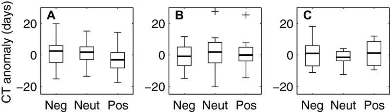
Fish phenology changed markedly during El Niño events, but the direction of changes depended on phenology group. For species that exhibited a decadal shift toward earlier phenology, El Niño (La Niña) was also associated with earlier (later) occurrence of larvae (Fig. 2A; Kruskal–Wallis, χ² = 7.5, df = 2,57, P < 0.05). This result suggested that fishes in this group reacted similarly to warming at the interannual scale associated with ENSO and the decadal scale. In contrast, species in the two other phenology groups experienced delays (advances) in spawning during El Niño (La Niña) (Fig. 2 B and C; species without a linear trend: F_2,63 = 6.3, P < 0.01; later species: F_2,24 = 5.3, P < 0.05). This response may reflect a late onset of upwelling and primary production during El Niño in the CCE (26).

Fig. 2.

Effects of El Niño-Southern Oscillation (A–C) and Pacific Decadal Oscillation (PDO; D–F) on species displaying earlier phenology (Left; n = 60), no long-term, linear change in phenology (Center; n = 66), and later phenology (Right; n = 27). In each box plot, the darkened line indicates the median; boxes show the interquartile range; whiskers indicate the expected extent of 99% of the data for a Gaussian distribution, and crosses show outliers. Two outliers fall outside the range displayed in A. Capital letters below boxes indicate means that differ significantly at P < 0.05 based on Tukey-Kramer multiple comparison tests. (A–C) El Niño, neutral (Neut), and La Niña conditions based on the Oceanic Niño Index. (D–F) Neg1, cold-phase PDO between 1951 and 1976; Pos, warm-phase PDO from 1977 to 1998; Neg2, cold-phase PDO during 1999–2002 and 2007–2008.

Attributing changes in phenology to the PDO is complicated by the fact that CalCOFI started during a negative cold PDO period that persisted through 1976 and was followed by a positive warm PDO phase continuing through 1998. Before 1998, the signal of anthropogenic climate change and warming related to the PDO were confounded. The return of negative PDO conditions in 1999 may potentially allow for clearer distinction between these influences on phenology (49). If the PDO was associated with changes in phenology, then the timing of larval occurrence during recent, negative PDO years should be similar to that observed during the earlier, negative PDO. To test for this effect, ANOVAs were performed comparing fish phenology during the first negative PDO phase (1951–1976), the second negative PDO phase (1999–2002 and 2007–2008), and the warm PDO phase (1977–1998; Fig. 2 D–F). These ANOVAs indicated that there were changes in phenology across these periods for both species with long-term delays and advances in phenology (earlier species: F_2,57 = 21.5, P < 0.001; later species: F_2,24 = 11.4, P < 0.001). No significant effects were observed for species without trends in phenology (F_2,63 = 0.1, P = 0.88). For advancing species, Tukey–Kramer multiple comparison tests revealed that these differences were due to changes in phenology between the recent, negative PDO and previous years (Fig. 2D). Phenology during the first, negative PDO differed from all subsequent periods among species with later phenology (Fig. 2F). In neither case were the first and second negative PDO periods similar to each other.

A similar analysis was conducted to evaluate whether fish phenology was influenced by negative, neutral, or positive NPGO conditions. ANOVAs testing this association were not significant for any phenology group (Fig. S3). This result again suggested that assemblage-wide changes in phenology may be more indicative of long-term trends than decadal climate variability.

Fig. S3.

Effects of the NPGO on the seasonal CT of fish species displaying earlier phenology (A; n = 60), no long-term, linear change in phenology (B; n = 66), and later phenology (C; n = 27). In each box plot, the darkened line indicates the median; boxes show the interquartile range; whiskers indicate the expected extent of 99% of the data for a Gaussian distribution, and crosses show outliers. Neg, NPGO index ≤−0.5; Neut, NPGO index between −0.5 and 0.5; Pos, NPGO index ≥0.5. ANOVA results for earlier species: F_2,57 = 1.6, P = 0.22; species without a linear trend: F_2,63 = 0.2, P = 0.81; later species: F_2,24 = 0.5, P = 0.61.

To further investigate which factors were responsible for changes in fish phenology, the effects of three locally measured oceanic variables (e.g., CalCOFI SST, CalCOFI zooplankton displacement volume, and the Bakun upwelling index) were examined. CT anomalies of these variables were calculated and regressed against time to assess decadal changes in seasonal patterns. Changes in SST CT indicated that ocean temperatures are now warming 25.9 d earlier than in the 1950s (Fig. 3A; Y = 33.7200 − 0.0170X, F = 11.0, df = 4, P < 0.05). Upwelling did not exhibit a significant trend in decadal phenology (Fig. S4A; F = 1.2, df = 4, P = 0.34), although peak upwelling during the 1980s and 2000s occurred slightly later than at the start of the time series. The CT of zooplankton volume was characterized by delayed phenology in the 1970s and early phenology in the 1980s (Fig. S4B), possibly reflecting changes related to the 1977 PDO shift (19). CT anomalies of zooplankton volume were close to zero in other decades, with no long-term trend (F = 1.0, df = 4, P = 0.30).

Fig. 3.

Responses of the phenology of larval fishes to changes in the central tendency (CT) of SST, zooplankton displacement volume, and the Bakun upwelling index at 33°N and 119°W. Units of all CT anomalies (CTa) are days. (A) Decadal changes in SST CT. SEs from bootstrap analysis are shown. (B–E) Multiple regression equations shown in Table S5. Variables included in a given regression, but not displayed on these bivariate plots, were held constant at a CT anomaly of zero.

Fig. S4.

Decadal changes in the CT of the Bakun upwelling index at 33°N and 119°W (A) and zooplankton volume from CalCOFI (B); 95% CIs from bootstrap analysis are shown. The white circle in A denotes the decadal CT of upwelling velocity within the CalCOFI area based on data from the QuikSCAT scatterometer.

Species in the earlier phenology group displayed significant, positive correlations with the CT of SST and zooplankton volume but were not influenced by upwelling (Fig. 3 and Table S5). Species whose phenology was delayed since the 1950s spawned later when the onset of upwelling also occurred later (Fig. 3D). In addition, this phenology group was inversely correlated with SST CT, such that fishes spawned earlier in years when seasonal temperatures remained cool for a longer time (Fig. 3B). CT anomalies for species with no long-term trends in phenology were not correlated with any oceanic variables (Table S5).

Table S5.

Stepwise multiple regressions between the three phenology groups and local oceanic conditions

Phenology group	Regression equation	df	AIC	F
Species with earlier phenology
Full dataset	Y = 0.0436 + 0.9120XSST + 0.2355XZoo − 0.3823XAR1	86	75.2	26.6***
Bias-corrected dataset	Y = -0.0250 + 1.2574XSST + 0.3690XZoo	87	116.6	10.2***
Species with no long-term, linear trend in phenology
Full dataset	Y = 0.0121	105	N/A	N/A
Bias-corrected dataset	Y = -0.0093 − 0.2898XAR1	104	152.7	9.3**
Species with later phenology
Full dataset	Y = 0.0518 − 0.4556XSST + 1.3534XUpw	40	33.8	7.5**
Bias-corrected dataset	Y = 0.0268 − 1.2713XSST + 1.8838XUpw	40	44.3	11.0***

In the regression equations, Y refers to CT anomalies of species in each phenology group, whereas X_SST, X_Zoo, and X_Upw are the CT of CalCOFI SST, CalCOFI mesozooplankton volume, and the Bakun upwelling index, respectively. X_AR1 is a first-order autoregressive term. Only the final regression model with the lowest AIC is shown. The bias-corrected dataset removes all data from May, September, and December, because missing data during these months in the 2000s could potentially affect results of this analysis. N/A, statistic could not be estimated because the null model provided the best fit to the data. Significance levels of regressions are indicated as follows: **P < 0.01; ***P < 0.001.

Next, this study investigated whether species that displayed phenological changes shared certain ecological traits. The characteristics examined were the six most common taxonomic orders, season of maximum larval abundance, the amplitude of a species’ seasonal cycle, trophic level, habitat of adult fishes, cross-shore distribution of larvae, biogeographic affinity (e.g., warm water, cool water, or widespread distribution), frequency of larval occurrence during surveys, and fishing status (Tables S1 and S2). The predominant modes of variability among these traits were characterized with PC analysis (PCA). The first two PCs constituted 45.5% of the variance in this dataset. An ordination of fishes with respect to these two PCs revealed three clusters of species with distinct traits (Fig. 4A). The first cluster was associated with positive loadings on PC1 and primarily negative loadings on PC2. Fishes in this group were mainly mesopelagic with an oceanic distribution (Fig. 4C). Myctophiformes and Stomiiformes were common in this cluster (Fig. 4B). The second cluster contained species with negative loadings on both PC1 and PC2. The distinguishing features of this cluster were that fishes used coastal, demersal habitats with cool water masses. Scorpaeniformes and Pleuroniformes were the two characteristic orders of fishes in this cluster. The third cluster indicated by positive loadings on PC2 was comprised of epipelagic fishes with a widespread, coastal-oceanic distribution, a high frequency of occurrence, and a large, seasonal amplitude (Fig. 4 C and D). Many fishes in this cluster belonged to the order Perciformes.

Fig. 4.

Principal components analysis performed on ecological traits (n = 51). (A) Species ordination. Marker size is proportional to changes in CT. Black (white) dots indicate species whose CT has a negative (positive) slope when regressed against year. (B) Eigenvectors of taxonomic orders. Stomi, Stomiiformes; Perci, Perciformes; Scorp, Scorpaeniformes; Mycto, Myctophiformes; Argen, Argentiniformes; Pleur, Pleuronectiformes. (C) Eigenvectors of adult fish habitat (epipelagic, mesopelagic, demersal), cross-shore distribution [coastal, coastal-oceanic (C-O), oceanic], and biogeographic affinity (cool water, warm water, widespread). (D) Eigenvectors of adult trophic level, fishing status, month of maximum larval abundance, frequency of occurrence, and amplitude of the seasonal cycle.

Both PC1 and PC2 were negatively correlated with changes in CT (r = −0.25 and −0.31, respectively). This relationship was significant at P < 0.05 for PC2, but marginally insignificant (P = 0.07) for PC1. Consequently, coastal-oceanic, epipelagic species in the third cluster mainly exhibited phenological advances, with a mean rate of change of −4.3 d/decade (Y = 28.2158 − 0.0142X₁, where Y = CT anomalies and X₁ = year, F = 3.9, df = 46, P = 0.05, Fig. 4A). Advancing phenology was also observed among 70% of oceanic, mesopelagic species in the first cluster. The rate of phenological change for this cluster was −3.0 d/decade (Y = 19.7065 − 0.0099X₁ – 0.2294X₂, where X₂ = first-order, autoregressive term, F = 11.4, df = 117, P < 0.001). Delayed phenology was detected most frequently among coastal, demersal fishes in the second cluster, although this group’s rate of phenological change was not statistically significant (F = 0.4, df = 93, P = 0.54). Based on a comparison between the current study and changes in the geographic distribution of the same fish species (50, 51), one additional ecological characteristic of the earlier phenology group was that they exhibited a higher probability of undergoing range shifts in response to changes in climatic and oceanic conditions (one-tailed binomial test: n = 16, P < 0.05).

Projections of 21st Century Changes in Phenology.

The Intergovernmental Panel on Climate Change (IPCC) Special Report on Emissions Scenarios (SRES) A1B scenario was used to forecast future changes in fish phenology. SRES A1B is a medium-range emissions scenario, where atmospheric CO₂ stabilizes at 720 ppm (52). Projections were based on the empirical relationship between local, oceanic variables and species with earlier or delayed phenology (Fig. 3 and Table S5). Changes in mean phenology between 2000–2009 and 2090–2099 were forecasted with 12 IPCC models run over an ensemble of 30 simulations. Models unanimously projected that SST would continue to warm earlier in the year through the 21st century. Predicted changes in SST CT between the 2000s and 2090s ranged between −1.5 and −18.0 d (mean = −10.1 d). In contrast, model outputs indicated high uncertainty in future changes in upwelling seasonality in the southern CCE, with 15 model runs predicting earlier upwelling and 11 predicting later upwelling. Mean change in upwelling CT between 2000–2009 and 2090–2099 was −4.4 d, with a range of −18.9 to 11.8 d. Projections for species with earlier phenology indicated that fishes would advance their phenology by −5.7 d on average relative to current conditions (Fig. 5; range, −0.1 to −10.4 d). Due to inconsistencies between models when forecasting changes in upwelling CT, projections suggested that species with later phenology may spawn anywhere between 21.6 d earlier to 22.1 d later compared with current conditions (Fig. 5B; mean = −1.7 d).

Fig. 5.

Projected changes in the phenology of larval fishes between 2000–2009 and 2090–2099 based on climate models from the IPCC Fourth Assessment Report. All projections are based on IPCC scenario A1B. Abbreviated IPCC names for each model are shown. (A) Species whose phenology became earlier during the 20th century. (B) Species whose phenology became later during the 20th century.

Discussion

Evaluation of Hypotheses.

This study indicated that the reproductive phenology of marine fishes showed varying responses to recent climate change that could be explained in part by the habitat used by each species. Despite the presence of strong natural climate variability in the CCE, long-term trends were detected in the phenology of 26 out of 43 fish species. Because trends in upwelling and zooplankton volume were not evident over this period, fishes with shifting phenology potentially could be subject to seasonal mismatches with lower trophic levels.

At the outset of this study, several hypotheses were proposed regarding phenological changes. The null hypothesis (H₀) stated that fish phenology would remain nearly constant through time. This outcome would be expected if a biological or environmental variable that exhibits little decadal variability were the primary influence on the timing of fish reproduction. For example, photoperiod is often cited as a process that affects the initiation of fish reproductive development (53) and displays little interannual variability. Although 22 fish phenophases (43%) showed no long-term trends, as is consistent with H₀, 29 phenophases (57%) displayed a decadal trend in phenology, suggesting a key role of climate. Furthermore, even species in the phenology group with no long-term trend exhibited interannual variations in larval occurrence associated with ENSO (Fig. 2B), indicating that their phenology was not as unwavering as suggested by H₀. Also, some species in this phenology group, such as S. sagax, displayed large interdecadal fluctuations in their phenology in absence of a long-term trend.

H_A1 proposed that earlier occurrence of larvae would be observed during periods with warm temperatures. Some support for H_A1 was provided by the positive correlation between SST CT and species with earlier phenology (Fig. 3C). Similar relationships between temperature and fish phenology were identified among ichthyoplankton in the North Sea and English Channel (11, 12). However, these studies considered a much smaller area (one to three sites), and their time series were not long enough to differentiate between the effects of climate change and climate variability.

Although the relationship identified between fish phenology and SST CT is correlative rather than mechanistic, several lines of evidence buttress this conclusion. First, temperature has a large physiological effect on fish reproduction due its influence on the production of hormones, vitellogenin, oocyte development, and egg survival (53). Because temperature accelerates gonadal maturation in poikilothermic fishes, changes in seasonal temperature measured in degree days has been used to forecast spawning time in diverse taxa (38–40). Second, species in each phenology group reacted similarly to decadal warming and changes in SST associated with ENSO indicating a consistent response of phenology to temperature across different time scales.

The effect of SST CT on larval phenology could reflect in part temperature-induced changes in the duration of the egg and larval stages among poikilotherms. Although a shortened duration of these life history stages under warmer temperatures could be partially responsible for phenological advances, it is unlikely that changes in stage duration alone could result in the observed rates of 3–12 d/decade of phenological change. The egg stage of many fishes only lasts 2–4 d at temperatures in the southern CCE (45). Also, larger, late-stage larvae that would be more affected by changes in stage duration were rare in CalCOFI samples (54). In addition to direct physiological effects, the influence of temperature on phenology may be mediated through other biological processes, such as seasonal migrations of fishes through regions with differing temperatures (12, 42) and the influence of temperature on seasonal prey availability (55).

Two hypotheses were proposed to explain delays in fish phenology. H_A2 suggested that fishes spawning in fall may exhibit delayed phenology if climate change leads to extended warm summer temperatures, whereas H_A3 asserted that delayed phenology would result from later onset of upwelling. This study provided scant support for H_A2, because the season of maximal larval abundance did not have a sizable effect on trends in fish phenology (Fig. 4D). Only two of the nine phenophases with delayed phenology were fall-spawning fishes. Although a long-term trend in upwelling seasonality was not observed (Fig. S4A), species with delayed phenology showed a positive correlation with upwelling CT (Fig. 3D), supporting H_A3. Upwelling could influence fish phenology through either offshore transport of larvae or augmentation of primary production. Among coastal, demersal fishes that were more likely to show delayed phenology (Fig. 4), it is imperative to minimize advection of larvae into unsuitable, offshore habitats. Because upwelling results in cross-shore transport, many coastal fishes spawn during winter when upwelling is minimal to increase retention (35). The phenology of these species may be positively correlated with the timing of upwelling to maintain their reproductive activity in synchrony with the winter lull in upwelling. For species whose larvae are most abundant in spring and summer, upwelling likely affects phenology through its impact of primary and secondary production, which increases prey availability.

H_A4 proposed that, in lieu of long-term trends, interannual-to-decadal variation in phenology associated with basin-scale climate cycles would be observed. Although ENSO was related to significant fluctuations in fish phenology, the PDO and NPGO did not have clear-cut effects (Fig. 2 and Fig. S3). This finding may initially seem surprising because the PDO and NPGO affect the abundance and geographic distribution of several species considered here (20, 44, 50, 51, 56). However, time series of CCE ocean temperature (a key factor controlling fish phenology) indicate that, although there have been PDO-like oscillations in the magnitude of this variable, there was also a concurrent, continuous shift in the phase of its seasonal cycle relative to a 1950s baseline (Fig. 3A) (21). This long-term phase shift may explain why the seasonality of larval fishes is less sensitive to the PDO. This result may be part of a more generalized pattern, because the PDO has a weak effect on the phenology of spring chinook salmon (O. tshawytscha) (29), a species whose abundance is strongly influenced by this climate cycle (57).

Rates of Current and Future Phenological Change.

In the southern CCE, fishes that spawn earlier during warm conditions advanced their phenology at a mean rate of 6.4 d/decade, whereas other species experienced mean delays of 5.1 d/decade. Assuming that temperature is a primary factor affecting fish phenology, the mean temperature sensitivity would be 24.6 d/°C for the earlier phenophases (range: 10.8–47.7 d/°C) and 19.6 d/°C for later phenophases (range: 11.5–27.7 d/°C), because this region warmed by 1.3 °C between 1949 and 2000 (58). When examining all phenology groups jointly using absolute values of phenological change, a mean of 4.7 ± 3.3 SD d/decade or 17.9 ± 12.8 SD d/°C was obtained. These rates were comparable to results from other studies of the phenology of marine and freshwater fishes and meroplankton (5, 7, 12, 40, 42, 59), but were faster than rates from many terrestrial ecosystems (1, 3, 4, 60). Although a sensitivity analysis suggested that this study may have limited power to detect shifts smaller than ∼3 d/decade (Table S3 and SI Text), it is unlikely that the phenological rates calculated here were biased fast because center of gravity metrics, such as CT, are usually conservative and change more slowly than the start date of phenological events (48, 61). Instead, the rapid changes observed in marine systems are more likely due to the smaller amplitude of seasonal temperature changes in marine habitats. This weak seasonal gradient implies that species need to undergo large phenological shifts to ensure that temperature-sensitive activities continue to occur at a constant temperature (8). Furthermore, the high fecundity and dispersal capacity of many fish species may allow them to adapt more rapidly than terrestrial organisms to changing conditions (6).

Another way in which these results differed from previous studies was that a lower percentage of phenophases responded to warming by occurring earlier. In the southern CCE, 39% of phenophases advanced their phenology. In contrast, >60% of species have responded to warming temperatures by advancing their phenology in many terrestrial (1, 3, 60) and aquatic systems (5, 11, 62). Studies of the changing geographic distribution of fishes in the southern CCE also showed that slightly less than half of the species were responsive to climate forcing (50, 51), suggesting that the large percentage of nonresponsive species may be characteristic of the southern CCE and possibly other EBCU ecosystems. This reduced phenological sensitivity to climate may be due to weak seasonality in the southern CCE, its high proportion of mesopelagic fishes that may be less exposed to variations in upper ocean climate (44, 56), or opposing trends in SST and upwelling seasonality.

In addition to long-term phenological advances, 18% of fish phenophases exhibited delayed phenology in the CCE. This percentage is higher than the equivalent percentage in many terrestrial habitats (1, 60) but is comparable to other subtropical, oceanic regions where delayed zooplankton phenology has been observed (63).

Future projections indicated that fishes in the earlier phenology group would advance their phenology at a mean rate of −0.6 d/decade (range: 0.01–1.2 d/decade), which is slower than their current rate of change. For the later phenology group, predictions were highly variable between model runs (Fig. 5B). Both the varying projections for delayed species and the slower rate of predicted change for advancing species may be related to the relatively low spatial resolution (≥1°) of most IPCC general circulation models (GCMs). This resolution limits the ability of models to represent fine-scale oceanographic dynamics associated with coastal upwelling (64, 65). As a result, most GCMs overestimate temperatures in EBCU systems (65). Overestimation of present day temperatures could potentially lead to an underestimation of future changes in temperature and phenology in these regions. Also, the coarse resolution of GCMs is likely related to the high variability between modeled upwelling rates observed here and in Wang et al. (64). Future predictions of fish phenology may be improved by either using regional climate models or the next generation of global GCMs, some of which will have resolutions as fine as 0.1° × 0.1°. Using the ensemble of IPCC-class models from the recent Coupled Model Intercomparison Project–Phase 5 (CMIP5) is unlikely to substantially affect these results because CMIP5 models have a similar spatial resolution to the models examined here and show a similar ensemble range of projected temperature changes over Western North America (52, 66). Even as higher-resolution GCMs become available, the accuracy of projections may be limited if there are thresholds beyond which fishes can no longer adapt to changing conditions by altering their phenology (67). Projections of changes in future fish phenology could also be improved by considering species range shifts, acclimation to changing oceanic conditions, and adaptation through natural selection.

Implications for Marine Ecology and Fisheries Management.

Only species in the earlier phenology group were influenced by variations in the seasonality of zooplankton volume. Even in this phenology group, the correlation between the CT of zooplankton and fishes only became evident after fluctuations in SST were taken into account. The diverging phenological trajectories of zooplankton and many fish species suggests that climate change may lead to an increased frequency of mismatches between trophic levels. During the early life history of fishes, mismatches can result in decreased foraging efficiency, slower growth, starvation, and lower survival (10, 34, 68). These impacts may eventually lead to poor recruitment, declines in abundance, and even local extinctions (33, 69), unless rapid evolution reverses phenological trends or density-dependent compensation occurs at a later life stage (70, 71). At times, mismatches between fishes and zooplankton can be transmitted up the food web to higher trophic levels (59).

Nevertheless, zooplankton displacement volume is a bulk measure of a myriad of species, including both predators and prey of larval fishes. Gelatinous organisms (e.g., cnidarians, ctenophores, pelagic tunicates) have a disproportionately large effect on CalCOFI measurements of zooplankton volume (72). Due to the low carbon content of gelatinous zooplankton, displacement volume may be a less than ideal indicator of prey availability for larval fishes. Monitoring of the phenology of individual zooplankton species or functional groups is needed to confirm whether mismatches between fishes and their prey are truly becoming more frequent.

Species that did not exhibit trends in phenology may also be vulnerable to global warming due to their reduced capacity to adapt to changing conditions. A lack of adaptive phenological change in some species has been associated with declining abundance (73). One additional indication of the vulnerability of species in the phenology group with no long-term trend is that their duration of peak larval abundance has contracted over time (74). A shorter spawning season increases the likelihood that in some years there will be little-to-no temporal overlap between larvae and environmental conditions conducive to their growth and survival. As a result, contracted spawning periods can be accompanied by greater recruitment variability (75).

These factors suggest that phenological plasticity may be a useful metric for predicting which species may benefit from or be impaired by climate change (73). Further evidence of the importance of phenological plasticity comes from the fact that fishes with earlier spawning were more likely to shift their geographic range in response to climatic variations (50, 51), suggesting a link between these two modes of adapting to climate change. Commonalities between species in each phenology group may prove useful for discerning how species yet to be studied will react to climate change. Characteristics that most strongly affected phenological trends were the habitats used by larval and adult fishes (Fig. 4). Taxonomy, relative abundance, and the amplitude of a species’ seasonal cycle influenced phenological trends to a lesser extent. Habitat not only influenced phenological trends, but is also a major factor affecting synchronous variations in fish abundance in the CCE (56). Epipelagic species using coastal-oceanic habitats were the group most likely to exhibit earlier spawning. Their phenological plasticity may reflect the fact that many of these species are batch spawners that can reproduce as frequently as once a week (76). These species also live in the upper water column where they are exposed to larger changes in climate. Last, epipelagic species typically have short life spans allowing for possible genetic adaptation to changing conditions. Other studies of climate change effects on fishes have indicated that pelagic species possess heightened climate sensitivity (77).

Current and future changes in fish phenology may necessitate that fishery managers implement precautionary and adaptive management approaches. Management activities that may be affected by changing phenology include (i) seasonal fishing closures designed to protect sensitive life stages or maintain sustainable escapement, (ii) stock assessment surveys timed to coincide with seasonal migrations or the occurrence of a key life history stage (e.g., daily egg production method surveys), and (iii) optimization of the release time of hatchery reared fish for stock enhancement (68). Monitoring long-term changes in phenology and periodically adjusting the timing of seasonal closures, surveys, and hatchery releases will be important for ensuring that management tactics remain effective. In cases where fish phenology is linked to cumulative, seasonal changes in temperature or other variables, it may be possible to develop short-term, operational forecasts to predict when a fishery should open or when a stock assessment survey should occur (78). In cases where climate change leads to increased phenological mismatches and resulting recruitment failure, the carrying capacity of an ecosystem may be reduced, necessitating changes to harvest guidelines. Longer rebuilding times of depleted stocks may also be needed if mismatches lead to prolonged periods of poor recruitment (79).

In conclusion, long-term changes in the spawning phenology of fishes were apparent in the CCE even though this region is strongly influenced by decadal-scale, natural climate variability. Among species whose phenology has become earlier since the 1950s, the mean rate of change was 6.4 d/decade. This rate was much faster than rates from many terrestrial ecosystems, but was comparable to phenological studies of other marine organisms, indicating that climate change may lead to a rapid reorganization of seasonal patterns in marine ichthyoplankton communities. Compared with historical changes, IPCC models appear to underestimate future projections of phenological change. In contrast to other ecosystems, both sustained advances and delays in phenology were observed in the CCE, reflecting the opposing influences of temperature and upwelling on phenology. Similar changes are likely to occur in other EBCU ecosystems if global warming alters the seasonal intensity of upwelling. Because zooplankton phenology did not change in synchrony with the seasonal larval abundance of many fishes, these species could be subject to increased mismatches with their prey.

Materials and Methods

Ichthyoplankton samples were collected by CalCOFI along six transects (lines 76.7–93.3), which extended offshore of California between San Diego (33.0°N) and north of Point Conception (35.1°N). During each cruise, 66 stations were typically surveyed with oblique tows of bongo or ring nets (Fig. S1). Kramer et al. described methods used to catch, preserve, and identify ichthyoplankton (41). Throughout this time series, two modifications were made to sampling methods. First, tow depth was increased from 140 to 210 m in 1969. This event was accompanied by a change from using a net with 550-μm silk mesh to a nylon net with a 505-μm mesh. Second, the 1.0-m ring net initially used to sample ichthyoplankton was replaced with a 0.71-m bongo net in 1977 (80). Although slightly more larvae >6.75 mm total length were caught with the bongo net, large larvae made up such a small fraction of total abundance that there was not a significant difference between the number of larvae captured by the two nets (54). The change in tow depth also had a minimal effect on abundance because most larvae resided at depths <125 m (56, 81). Data were averaged decadally to develop monthly time series.

Only taxa identified to species level were included in this analysis to avoid confounding changes in species composition with shifts in phenology (7). Cumulative rank occurrence of ichthyoplankton taxa sampled between 1951 and 1998 was used to select species for inclusion in this study. The 90th percentile of the cumulative rank occurrence curve included 43 species, which were examined here. Due to improvements over time in identifying larval fishes, some taxa were not consistently identified during the first two decades of CalCOFI. As a result, insufficient data were available to analyze three species during the 1950s (Argyropelecus sladeni, Lestidiops ringens, Oxyjulis californica) and an additional three species during both the 1950s and 1960s (Cyclothone signata, Danaphos oculatus, Melamphaes lugubris).

Some species exhibited peaks in larval abundance during both spring and fall. In such cases, three criteria were used to determine whether a species with several seasonal peaks in abundance should be classified as having multiple phenophases. First, peaks in abundance must be separated by ≥3 mo. Second, the amplitude of each peak must be >50% of the annual range of larval abundance. Third, the dip in abundance between peaks must encompass >35% of the annual range. Mean seasonal abundance from the full time series was used to evaluate these criteria.

CT was used as the main measure of phenology in this study because it accounted for data collected during all seasons, can be calculated from a time series with a monthly resolution, and is a conservative metric that is unlikely to overestimate the rate of phenological change (61). The CT of each phenophase was calculated with the following equation (7):

$$CT={\displaystyle \sum _{i=1}^{12}\left(m_i\times a_i\right)}/{\displaystyle \sum _{i=1}^{12}{a}_i},$$

where a_i was mean abundance of larvae in month m_i, such that i = 1, 2,…12 denoted January, February,…December. For species with two phenophases, each year was divided into two 6-mo periods (typically January–June and July–December) for which the CT was computed. For species whose abundance increased between December and January, the CT was calculated so that i = 1 referred to the month when the seasonal rise in abundance started. Phenological anomalies were calculated relative to the mean of the CTs from the six decades examined to ensure that each decade was weighted equally regardless of whether fish abundance was high or low. An anomaly of 1 indicated a 1-mo change in phenology. To convert monthly anomalies into daily values, they were multiplied by 30.44.

Two approaches were applied to examine assemblage-wide trends in phenology. First, a linear regression was performed in which decadal CT anomalies of all phenophases were regressed against year. Here and elsewhere phenophases were treated as replicates for examining assemblage-wide patterns. The slope of this regression was used to estimate the mean rate of change in days per decade. First-order, autoregressive (AR1) terms were incorporated into this regression and all other temporal analyses when AR1 terms were significant at P < 0.05 and the inclusion of AR1 minimized the Akaike information criterion (AIC). Second, PCA was used to reduce the dimensionality of the community composition data while further assessing changes within the assemblage’s first mode of variability. The CT of each phenophase was standardized by its mean and SD to give equal weight to all phenophases in the PCA (82). Species with missing data from the 1950s and 1960s were excluded from this analysis, so that the correlation matrix for the PCA would be complete.

Phenophases were classified into three groups based on correlations between CT anomalies and year. Phenophases with r ≤ −0.5 were categorized as exhibiting earlier phenology; correlations between −0.5 and 0.5 indicated no long-term, linear change; and phenophases with r ≥ 0.5 were classified as displaying later phenology. Note that |r| ≥ 0.5 does not correspond to a specific threshold of statistical significance, but is instead intended to provide a liberal indication of the direction of phenological change. As was done for the assemblage-wide mean, the slope of regressions between CT anomalies and year (plus an AR1 term, if statistically significant) were used to estimate rates of change for phenophases in each group. Monte Carlo simulation was used to determine the CIs for long-term changes in CT (SI Text and Tables S3 and S4). SI Text and Fig. S2 also include an evaluation of potential bias due to missing data from May, September, and December during the 2000s.

This study examined how three basin-scale climate oscillations, three local oceanic variables, and nine ecological characteristics affected the phenology of larval fishes. Details of each analysis are described in the SI Text. Climate indices (e.g., ENSO, PDO, NPGO) were partitioned into a set of three categorical variables for use in ANOVA. Data on each fish phenophase were aggregated into bins corresponding to the categorical phases of the climate indices. CT anomalies of phenophases were then calculated relative to each climate index phase. Lilliefors’ test, Bartlett’s test, and plots of residuals were used to ascertain whether the ANOVA assumptions of normality, homoscedasticity, and independence of residuals were met (82). If an ANOVA indicated a significant climate effect, Tukey–Kramer multiple comparison tests were used post hoc to determine which climate phases exhibited significant phenological differences. The CT of local oceanic variables (e.g., CalCOFI SST, CalCOFI zooplankton volume, Bakun upwelling index) was calculated on a decadal basis to identify long-term trends and fluctuations in the seasonality of these variables. The Bakun upwelling index overestimates offshore transport across the CalCOFI region due to a discontinuity in the atmospheric pressure gradient related to the presence of coastal mountains (83). However, because this index has been measured consistently over time, this bias seems unlikely to result in a spurious trend in phenology (SI Text). Forward stepwise, multiple regressions were performed to investigate the relationship between the CT anomalies of oceanic variables and the CT anomalies of fishes in each phenology group. Because several ecological characteristics of fishes were correlated, PCA was used to identify major modes of variability among the ecological characteristics. The first two PCs of the ecological traits were then compared with changes in fish CT with Pearson correlation tests. SI Text and Table S6 also describe additional tests investigating interactions between trends in phenology, shifts in the geographic range of species, and decadal changes in larval abundance.

Table S6.

Contingency table showing the interaction between decadal trends in phenology and larval abundance

Decadal trends in phenology	Decadal trends in mean abundance
	Increase	No change	Decrease	Total
Earlier	7 (7.84)	8 (8.24)	5 (3.92)	20
No change	11 (8.63)	8 (9.06)	3 (4.31)	22
Later	2 (3.53)	5 (3.71)	2 (1.76)	9
Total	20	21	10	51
	Test results: χ2 = 2.7; df = 4; P = 0.62

The number of fish phenophases observed in each category is shown above. Numbers in parentheses indicate expected values if phenophases were randomly assigned to each category. The χ² test of independence was performed using the N − 1 adjustment for small sample size (88).

Projections of 21st century changes in phenology were based on a multimodel dataset developed during phase 3 of the World Climate Research Program’s (WCRP’s) Coupled Model Intercomparison Project (CMIP3) (www-pcmdi.llnl.gov/ipcc/about_ipcc.php). Of the 25 models included in CMIP3, 12 were selected for examination due to their ability to replicate the spatial signature of the PDO with a correlation of r ≥ 0.7 (64). Data on SST and coastal upwelling derived from meridional wind speed were extracted from CMIP3 to serve as predictors of changes in fish phenology. Thirty simulations from the ensemble of 12 models contained SST data. Wind speed was available from 26 simulations. Monthly data from the SRES A1B scenario were examined during 2000–2099 and averaged over 30–35°N and 117–125°W. Projections of seasonal upwelling were unaffected by whether winds were extracted from the full study area or solely the area west of Point Conception, where upwelling is maximal off southern California (17). To calculate the volume of offshore Ekman transport (Q_x), wind stress (τ) was first computed with the formula: τ_y = ρ_air C_d v², where v is meridional wind speed at an atmospheric pressure of 100 kPA, ρ_air is the density of air, and C_d is the drag coefficient (1.2 × 10⁻³) (84). Q_x was calculated from the equation Q_x = τ_y × (ρf)⁻¹, where ρ is the density of seawater and f is the Coriolis parameter (85). A mean surface water density of 1,024.5 kg/m³ and an f of 7.83 × 10⁻⁵ s⁻¹ (based on a mean latitude of 32.5°N) were assumed for the CalCOFI region. Q_x was multiplied by 100 because the Bakun upwelling index examined Ekman transport over 100 m of coastline (83). CT anomalies of SST and upwelling were calculated decadally from CMIP3 data using the 2000s as a baseline for computing anomalies. The regressions between CT anomalies of local, oceanic variables, and species with earlier or delayed phenology (Fig. 3 and Table S5) were used to make projections of future phenological change. Because zooplankton volume is not included as a state variable in CMIP3 models, a CT anomaly of zero was assumed for this term in the regression for earlier species. Multimodel means of phenological change were calculated such that each model received equal weight regardless of the number of simulations run per model.

SI Text

Precision of Estimates of Phenological Change and Evaluation of Bias due to Gaps in Sampling.

A sensitivity analysis based on Monte Carlo simulation was conducted to quantify observation error related to noise from variations in larval abundance and the sparse, seasonal sampling resolution of CalCOFI. First, the seasonal distribution of a simulated larval species was modeled with a Gaussian curve where June 15 was initially the mean date of larval occurrence and there was a 1-mo SD. This standard deviation implied that 95% of larvae would be observed within ±2 mo of the mean. The Gaussian curve was multiplied by 10 to more realistically approximate larval abundance in the CalCOFI region. Variations in larval abundance that could affect the calculation of seasonal central tendency (CT) were stochastically generated from a coefficient of variation (CV) ranging between 0.05 and 0.60. Twelve CVs separated by 0.05 intervals were used. This range was selected based on the empirical CV of monthly larval abundance for representative species sampled by CalCOFI (e.g., Argentina sialis, Engraulis mordax, Lipolagus ochotensis, Scomber japonicus, Tetragonurus cuvieri). Next, shifts in phenology at rates of 0–12 d/decade were simulated over six decadal time steps. For each time step, the CT was calculated from monthly mean values extracted from the underlying continuous Gaussian distribution. This process was repeated 1,000 times for each CV and rate of phenological change. The 90% and 95% CIs of CT were calculated based on these simulated values to assess the precision of this estimate of phenological change.

For the largest CV considered, the 90% and 95% CIs of CT always fell within ±2.8–3.1 and ±3.3–3.6 d/decade, respectively, of the simulated change in phenology (Tables S3 and S4). The 90% CIs corresponded closely to the minimum rate of change observed among species categorized as displaying earlier or later phenology (i.e., −2.8 d/decade for earlier species; 3.0 d/decade for later species). This finding confirmed that, despite the coarse, seasonal sampling resolution of CalCOFI, this study was able to obtain reliable estimates of which species exhibited shifts in phenology.

A second potential source of error stemmed from the fact that no CalCOFI surveys were conducted in May, September, or December during the 2000s. These data gaps could skew estimates of CT from this decade and bias interdecadal trends. To evaluate this bias, I recalculated CT after removing these months from the entire time series so that all decades would have an identical monthly distribution of data. The first principal component of this new dataset accounted for 29.9% of variance and continued to show a progression toward earlier phenology (Fig. S2B). However, phenological advancement was no longer evident when examining the mean CT for all 43 species (Fig. S2D). For the three phenology groups, decadal trends in CT were extremely similar regardless of whether the missing months were included or excluded from the analysis, indicating resiliency to this potential source of bias (Fig. S2 E–J). In addition to being able to detect divergent trends obscured by the mean, this is another reason why this analysis principally focused on the three phenology groups when investigating long-term, ecological changes.

Measurements of CalCOFI SST and mesozooplankton displacement volume were also unavailable during May, September, and December in the 2000s. Again, these months were removed from the time series in its entirety, and CT was recalculated to detect potential biases resulting from gaps in sampling. Stepwise multiple regressions between oceanic variables and phenology groups produced broadly consistent results regardless of whether the full dataset or the bias corrected dataset was used (Table S5). As a result, Fig. 3 only presents results from the full time series.

Relationships Between Phenology, Climate, Oceanic Conditions, and Ecological Traits.

The effects of three basin-scale climate oscillations (e.g., ENSO, PDO, and NPGO) and three local environmental variables (e.g., SST, zooplankton volume, and coastal upwelling) on fish phenology were examined. ENSO events were characterized with the Oceanic Niño Index (ONI) produced by the National Centers for Environmental Prediction (www.cpc.ncep.noaa.gov/products/analysis_monitoring/ensostuff/ensoyears.shtml). This index was selected because it defines the onset and termination of El Niño and La Niña on a monthly basis. The PDO index was obtained from the Joint Institute for the Study of the Atmosphere and Ocean (57) (research.jisao.washington.edu/pdo/PDO.latest). The NPGO index was developed and made available by Emanuele Di Lorenzo at the Georgia Institute of Technology (30) (www.o3d.org/npgo/npgo.php). SST and mesozooplankton displacement volume were measured at CalCOFI stations where ichthyoplankton samples were collected. Gelatinous organisms with biovolumes >5 cm³ were excluded from measurements of zooplankton volume (41). Zooplankton volume from 1969 to 1977 was multiplied by a correction factor of 1.366 to account for changes in net type and tow depth (80). The monthly Bakun upwelling index from 33°N and 119°W was obtained from the Environmental Research Division at the Southwest Fisheries Science Center (83) (www.pfel.noaa.gov/products/PFEL/modeled/indices/upwelling/upwelling.html). This index estimates offshore Ekman volume transport based on atmospheric pressure fields. At 33° N and 119° W, the Bakun upwelling index overestimates offshore transport due to a discontinuity in the atmospheric pressure gradient related to the presence of coastal mountains (83). Nevertheless, this index is still correlated with upwelling measured with the QuikSCAT scatterometer at r = 0.6 (86). Also, the CT of QuikSCAT upwelling over the CalCOFI region during the 2000s fell within the 95% CI of the Bakun upwelling index CT from this decade (Fig. S4).

Each climate index was partitioned into three categorical variables for use in ANOVA. The ONI was divided into La Niña, El Niño, and neutral periods. PDO categories included (i) a negative PDO between 1951 and 1976; (ii) a positive PDO between 1977 and 1998; and (iii) a second, negative PDO in 1999–2002 and 2007–2008 (87). The years 2003–2006 were excluded because there were insufficient data to construct a monthly time series of larvae during this second positive PDO. Positive, neutral, and negative NPGO periods were defined on a monthly basis according to whether this index had a value ≥0.5, between 0.5 and −0.5, or ≤−0.5, respectively. These thresholds were selected so that there were an approximately equal number of months in each NPGO category. Data on each fish phenophase were aggregated into bins corresponding to different phases of the climate indices. CT anomalies of the fish phenophases were then calculated for each phase of the climate indices. Initially, crossed, two-way ANOVAs were performed using climate index and phenology group as independent variables. Because significant interactions were observed between most phenology groups and climate indices, separate one-way ANOVAs were performed to evaluate climate effects on each phenology group. Lilliefors’ test, Bartlett’s test, and plots of residuals were used to ascertain whether the assumptions of normality, homoscedasticity, and independence of residuals were met (82). Lilliefors’ test indicated that the assumption of normality was violated for the ANOVA examining ENSO effects on the earlier phenology group. As a result, a nonparametric Kruskall–Wallis test was performed in lieu of ANOVA. If an ANOVA or Kruskall–Wallis test revealed a significant climate effect, Tukey–Kramer multiple comparison tests were used post hoc to determine which climate phases exhibited significant phenological differences.

CalCOFI SST, CalCOFI zooplankton volume, and the Bakun upwelling index were selected as the local environmental variables to be examined due to known interannual-to-decadal variations in their seasonality (19, 21, 22, 25) and their potential to affect fish phenology through physiological and trophic pathways. The CT of these variables was calculated decadally for years between 1951 and 2008. Unlike upwelling and larval fish abundance, measurements of SST and zooplankton volume never approached zero during any month of the year. This pattern weakened the weighting of these variables by month when calculating the CT, resulting in a CT skewed toward the middle of the year. To increase the influence of monthly weights, the minimum monthly mean value (e.g., 13 °C for SST and 38 cm³/1,000 m³ of seawater strained for zooplankton volume) was subtracted from the decadally averaged time series before calculating the CT. After computing the CT of each variable, its SE was estimated with a bootstrap approach (82). Forward stepwise, multiple regressions were used to examine the relationship between the CT anomalies of environmental variables and the CT anomalies of fishes in each phenology group. A first-order, autoregressive (AR1) terms was also included as a variable in these regressions. The Akaike information criterion (AIC) was used to determine which variables resulted in the best regression fit.

Nine characteristics of species related to their phylogeny, ecology, and fishery status were evaluated to assess whether they affected rates of phenological change. These characteristics included taxonomic order, month of maximal larval abundance, trophic level, habitat use by adult fishes, cross-shore distribution, biogeographic affinity, fishing status, the log₁₀ transformed frequency of larval occurrence during CalCOFI surveys, and the log_e(x + 1) transformed amplitude of a species’ mean seasonal cycle. Tables S1 and S2 describes classification of fishes with respect to these characteristics. Taxonomic orders were only examined if data were available for at least five phenophases in that order. Initially, the mesopelagic category of habitats used by adult fishes was farther subdivided into vertically migrating and nonmigratory mesopelagic species. These classifications were later merged because no significant difference was observed between migratory and nonmigratory mesopelagic fishes in terms of phenological changes. Because several ecological traits were correlated, a PCA was performed to detect major modes of variability among ecological variables. Categorical variables (i.e., taxonomic order, adult fish habitat, cross-shore distribution, biogeographic affinity, and fishing status) were converted into dummy variables before PCA (82). Each variable was then standardized based on its mean and SD to ensure that all variables were given equal weight in the PCA (82). Correlations between the first two principal components of the ecological characteristics and changes in larval fish CT were assessed. The PCA revealed three groups of fishes with similar ecological characteristics (Fig. 4A). Phenological trends over time were examined for each of these groups.

This study also explored whether species that underwent shifts in phenology were more likely to change their geographic range in response to fluctuating climatic conditions. This analysis entailed a comparison between the results of this study and those of Hsieh et al., who investigated climate-related shifts in the distribution of 35 of the species examined here (Table S2) (50, 51). One-tailed binomial tests were used to evaluate whether there was a >50% probability that species in each phenology group exhibited a range shift.

Last, this study examined whether there was an interaction between decadal trends in phenology and changes in the abundance of larval fishes. Mean abundance of larvae was calculated on a decadal basis for each of the 51 phenophases of CalCOFI fishes. Each phenophase was then categorized as exhibiting an increasing decadal trend in abundance, no change, or a decreasing trend using the same classification that was applied to generate the three fish phenology groups. Namely, phenophases with correlations between mean decadal abundance and year that exceeded r ≥ 0.5 were classified as displaying an increasing trend in abundance; correlations of r ≤ −0.5 were indicative of a decreasing trend in abundance, and correlations with intermediate values were categorized as exhibiting no long-term, linear trend. A χ² test of independence was performed to determine whether fishes in any phenology group were more likely than would be expected by random chance to display a trend in abundance. The N − 1 correction described by Campbell (88) was used in the χ² test to account for small sample size. The results of this test were not significant (χ² = 2.7, df = 4, P = 0.62; Table S6), indicating that there was no interaction between phenology groups and the likelihood of fish species undergoing decadal declines or increases in abundance.

References

- 1.Parmesan C, Yohe G. A globally coherent fingerprint of climate change impacts across natural systems. Nature. 2003;421(6918):37–42. doi: 10.1038/nature01286. [DOI] [PubMed] [Google Scholar]
- 2.Root TL, et al. Fingerprints of global warming on wild animals and plants. Nature. 2003;421(6918):57–60. doi: 10.1038/nature01333. [DOI] [PubMed] [Google Scholar]
- 3.Menzel A, et al. European phenological response to climate change matches the warming pattern. Glob Change Biol. 2006;12(10):1969–1976. [Google Scholar]
- 4.Parmesan C. Influences of species, latitudes and methodologies on estimates of phenological response to global warming. Glob Change Biol. 2007;13(9):1860–1872. [Google Scholar]
- 5.Poloczanska ES, et al. Global imprint of climate change on marine life. Nature Clim Change. 2013;3:919–925. [Google Scholar]
- 6.Richardson AJ, Poloczanska ES. Ocean science. Under-resourced, under threat. Science. 2008;320(5881):1294–1295. doi: 10.1126/science.1156129. [DOI] [PubMed] [Google Scholar]
- 7.Edwards M, Richardson AJ. Impact of climate change on marine pelagic phenology and trophic mismatch. Nature. 2004;430(7002):881–884. doi: 10.1038/nature02808. [DOI] [PubMed] [Google Scholar]
- 8.Burrows MT, et al. The pace of shifting climate in marine and terrestrial ecosystems. Science. 2011;334(6056):652–655. doi: 10.1126/science.1210288. [DOI] [PubMed] [Google Scholar]
- 9.Cushing DH. Plankton production and year-class strength in fish populations: An update of the match/mismatch hypothesis. Adv Mar Biol. 1990;26:249–293. [Google Scholar]
- 10.Durant JM, Hjermann DO, Ottersen G, Stenseth NC. Climate and the match or mismatch between predator requirements and resource availability. Clim Res. 2007;33(3):271–283. [Google Scholar]
- 11. Greve W, Prinage S, Zidowitz H, Nast J, Reiners F (2005) On the phenology of North Sea ichthyoplankton. ICES J Mar Sci 62(7):1216–1223.
- 12.Genner MJ, et al. Temperature-driven phenological changes within a marine larval fish assemblage. J Plankton Res. 2010;32(5):699–708. [Google Scholar]
- 13.Huyer A, Sobey JC, Smith RL. The spring transition in currents over the Oregon continental shelf. J Geophys Res. 1979;84(C11):6995–7011. [Google Scholar]
- 14.Lynn RJ, Bograd SJ, Chereskin TK, Huyer A. Seasonal renewal of the California Current: The spring transition off California. J Geophys Res. 2003;108(C8):1–11. [Google Scholar]
- 15.Snyder MA, Sloan LC, Diffenbaugh NS, Bell JL. Future climate change and upwelling in the California Current. Geophys Res Lett. 2003;30(15):1–4. [Google Scholar]
- 16.Henson SA, Thomas AC. Interannual variability in timing of bloom initiation in the California Current System. J Geophys Res. 2007;112(C08007):1–12. [Google Scholar]
- 17.Mantyla AW, Bograd SJ, Venrick EL. Patterns and controls of chlorophyll-a and primary productivity cycles in the Southern California Bight. J Mar Syst. 2008;73(1-2):48–60. [Google Scholar]
- 18.Kim H-J, Miller AJ, McGowan J, Carter ML. Coastal phytoplankton blooms in the Southern California Bight. Prog Oceanogr. 2009;82(2):137–147. [Google Scholar]
- 19.McGowan JA, Bograd SJ, Lynn RJ, Miller AJ. The biological response to the 1977 regime shift in the California Current. Deep Sea Res Part II Top Stud Oceanogr. 2003;50(14-16):2567–2582. [Google Scholar]
- 20.Moser HG, et al. Distributional Atlas of Fish Larvae and Eggs in the Southern California Bight Region: 1951-1998. California Cooperative Oceanic Fisheries Investigations Atlas 34. National Marine Fisheries Service, Southwest Fisheries Science Center; La Jolla, CA: 2001. [Google Scholar]
- 21.Mendelssohn R, Schwing FB, Bograd SJ. Nonstationary seasonality of upper ocean temperature in the California Current. J Geophys Res. 2004;109(C10015):1–16. [Google Scholar]
- 22.Venegas RM, et al. Satellite-derived variability in chlorophyll, wind stress, sea surface height, and temperature in the northern California Current System. J Geophys Res. 2008;113(C03015):1–18. [Google Scholar]
- 23.Schwing FB, Mendelssohn R. Increased coastal upwelling in the California Current System. J Geophys Res. 1997;102(C2):3421–3438. [Google Scholar]
- 24.Diffenbaugh NS, Snyder MA, Sloan LC. Could CO(2)-induced land-cover feedbacks alter near-shore upwelling regimes? Proc Natl Acad Sci USA. 2004;101(1):27–32. doi: 10.1073/pnas.0305746101. [DOI] [PMC free article] [PubMed] [Google Scholar]
- 25.Bograd SJ, et al. Phenology of coastal upwelling in the California Current. Geophys Res Lett. 2009;36(L01602):1–5. [Google Scholar]
- 26.Yoo S, Batchelder HP, Peterson WT, Sydeman WJ. Seasonal, interannual and event scale variation in North Pacific ecosystems. Prog Oceanogr. 2008;77(2-3):155–181. [Google Scholar]
- 27.Sasaoka K, Chiba S, Saino T. Climatic forcing and phytoplankton phenology over the subarctic North Pacific from 1998 to 2006, as observed from ocean color data. Geophys Res Lett. 2011;38(L15609):1–6. [Google Scholar]
- 28.Brodeur RD, Gadomski DM, Pearcy WG, Batchelder HP, Miller CB. Abundance and distribution of ichthyoplankton in the upwelling zone off Oregon during anomalous El Niño conditions. Estuar Coast Shelf Sci. 1985;21(3):365–378. [Google Scholar]
- 29.Keefer ML, Peery CA, Caudill CC. Migration timing of Columbia River spring chinook salmon: Effects of temperature, river discharge, and ocean environment. Trans Am Fish Soc. 2008;137(4):1120–1133. [Google Scholar]
- 30.Di Lorenzo E, et al. North Pacific Gyre Oscillation links ocean climate and ecosystem change. Geophys Res Lett. 2008;35(L08607):1–6. [Google Scholar]
- 31.Anderson JT. A review of size dependent survival during pre-recruit stages of fishes in relation to recruitment. J Northwest Atl Fish Sci. 1988;8:55–66. [Google Scholar]
- 32.Houde ED. Emerging from Hjort’s shadow. J Northwest Atl Fish Sci. 2008;41:53–70. [Google Scholar]
- 33.Beaugrand G, Brander KM, Alistair Lindley J, Souissi S, Reid PC. Plankton effect on cod recruitment in the North Sea. Nature. 2003;426(6967):661–664. doi: 10.1038/nature02164. [DOI] [PubMed] [Google Scholar]
- 34.Platt T, Fuentes-Yaco C, Frank KT. Marine ecology: Spring algal bloom and larval fish survival. Nature. 2003;423(6938):398–399. doi: 10.1038/423398b. [DOI] [PubMed] [Google Scholar]
- 35.Parrish RH, Nelson CS, Bakun A. Transport mechanisms and reproductive success of fishes in the California Current. Biol Oceanogr. 1981;1(2):175–203. [Google Scholar]
- 36.Mackas DL, Batten S, Trudel M. Effects on zooplankton of a warmer ocean: Recent evidence from the Northeast Pacific. Prog Oceanogr. 2007;75(2):223–252. [Google Scholar]
- 37.Koeller P, et al. Basin-scale coherence in phenology of shrimps and phytoplankton in the North Atlantic Ocean. Science. 2009;324(5928):791–793. doi: 10.1126/science.1170987. [DOI] [PubMed] [Google Scholar]
- 38.Ware DM, Tanasichuk RW. Biological basis of maturation and spawning waves in Pacific herring (Clupea harengus pallasi) Can J Fish Aquat Sci. 1989;46(10):1776–1784. [Google Scholar]
- 39.Lange U, Greve W. Does temperature influence the spawning time, recruitment and distribution of flatfish via its influence on the rate of gonadal maturation? Dtsch Hydrogr Z. 1997;49(2-3):251–263. [Google Scholar]
- 40.Gillet C, Quétin P. Effect of temperature change on the reproductive cycle of roach in Lake Geneva from 1983 to 2001. J Fish Biol. 2006;69(2):518–534. [Google Scholar]
- 41.Kramer D, Kalin MJ, Stevens EG, Thrailkill JR, Zweifel JR. Collecting and Processing Data on Fish Eggs and Larvae in the California Current Region. NOAA Technical Report NMFS CIRC-370. National Marine Fisheries Service; Seattle: 1972. [Google Scholar]
- 42.Jansen T, Gislason H. Temperature affects the timing of spawning and migration of North Sea mackerel. Cont Shelf Res. 2011;31(1):64–72. [Google Scholar]
- 43.Methot RD. Seasonal variation in survival of larval northern anchovy, Engraulis mordax, estimated from the age distribution of juveniles. Fish Bull. 1983;81(4):741–750. [Google Scholar]
- 44.Koslow JA, Goericke R, Lara-Lopez A, Watson W. Impact of declining intermediate-water oxygen on deepwater fishes in the California Current. Mar Ecol Prog Ser. 2011;436:207–218. [Google Scholar]
- 45.Zwiefel JR, Lasker R. Prehatch and posthatch growth of fishes—A general model. Fish Bull. 1976;74(3):609–621. [Google Scholar]
- 46.Moser HG. The Early Stages of Fishes in the California Current Region. California Cooperative Oceanic Fisheries Investigations Atlas 33. Allen Press; Lawrence, KS: 1996. [Google Scholar]
- 47.Love MS, Yoklavich M, Thorsteinson L. The Rockfishes of the Northeast Pacific. Univ of California Press; Los Angeles: 2002. [Google Scholar]
- 48.Miller-Rushing AJ, Inouye DW, Primack RB. How well do first flowering dates measure plant responses to climate change? The effects of population size and sampling frequency. J Ecol. 2008;96(6):1289–1296. [Google Scholar]
- 49.Stewart IT, Cayan DR, Dettinger MD. Changes toward earlier streamflow timing across Western North America. J Clim. 2005;18(8):1136–1155. [Google Scholar]
- 50.Hsieh CH, Reiss CS, Hewitt RP, Sugihara G. Spatial analysis shows that fishing enhances the climatic sensitivity of marine fishes. Can J Fish Aquat Sci. 2008;65(5):947–961. [Google Scholar]
- 51.Hsieh CH, Kim HJ, Watson W, Di Lorenzo E, Sugihara G. Climate-driven changes in abundance and distribution of larvae of oceanic fishes in the southern California region. Glob Change Biol. 2009;15(9):2137–2152. [Google Scholar]
- 52.IPCC . In: Climate Change 2007: The Physical Science Basis. Contribution of Working Group I to the Fourth Assessment Report of the Intergovernmental Panel on Climate Change. Solomon S, et al., editors. Cambridge Univ Press; Cambridge, UK: 2007. [Google Scholar]
- 53.Pankhurst NW, Munday PL. Effects of climate change on fish reproduction and early life history stages. Mar Freshw Res. 2011;62(9):1015–1026. [Google Scholar]
- 54.Hewitt R. Distributional Atlas of Fish Larvae in the California Current Region: Northern Anchovy, Engraulis mordax (Girard), 1966-1979. California Cooperative Oceanic Fisheries Investigations Atlas 28. National Marine Fisheries Service, Southwest Fisheries Science Center; La Jolla, CA: 1980. [Google Scholar]
- 55.Carscadden J, Nakashima BS, Frank KT. Effects of fish length and temperature on the timing of peak spawning in capelin (Mallotus villosus) Can J Fish Aquat Sci. 1997;54(4):781–787. [Google Scholar]
- 56.Koslow JA, Goericke R, Watson W. Fish assemblages in the Southern California Current: Relationships with climate, 1951-2008. Fish Oceanogr. 2013;22(3):207–219. [Google Scholar]
- 57.Mantua NJ, Hare SR, Zhang Y, Wallace JM, Francis RC. A Pacific decadal climate oscillation with impacts on salmon production. Bull Am Meteorol Soc. 1997;78(6):1069–1079. [Google Scholar]
- 58.Di Lorenzo E, Miller AJ, Schneider N, McWilliams JC. The warming of the California Current System: Dynamics and ecosystem implications. J Phys Oceanogr. 2005;35(3):336–362. [Google Scholar]
- 59.Frederiksen M, Elston DA, Edwards M, Mann AD, Wanless S. Mechanisms of long-term decline in size of lesser sandeels in the North Sea explored using a growth and phenology model. Mar Ecol Prog Ser. 2011;432:137–147. [Google Scholar]
- 60.Miller-Rushing AJ, Primack RB. Global warming and flowering times in Thoreau’s Concord: A community perspective. Ecology. 2008;89(2):332–341. doi: 10.1890/07-0068.1. [DOI] [PubMed] [Google Scholar]
- 61.Ji R, Edwards M, Mackas DL, Runge JA, Thomas AC. Marine plankton phenology and life history in a changing climate: Current research and future directions. J Plankton Res. 2010;32(10):1355–1368. doi: 10.1093/plankt/fbq062. [DOI] [PMC free article] [PubMed] [Google Scholar]
- 62.Thackeray SJ, et al. Trophic level asynchrony in rates of phenological change for marine, freshwater and terrestrial environments. Glob Change Biol. 2010;16(12):3304–3313. [Google Scholar]
- 63.Mackas DL, et al. Changing zooplankton seasonality in a changing ocean: Comparing time series of zooplankton phenology. Prog Oceanogr. 2012;97-100:31–62. [Google Scholar]
- 64.Wang M, Overland JE, Bond NA. Climate projections for selected large marine ecosystems. J Mar Syst. 2010;79(3-4):258–266. [Google Scholar]
- 65.Stock CA, et al. On the use of IPCC-class models to assess the impact of climate on Living Marine Resources. Prog Oceanogr. 2011;88(1-4):1–27. [Google Scholar]
- 66.IPCC . In: Climate Change 2013: The Physical Science Basis. Contribution of Working Group I to the Fifth Assessment Report of the Intergovernmental Panel on Climate Change. Stocker TF, et al., editors. Cambridge Univ Press; Cambridge, UK: 2013. [Google Scholar]
- 67.Neuheimer AB, Thresher RE, Lyle JM, Semmens JM. Tolerance limit for fish growth exceeded by warming waters. Nature Clim Change. 2011;1:110–113. [Google Scholar]
- 68.Chittenden CM, et al. Recent salmon declines: A result of lost feeding opportunities due to bad timing? PLoS ONE. 2010;5(8):e12423. doi: 10.1371/journal.pone.0012423. [DOI] [PMC free article] [PubMed] [Google Scholar]
- 69.Burkle LA, Marlin JC, Knight TM. Plant-pollinator interactions over 120 years: Loss of species, co-occurrence, and function. Science. 2013;339(6127):1611–1615. doi: 10.1126/science.1232728. [DOI] [PubMed] [Google Scholar]
- 70.Anderson JJ, Gurarie E, Bracis C, Burke BJ, Laidre KL. Modeling climate change impacts on phenology and population dynamics of migratory marine species. Ecol Modell. 2013;264:83–97. [Google Scholar]
- 71.Reed TE, Grøtan V, Jenouvrier S, Sæther BE, Visser ME. Population growth in a wild bird is buffered against phenological mismatch. Science. 2013;340(6131):488–491. doi: 10.1126/science.1232870. [DOI] [PubMed] [Google Scholar]
- 72.Lavaniegos BE, Ohman MD. Coherence of long-term variations of zooplankton in two sectors of the California Current System. Prog Oceanogr. 2007;75(1):42–69. [Google Scholar]
- 73.Cleland EE, et al. Phenological tracking enables positive species responses to climate change. Ecology. 2012;93(8):1765–1771. doi: 10.1890/11-1912.1. [DOI] [PubMed] [Google Scholar]
- 74.Asch RG. 2013. Interannual-to-decadal changes in phytoplankton phenology, fish spawning habitat, and larval fish phenology. PhD dissertation (Univ of California, San Diego)
- 75.Mertz G, Myers RA. Match/mismatch predictions of spawning duration versus recruitment variability. Fish Oceanogr. 1994;3(4):236–245. [Google Scholar]
- 76.Hunter JR, Goldberg SR. Spawning incidence and batch fecundity in northern anchovy, Engraulis mordax. Fish Bull. 1980;77(3):641–652. [Google Scholar]
- 77.Cheung WWL, et al. Projecting global marine biodiversity impacts under climate change scenarios. Fish Fish. 2009;10(3):235–251. [Google Scholar]
- 78.Greve W, Reiners F, Nast J, Hoffman S. Helgoland Roads meso- and macrozooplankton time-series 1974 to 2004: Lessons from 30 years of single spot, high frequency sampling at the only off-shore island of the North Sea. Helgol Mar Res. 2004;58(4):274–288. [Google Scholar]
- 79.Holt CA, Punt AE. Incorporating climate information into rebuilding plans for overfished groundfish species of the U.S. west coast. Fish Res. 2009;100(1):57–67. [Google Scholar]
- 80.Ohman MD, Smith PE. A comparison of zooplankton sampling methods in the CalCOFI time series. Calif Coop Ocean Fish Invest Rep. 1995;36:153–158. [Google Scholar]
- 81.Ahlstrom EH. Vertical distribution of pelagic fish eggs and larvae off California and Baja California. Fish Bull. 1959;60:107–146. [Google Scholar]
- 82.Quinn GP, Keough MJ. Experimental Design and Data Analysis for Biologists. Cambridge Univ Press; Cambridge, UK: 2002. [Google Scholar]
- 83.Bakun A. Coastal Upwelling Indices, West Coast of North America, 1946-71. NOAA Technical Report, NMFS SSRF-671. National Marine Fisheries Service; Seattle: 1973. [Google Scholar]
- 84.Trenberth KE, Large WG, Olson JG. The effective drag coefficient for evaluating wind stress over the oceans. J Clim. 1989;2(12):1507–1516. [Google Scholar]
- 85.Pond S, Pickard GL. Introductory Dynamic Oceanography. 2nd Ed Butterworth Heinemann; Oxford, UK: 1995. [Google Scholar]
- 86.Pérez-Brunius P, López M, Parés-Sierra A, Pineda J. Comparison of upwelling indices off Baja California derived from three different wind data sources. Calif Coop Ocean Fish Invest Rep. 2007;48:204–214. [Google Scholar]
- 87.Peterson WT. Copepod species richness as an indicator of long-term changes in the coastal ecosystem of the northern California Current. Calif Coop Ocean Fish Invest Rep. 2009;50:73–81. [Google Scholar]
- 88.Campbell I. Chi-squared and Fisher-Irwin tests of two-by-two tables with small sample recommendations. Stat Med. 2007;26:3661–3675. doi: 10.1002/sim.2832. [DOI] [PubMed] [Google Scholar]
- 89.Hsieh C-H, et al. A comparison of long-term trends and variability in populations of larvae of exploited and unexploited fishes in the Southern California region: A community approach. Prog Oceanogr. 2005;67:160–185. [Google Scholar]
- 90.Hsieh C-H, et al. Fishing elevates variability in the abundance of exploited species. Nature. 2006;443:859–862. doi: 10.1038/nature05232. [DOI] [PubMed] [Google Scholar]
- 91.Field JC, Francis RC, Aydin K. Top-down modeling and bottom-up dynamics: Linking a fisheries-based ecosystem model with climate hypotheses in the Northern California Current. Prog Oceanogr. 2006;68:238–270. [Google Scholar]