

Abstract.
Image heterogeneity metrics such as textural features are an active area of research for evaluating clinical outcomes with positron emission tomography (PET) imaging and other modalities. However, the effects of stochastic image acquisition noise on these metrics are poorly understood. We performed a simulation study by generating 50 statistically independent PET images of the NEMA IQ phantom with realistic noise and resolution properties. Heterogeneity metrics based on gray-level intensity histograms, co-occurrence matrices, neighborhood difference matrices, and zone size matrices were evaluated within regions of interest surrounding the lesions. The impact of stochastic variability was evaluated with percent difference from the mean of the 50 realizations, coefficient of variation and estimated sample size for clinical trials. Additionally, sensitivity studies were performed to simulate the effects of patient size and image reconstruction method on the quantitative performance of these metrics. Complex trends in variability were revealed as a function of textural feature, lesion size, patient size, and reconstruction parameters. In conclusion, the sensitivity of PET textural features to normal stochastic image variation and imaging parameters can be large and is feature-dependent. Standards are needed to ensure that prospective studies that incorporate textural features are properly designed to measure true effects that may impact clinical outcomes.
Keywords: quantitative, positron emission tomography, heterogeneity, textural features, simulation, standardization
1. Introduction
Quantification of image heterogeneity is a broad application associated with many fields, such as satellite imaging, facial recognition, and more recently, medical imaging. Medical image heterogeneity quantification may be relevant to descriptions of tumor phenotype, image segmentation, and outcome assessment. The developing field of radiomics focuses on large scale analysis of image metrics to build models correlating to clinical parameters or genomic signatures.1,2
The recent focus on quantitative positron emission tomography/computed tomography (PET/CT) is evident from initiatives from American Association of Physicists in Medicine (AAPM), Radiological Society of North America (RSNA), National Institutes of Health/National Cancer Institute (NIH/NCI), American College of Radiology Imaging Network (ACRIN), European Organization of Research and Treatment of Cancer (EORTC), and other groups.3 The goal of quantitative PET is to determine the relationship between an imaging metric and its natural variability due to technical, physical and biological processes unrelated to the clinical investigation, such as quality of dose administration, image reconstruction and duration of tracer uptake. Improving quantitative aspects of imaging studies may increase statistical power, reduce required patient accruals and diminish the duration and expense of clinical trials. There is a need to apply the lessons of quantitative imaging in a prospective manner as new imaging applications are developed.4,5
Considerable interest has been raised in the application of the so-called textural feature metrics, such as intensity histogram features, co-occurrence matrices,6 neighborhood difference matrices,7 and zone size matrices,8 to PET/CT imaging for clinical applications. Textural features have been correlated to clinical data such as survival, clinical response and prognostic pathological features in cervical, head and neck, lung, esophageal, rectal, and breast cancers.9–16
Despite the increased use of these metrics for PET imaging, relatively little is known about the impact of fundamental data acquisition and image reconstruction parameters on metric variability. The few studies to date have appropriately focused on test-retest or sensitivity studies in patient data.17–22 However, it is evident that increased understanding of the quantitative aspects of image heterogeneity metrics may improve the quality of clinical trials that incorporate their use.
The purpose of this study is to evaluate the quantitative variability caused by stochastic effects in conjunction with acquisition and image reconstruction parameters on PET/CT textural analysis metrics. This is achieved through the use of realistic phantom simulations in the ground truth setting. Variable object sizes with known activity were investigated, as well as sensitivity studies on the effects of patient size and image reconstruction on the variability of these metrics. Finally, representative statistical power studies are investigated to demonstrate implications for the use of these metrics in clinical trials. These results are intended to inform the design of prospective clinical trials using PET/CT image heterogeneity metrics as well as to motivate standardization and harmonization in their implementation.
2. Methods
2.1. Image Simulation
The determination of the variability of PET image values required the generation of many independent sets of projection data with realistic noise and resolution properties. To this end, the ASIM simulation tool was used to create noise-free attenuated sinograms from an analytical ground truth activity map.23,24 NEMA image quality-type phantoms with spherical objects of 10, 13, 17, 22, 28, and 37 mm diameters were simulated.25
The detector geometry was approximately that of a General Electric D690 PET/CT scanner. A radially varying kernel was convolved with the projection data to simulate cross talk between nearby detectors. A measured normalization array was used to impose physically realistic sensitivity variations on the data. A scatter estimate was obtained by blurring the projection data in both the radial and azimuthal directions. An estimate of random coincidences was included as a uniform sinogram. Scattered, random and prompt counts were scaled to match estimated count levels from a five minute acquisition of a physical NEMA IQ phantom. Poisson noise was then added to these scaled sinograms based on the acquisition duration.
The sinograms were reconstructed with a fully three-dimensional ordered subsets expectation maximization (OSEM) algorithm.26 Correction for physical effects such as scattered and random coincidences, attenuation, interdetector blur, and sensitivity were all applied as in-loop corrections. The default reconstruction was with two iterations and 28 subsets, and a Gaussian postfilter of 5-mm transaxially and 4.6-mm axially was applied. The reconstructed voxel size was . Fifty independent and identically distributed image realizations were simulated. The point spread function was included as an in-loop effect in the reconstructions. The ground truth activity map for the reference case along with three realizations incorporating realistic stochastic noise is depicted in Fig. 1.
Fig. 1.
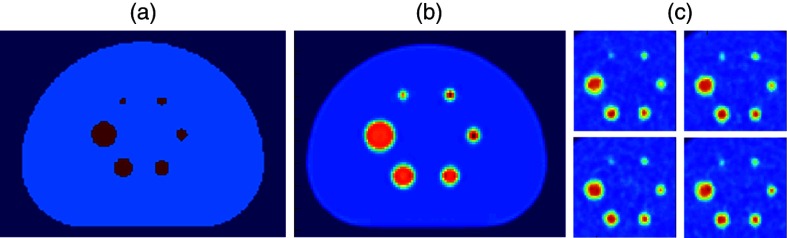
Fifty independent positron emission tomography (PET) images were simulated from a theoretical activity map derived from the NEMA image quality phantom with realistic physical constraints: (a) theoretical activity map, (b) noise free realization, and (c) 50 independent realizations.
2.2. Image Analysis
Regions of interest were defined on the theoretical activity map to define the ground truth location of the lesions and subsequently applied to each independent realization. Whole voxels whose centers were inside the radius of the lesion were included in the regions of interest. The five largest lesions were analyzed; the 10-mm lesions were not analyzed due to insufficient voxels. An 8-bit discretization was applied to image intensities for analysis. The investigated histogram and textural feature metrics are summarized in Table 1.
Table 1.
Textural features under investigation.
| Category | Feature |
|---|---|
| Based on intensity histogram (GLIH) | Standard deviation (SD) |
| Skewness (SKEW) | |
| Kurtosis (KURT) | |
| Energy (ENGY) | |
| Entropy (ENTR) | |
| Based on gray level neighborhood matrix (GLND)7,27 | Coarseness (COAR) |
| Contrast (CONT) | |
| Busyness (BUSY) | |
| Complexity (CPLX) | |
| Strength (STRG) | |
| Based on gray level co-occurrence matrix (GLCO)6,28 | Autocorrelation (AUTOC) |
| Contrast (CONTR) | |
| Correlation (CORR) | |
| Cluster prominence (CPROM) | |
| Dissimilarity (DISSI) | |
| Energy (ENERG) | |
| Entropy (ENTRO) | |
| Maximum probability (MAXPR) | |
| Sum of squares: variance (SOSVH) | |
| Sum average (SAVGH) | |
| Sum variance (SVARH) | |
| Sum entropy (SENTH) | |
| Difference variance (DVARH) | |
| Difference entropy (DENTH) | |
| Based on gray-level zone size matrix (GLZS)8 | Short zones emphasis (SZE) |
| Large zones emphasis (LZE) | |
| Low gray-level zones emphasis (LGZE) | |
| High gray-level zones emphasis (HGZE) | |
| Short zones low gray-level emphasis (SZLGE) | |
| Short zones high gray-level emphasis (SZHGE) | |
| Large zones low gray-level emphasis (LZLGE) | |
| Large zones high gray-level emphasis (LZHGE) | |
| Gray-level nonuniformity (GLNU) | |
| Zone size nonuniformity (ZSNU) | |
| Zone percentage (ZP) |
2.2.1. Intensity histogram features
The parameters derived from the intensity histogram of intratumoral PET voxels included standard deviation (SD), skewness (SKEW), kurtosis (KURT), energy (ENGY), and entropy (ENTR) with each characterizing the histogram from the aspect of dispersion, symmetry, peakedness, uniformity, and randomness, respectively. Also known as first-order or global texture measures, these parameters estimate properties of voxel values without correlating spatial information.
2.2.2. Gray level co-occurrence matrix-based features
In contrast to histogram-based features, texture parameters described by the gray-level co-occurrence method capture image properties pertaining to second-order statistics which accentuate the interaction and relationship between voxel values. This method examines pairwise voxel interaction of the image being investigated in terms of the gray-level co-occurrence matrix (GLCO). The GLCO has previously been described by Haralick et al.6,28 Briefly, it is created by recording the joint probability of frequency of gray-level values relative to another gray-level value appearing in a specified linear displacement. The texture features based on the GLCO used in the current analysis are presented in Table 1, including correlation (CORR), entropy (ENTR), and dissimilarity (DISSI). Correlation, for example, measures the linearity in the image, while entropy measures the amount of randomness of gray-level distribution in the image. The present implementation of this texture method considered a voxel displacement of 1 and each texture parameter was averaged along the 13 different angular directions.
2.2.3. Gray level neighborhood difference matrix-based features
The neighborhood gray level difference method exploits properties of visual perception by describing images in terms of the gray-level difference between image voxels and their neighboring voxels, which is encoded in the gray-level neighborhood difference matrix (GLND).7,27 The five attributes of texture deduced from GLND consist of coarseness (COAR), contrast (CONT), busyness (BUSY), complexity (CPLX), and strength (STRG), as listed in Table 1. Large values of coarseness indicate that gray-level differences are small in the image, whereas high contrast means the gray-level difference between neighboring regions is large. Busyness measures the rapidness of gray-level change from a voxel to its neighbors. A texture is considered strong when its constituent primitives (basic patterns) are easily defined and complex when there are many primitives of different intensities. In the present study, a neighborhood size of was considered. Neighborhood difference metrics could not be calculated for the 13 mm lesions as there were insufficient voxels to form a contiguous matrix.
2.2.4. Gray level zone size matrix-based features
The gray-level zone size texture scheme emphasizes the spatial frequency of the gray-level zone, a contiguous region with encompassed voxels having identical gray-level value.8,29 The volumetric distribution of gray-level zones is encoded in the gray-level zone size matrix (GLZS) from which various texture features are derived (Table 1). For example, zone size nonuniformity (ZSNU) measures the similarity of the size of uniform regions throughout the image; small values imply that zone size is similar throughout the image.
For each metric, both absolute values and percent differences from the means of the 50 realizations were considered.
2.3. Sensitivity to Patient Size and Reconstruction
As a case study to evaluate the quantitative sensitivity of textural metrics in the ground truth setting, the sensitivity of textural metrics due to patient size, and subsequent changes in detected photon counts due to attenuation, was investigated. This simulates the effect of using a uniform 10 mCi injection in patients of different girth (or alternatively, the effect of using nonstandardized injected activities in patients of the same size). Phantom circumferences were set to 850 (reference), 1030, and 1200 mm without changing the lesion sizes (Fig. 2). These circumferences approximate the 5th, 50th, and 80th percentiles in girth among males.30 The simulated activity concentrations were defined as 4.6, 3.6, and in order to mimic a uniform 10 mCi injection, which corresponded to simulated 86, 69, and 56 million counts for the three phantom sizes. Fifty independent realizations were created for each phantom size.
Fig. 2.
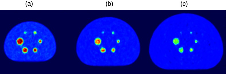
Variability in heterogeneity metrics was investigated for five lesion sizes (13, 17, 22, 28, and 37 mm) and three phantom sizes (850, 1030, and 1200 mm). Larger phantoms demonstrated increased noise due to lower activity concentration. (a) 850 mm, (b) 1030 mm, (c) 1200 mm.
Similarly, the sensitivity of textural metrics due to differences in reconstruction parameters such as iteration number and filtration were investigated (Fig. 3). This simulates the effect of comparing data from multicenter or single-institution trials in the absence of protocol standardization and harmonization. For the sensitivity study, images with high iteration OSEM reconstruction with increased filtration (6 iterations, 28 subsets, 8.6 mm FWHM filtration) were investigated in addition to the reference method. Fifty independent realizations were analyzed for each reconstruction.
Fig. 3.

Representative simulated images for the investigated ordered subsets expectation maximization reconstruction cases: (a) (reference case): 2 iteration, 28 subset, 5 mm FWHM filtration and (b) 6 iteration, 28 subset, 8.6 mm FWHM filtration.
2.4. Power Analysis
To evaluate the impact of quantitative variability in image textural features on statistical powering of clinical trials, sample size calculations were performed. Samples were estimated from a fixed Type I Error rate following Bonferroni correction for multiple hypothesis testing (), a fixed Type II Error rate (, ), and two effect sizes relevant to quantitative PET for treatment response assessment adapted from PERCIST and EORTC guidelines (effect size of 30% and 15%, respectively).31,32 The coefficient of variation (COV) (standard deviation divided by mean) in each image textural feature was measured from the 50 independent phantom image realizations. These input parameters yielded the minimum sample size required to detect statistically significant differences in population mean image textural features via two sample t-test for different lesion and phantom sizes. Quartiles and ranges of sample sizes across the distribution of 35 features listed in Table 1 are reported. Additionally, the impact of phantom girth on sample size is reported.
3. Results
3.1. Simulation Data and Impact of Lesion Size
Mean and standard deviation for histogram and textural feature metrics for the 50 independent realizations of the reference 850 mm phantoms are shown in Table 2 as a function of lesion size. Variability can be depicted in a “radiomics array” (Fig. 4), which plots the value of each metric for each individual realization as a percent difference from the average of the 50 realizations. Complex trends are evident as a function of individual metrics and lesion size. For example, the neighborhood difference metric GLND_strg (strength) shows increasing variability with decreasing lesion size (up to 45% for the 13-mm lesion, up to 35% for the 22-mm lesion, and up to 15% for the 37-mm lesion). Conversely, metrics such as zone percentage do not appreciably change as a function of lesion size.
Table 2.
Mean and standard deviation of intensity histogram and textural features for 50 independent realizations of the 850 mm phantom as a function of lesion size. GLND metrics were not calculable for 13 mm lesion due to insufficient voxels to form a 3×3×3 matrix.
| Lesion size | 37 mm | 28 mm | 22 mm | 17 mm | 13 mm |
|---|---|---|---|---|---|
| GLIH_sd | |||||
| GLIH_skew | |||||
| GLIH_kurt | |||||
| GLIH_engy | |||||
| GLIH_entr | |||||
| GLND_coar | – | ||||
| GLND_cont | – | ||||
| GLND_busy | – | ||||
| GLND_cplx | – | ||||
| GLND_strg | – | ||||
| GLCO_autoc | |||||
| GLCO_contr | |||||
| GLCO_corr | |||||
| GLCO_cprom | |||||
| GLCO_dissi | |||||
| GLCO_energ | |||||
| GLCO_entro | |||||
| GLCO_maxpr | |||||
| GLCO_sosvh | |||||
| GLCO_savgh | |||||
| GLCO_svarh | |||||
| GLCO_senth | |||||
| GLCO_dvarh | |||||
| GLCO_denth | |||||
| GLZS_sze | |||||
| GLZS_lze | |||||
| GLZS_lgze | |||||
| GLZS_hgze | |||||
| GLZS_szlge | |||||
| GLZS_szhge | |||||
| GLZS_lzlge | |||||
| GLZS_lzhge | |||||
| GLZS_glnu | |||||
| GLZS_zsnu | |||||
| GLZS_zp |
Fig. 4.
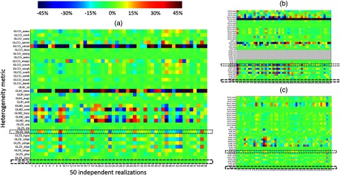
Radiomics array depicting variability in heterogeneity metrics. Each box represents the value of a single metric for one simulated image (850-mm phantom shown). Colormap represents percent difference of individual value relative to the mean of the 50 realizations. Individual metrics exhibit complex trends in variability as a function of object size; for example, variability in large gray zone emphasis (dotted box) increases for smaller lesions, while variability in zone percentage (dashed box) is not a strong function of lesion size: (a) percent difference from mean, 22-mm sphere, (b) percent difference from mean, 13-mm sphere, and (c) percent difference from mean, 37-mm sphere.
Figure 5 depicts COV for the metrics under investigation as a function of lesion size for the case of the reference phantom. The COV was useful to compare variability over the dataset because the dynamic range of means was large (from to for the 850-mm phantom). The COV of the standard deviation of the intensity histogram of each independent realization ranged from 0.03 to 0.05 for the five lesion sizes. The COV of the standard deviation serves as a convenient benchmark for performance of the other metrics because the characteristics of SD are well known. It can be seen that the majority of metrics (24/35) had greater COV over the 50 realizations than the COV of standard deviation for these realizations. One outlier case, skewness, had COV of 0.76 and 1.04 for the 28- and 22-mm lesions; the absolute values of skewness were near zero due to the symmetry of the investigated lesions, which implies that the COV involved division of near-zero means. Metrics with COV similar to or less than standard deviation included: for intensity histogram, energy, and entropy; for co-occurrence matrices, dissimilarity, energy, entropy, sum entropy, and difference entropy; and for zone size, short zone emphasis, large zone emphasis, ZSNU, and zone percentage. In general, the class of metrics with the largest COV due to stochastic variation was the neighborhood difference metrics. Additionally, for nearly all metrics, a trend toward greater COV for smaller lesions was evident.
Fig. 5.
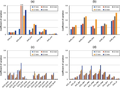
Coefficient of variation for histogram and textural features varies as a function of individual metric and lesion size for the 850-mm phantom. The majority of metrics have COV (absolute value shown) greater than standard deviation, and the class of features with greatest COV on average is the neighborhood difference features (note: starred skewness values overrange the axis to 0.76 and 1.04 due to division of near-zero means): (a) intensity histogram metrics, (b) neighborhood difference metrics, (c) co-occurrence metrics, and (d) size zone metrics.
3.2. Impact of Patient Size
Table 3 shows percent differences of means for metrics calculated at different phantom sizes. Trends as a function of class of metrics were evident. For features of the intensity histogram, standard deviation was relatively insensitive to change in phantom size and corresponding change in image noise (percent difference on order of 5% and 10% for medium and large phantom comparisons). Relative to standard deviation energy and entropy also demonstrated low variability. However, skewness and kurtosis demonstrated large variability as defined as percent difference of mean values. While kurtosis showed variation on the order of 15% and 30% for the medium and large phantom comparisons, percent differences in means for skewness were above 100% for some lesions due to division by near-zero values.
Table 3.
Variable robustness to variation in stochastic noise due to phantom size between and within different classes of heterogeneity metrics with no change to underlying texture.
| Lesion size | Percent difference: 1030 mm to 850 mm | Percent difference: 1200 mm to 850 mm | ||||||||
|---|---|---|---|---|---|---|---|---|---|---|
| 37 mm | 28 mm | 22 mm | 18 mm | 13 mm | 37 mm | 28 mm | 22 mm | 18 mm | 13 mm | |
| GLIH_sd | ||||||||||
| GLIH_skew | 132.3% | 9.6% | 0.2% | 135.2% | 11.3% | |||||
| GLIH_kurt | 6.7% | 0.9% | ||||||||
| GLIH_engy | 2.4% | 2.4% | 0.3% | 2.8% | 6.1% | 6.1% | 2.7% | 5.1% | ||
| GLIH_entr | 0.6% | 0.8% | ||||||||
| GLND_coarse | 23.7% | 13.7% | 5.3% | 4.5% | – | 35.9% | 29.3% | 23.5% | 20.2% | – |
| GLND_contrast | 39.8% | 26.9% | 22.5% | – | 97.0% | 52.7% | 34.0% | – | ||
| GLND_busyness | – | – | ||||||||
| GLND_complexity | 24.9% | 18.7% | 12.3% | – | 56.8% | 32.4% | 14.2% | – | ||
| GLND_strength | 47.2% | 44.1% | 31.2% | 2.8% | – | 94.3% | 85.3% | 86.4% | 33.3% | – |
| GLCO_autoc | 0.4% | 5.8% | 0.4% | 16.7% | ||||||
| GLCO_contr | ||||||||||
| GLCO_corr | 0.1% | |||||||||
| GLCO_cprom | ||||||||||
| GLCO_dissi | ||||||||||
| GLCO_energ | 0.0% | 0.0% | 0.1% | 0.2% | 0.0% | 0.1% | ||||
| GLCO_entro | 0.3% | 0.0% | 0.0% | 0.0% | 0.0% | 0.4% | 0.0% | 0.0% | 0.0% | 0.0% |
| GLCO_maxpr | 2.2% | 0.8% | 8.0% | 1.6% | 0.9% | |||||
| GLCO_sosvh | 4.0% | 12.0% | ||||||||
| GLCO_savgh | 0.5% | 3.1% | 0.5% | 8.4% | ||||||
| GLCO_svarh | 0.2% | 5.3% | 0.0% | 15.7% | ||||||
| GLCO_senth | 0.9% | 0.0% | 0.0% | 1.4% | 0.0% | |||||
| GLCO_dvarh | ||||||||||
| GLCO_denth | ||||||||||
| GLZS_sze | 0.2% | 0.2% | 0.4% | 0.1% | ||||||
| GLZS_lze | 0.4% | 0.8% | 1.2% | 0.0% | 0.9% | 4.3% | ||||
| GLZS_lgze | 16.0% | 10.4% | 5.3% | 30.0% | 23.9% | 11.8% | ||||
| GLZS_hgze | 0.8% | 6.2% | 2.1% | 18.0% | ||||||
| GLZS_szlge | 14.3% | 10.6% | 4.0% | 28.6% | 22.7% | 10.7% | ||||
| GLZS_szhge | 0.9% | 5.8% | 2.3% | 17.1% | ||||||
| GLZS_lzlge | 16.4% | 13.9% | 7.5% | 30.9% | 26.4% | 13.8% | ||||
| GLZS_lzhge | 0.8% | 7.5% | 1.7% | 21.8% | ||||||
| GLZS_glnu | 2.3% | 2.1% | 0.8% | 2.5% | 6.3% | 5.7% | 3.1% | 2.6% | ||
| GLZS_zsnu | 1.0% | 0.8% | 1.8% | 0.4% | ||||||
| GLZS_zp | 0.5% | 0.3% | 0.8% | 0.1% | ||||||
The neighborhood difference matrices demonstrated greatest variability due to simulated patient girth, on the order of 5% to 50% for medium phantom comparisons and 10% to 100% for large phantom comparisons (Fig. 4). Strength and contrast demonstrated greatest variability while busyness and coarseness demonstrated less variability. Variability was greater for larger lesions (e.g., when comparing medium phantoms to small phantoms, strength had variability of 47.2% for 37-mm lesions, 44.1% for 28-mm lesions, 31.2% for 22-mm lesions, and 2.8% for 17-mm lesions) and larger phantoms. For all metrics, percent differences as a function of phantom size were greater than the percent differences of standard deviation.
Co-occurrence metrics demonstrated the most complex behavior for variation in means as a function of phantom size. Metrics such as correlation, energy and entropy had small differences in means between phantom sizes (less than 5%) while autocorrelation, cluster prominence and sum variance had larger differences in means (up to 25%). Six of 14 metrics had less variability in their means than standard deviation.
Zone size metrics such as zone percentage, short zone emphasis and ZSNU showed low levels of variability between phantom sizes (less than 5%). The gray-level emphasis metrics, such as low gray-level zones emphasis and large-zones high gray-level emphasis, demonstrated greater variability up to 16% and 31% for the medium and large phantom comparisons, respectively. Similar to the neighborhood difference metrics, variability was greatest for the largest lesions. Five of 11 metrics demonstrated less variability in their means than standard deviation.
3.3. Impact of Reconstruction
Table 4 shows percent differences of means for metrics calculated for different image reconstructions. In general, variability between the high iteration, high smoothing and low iteration, low smoothing images was on the same order of magnitude to that seen in the comparison of the 1030 to 850 mm phantom sizes. Again, textural features such as skewness of the intensity histogram, contrast, complexity, and strength of the neighborhood difference matrix, autocorrelation and cluster prominence of the co-occurrence matrix, and the gray zone emphasis subset of the zone size matrix demonstrated greatest variability.
Table 4.
Variable robustness to variation in reconstruction parameters between and within different classes of heterogeneity metrics with no change to underlying texture.
| Lesion size | Percent difference: 6 iteration to 2 iteration | ||||
|---|---|---|---|---|---|
| 37 mm | 28 mm | 22 mm | 18 mm | 13 mm | |
| GLIH_sd | |||||
| GLIH_skew | 2.0% | 104.3% | |||
| GLIH_kurt | 0.6% | 10.6% | 11.1% | ||
| GLIH_engy | 4.0% | 4.5% | 1.7% | 3.1% | 2.8% |
| GLIH_entr | |||||
| GLND_coarse | 1.7% | 5.7% | 3.8% | – | |
| GLND_contrast | – | ||||
| GLND_busyness | 4.8% | – | |||
| GLND_complexity | – | ||||
| GLND_strength | – | ||||
| GLCO_autoc | 7.1% | 9.2% | 12.2% | 19.0% | 13.9% |
| GLCO_contr | |||||
| GLCO_corr | 0.4% | 0.4% | |||
| GLCO_cprom | |||||
| GLCO_dissi | |||||
| GLCO_energ | 1.4% | 0.4% | 0.1% | 0.1% | 0.1% |
| GLCO_entro | 0.0% | 0.0% | 0.0% | 0.0% | |
| GLCO_maxpr | 5.1% | 0.9% | 5.0% | 3.8% | 1.9% |
| GLCO_sosvh | 6.5% | 8.6% | 11.0% | 16.3% | 11.0% |
| GLCO_savgh | 3.8% | 5.1% | 6.8% | 10.0% | 7.2% |
| GLCO_svarh | 7.0% | 9.1% | 11.9% | 18.3% | 13.3% |
| GLCO_senth | 0.0% | ||||
| GLCO_dvarh | |||||
| GLCO_denth | |||||
| GLZS_sze | 0.0% | ||||
| GLZS_lze | 2.5% | 1.6% | 2.8% | 1.5% | |
| GLZS_lgze | |||||
| GLZS_hgze | 7.0% | 9.8% | 13.1% | 19.1% | 14.1% |
| GLZS_szlge | |||||
| GLZS_szhge | 6.4% | 9.3% | 13.0% | 17.7% | 13.8% |
| GLZS_lzlge | |||||
| GLZS_lzhge | 10.5% | 12.0% | 13.2% | 24.6% | 15.2% |
| GLZS_glnu | 2.8% | 3.9% | 1.8% | 1.4% | 1.5% |
| GLZS_zsnu | 0.2% | ||||
| GLZS_zp | 0.1% | ||||
Box plot comparisons between absolute values of textural features as a function of patient girth and reconstruction are shown in Fig. 6. Complex differences can be appreciated as a function of lesion size, simulated patient girth, and reconstruction with variable behavior between metrics. For example, entropy of the intensity histogram and busyness of the neighborhood difference matrix showed increasing trends as a function of lesion size and do not vary widely as a function of patient girth or reconstruction. Conversely, skewness of the intensity histogram and coarseness of the neighborhood difference matrix showed decreasing trends as a function of patient size and are generally more sensitive to changes in patient girth and reconstruction.
Fig. 6.

Comparison of sensitivity of textural features to simulated patient girth (left column) and image reconstruction (right column). Metrics display complex behavior as a function of simulated lesion size, phantom size, and reconstruction. Box plots indicate median, quartiles, minimum, and maximum of the 50 realizations for each metric.
In Fig. 7, variability in the means of the 50 simulations as a function of patient size and reconstruction is shown for the neighborhood difference metrics. This may represent, for example, the expected difference in average values of metrics between a theoretical multicenter trial in which injected activities or reconstructions were not standardized. Variability of the ND metrics, which generally fall within the upper quartile of the investigated metrics for variability, was up to 40% for the comparison of the 1030 and 850 mm phantoms and the comparison of the high iteration, high filtration and low iteration, low filtration reconstructions. For the comparison of the 1200 and 850 mm phantoms, variability was up to 100% despite no difference in the underlying ground truth image. Additionally, trends in variability as a function of lesion size were evident with variability being increased for larger lesions.
Fig. 7.
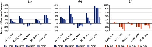
Effects of simulated phantom girth and reconstruction on the mean of the 50 independent realizations of neighborhood difference metrics. While trends vary between sensitivity studies, in general strength, contrast, and complexity exhibit greatest percent difference between means while busyness and coarseness exhibit lower percent difference. The reference case is a girth of 850 mm with 2 iteration reconstruction: (a) 1030 to 850 mm (2 iteration), (b) 1200 to 850 mm (2 iteration), and (c) 6 iteration to 2 iteration (850 mm).
3.4. Power Analyses and Implications for Clinical Trials
Variability estimates were extended to estimation of sample size for theoretical clinical trials. Table 5 depicts the number of patients required to power a study with 95% confidence to detect an effect size of 30% and 15% as a function of individual textural feature. Note that these numbers are inherently conservative because they assume variability only due to the investigated stochastic effects. Results are shown as a function of the ranking of metrics within their distribution and large variability in theoretical patient numbers is evident as a function of metric. For instance, the median sample size across all metrics was 5 to 7 patients for a 30% effect and 10 to 17 patients for a 15% effect, depending on lesion size. However, the metric with the maximum variability due only to stochastic effects (skewness of the intensity histogram) required a theoretical dataset up to hundreds to thousands of patients. As described previously, skewness shows erratic behavior because the symmetry of the lesions results in values very near zero. Additionally, the data similarly showed a trend of larger studies being necessary to elucidate clinical effects in smaller lesions.
Table 5.
Representative number of patients to power for clinical effect size of 30% or 15% due only to stochastic variability. Results are reported for metrics which correspond to the minimum, first quartile, median, third quartile, and maximum of the respective distributions.
| 30% effect size | 15% effect size | ||||||||
|---|---|---|---|---|---|---|---|---|---|
| 37 mm | 28 mm | 22 mm | 17 mm | 37 mm | 28 mm | 22 mm | 17 mm | ||
| Min | 3 | 3 | 3 | 3 | Min | 3 | 3 | 3 | 3 |
| Q1 | 3 | 3 | 3 | 4 | Q1 | 4 | 5 | 5 | 6 |
| Median | 5 | 5 | 6 | 7 | Median | 10 | 10 | 14 | 17 |
| Q3 | 6 | 6 | 10 | 14 | Q3 | 13 | 16 | 30 | 44 |
| Max | 22 | 313 | 587 | 52 | Max | 80 | 1244 | 2337 | 200 |
Similar analysis can be applied to demonstrate the change in estimated sample size as a function of patient girth. Table 6 shows the estimated sample size for the neighborhood difference metrics, which generally fell within the upper quartile of variability in the overall distribution across lesion sizes and patient sizes. However, trends in ranking of other metrics were not easily described; for example, the zone size metrics had variable rankings across the remaining three quartiles for differing lesion size and patient size.
Table 6.
Change in number of patients required for clinical effect size of 30% as a function of patient girth for neighborhood difference metrics.
| Small girth (850 mm) | Large girth (1200 mm) | ||||||||
|---|---|---|---|---|---|---|---|---|---|
| 37 mm | 28 mm | 22 mm | 17 mm | 37 mm | 28 mm | 22 mm | 17 mm | ||
| Coarseness | 6 | 9 | 9 | 12 | Coarseness | 10 | 15 | 21 | 38 |
| Contrast | 13 | 15 | 34 | 38 | Contrast | 19 | 21 | 62 | 88 |
| Busyness | 10 | 11 | 7 | 27 | Busyness | 11 | 15 | 12 | 73 |
| Complexity | 11 | 11 | 16 | 14 | Complexity | 12 | 13 | 28 | 41 |
| Strength | 22 | 25 | 38 | 52 | Strength | 24 | 38 | 66 | 126 |
The differences in image noise in realizations of the two phantoms led to a large difference in the theoretical study size. For instance, powering a study for a 30% effect size in coarseness might require 6 to 12 patients due only to stochastic variability if 10 mCi were injected into patients 850 mm in girth, but 10 to 38 patients if 10 mCi were injected into patients 1200 mm in girth. These findings are a direct consequence of poorer counting statistics in larger patients due to increased photon attenuation and scatter.
4. Discussion
In this study, we investigated the impact of fundamental imaging parameters on textural features, including acquisition noise, lesion size, phantom size, and reconstruction method. Substantial and feature-dependent patterns of variability between individual realizations were observed despite no change in the underlying true image values.
The success of using textural feature metrics in clinical research or clinical practice will depend on the quantitative accuracy of the imaging and analysis procedures. This accuracy depends on several factors not considered here, including but not limited to inter- and intrasite protocol variability, inter- and intramanufacturer scanner variability, scanner calibration, dependence on ancillary equipment such as dose calibrators, and other factors.33 Many of these elements are addressed by the QIBA Profile for FDG-PET/CT imaging.34 However, these results reveal that there are sources of variability that can confound studies attempting to link textural feature metrics to biomarkers or clinical outcomes outside of those expected to be controlled using QIBA profile guidelines. The implication of these trends in variability is that patient studies that are appropriately designed to compensate for stochastic variation for one metric or class of metrics may not be appropriate for all metrics. For example, many more patients may be required to evaluate significant clinical effects in the neighborhood difference metrics than in the subset of zone size metrics that includes short zone emphasis, large zone emphasis, ZSNU, and zone percentage.
The investigated textural features demonstrated several orders of magnitude of variability in COV. Some of these trends could be expressed as a function of class, such as neighborhood difference metrics having greater variability than most other metrics, but in many cases these relationships cannot be easily described due to differences in the composition of the textural matrices and the complexity of the mathematical forms of the metrics. In extreme cases, such as skewness of the intensity histogram, COV was dramatically increased on the order of 0.7 to 1.0. Most metrics demonstrated greater variability for smaller lesions and reduced variability for larger lesions. This is likely due to the greater impact of noise on image values for distributions containing small numbers of voxels. It is noted that COV is only one aspect of the utility of a metric intended for correlation to clinical outcomes, and that low COV does not imply that a metric is useful.
For the sensitivity study in patient girth, means of neighborhood difference metrics were different by up to 40% when comparing images of the 850-mm phantom to the 1030-mm phantom and up to 100% when comparing images of the 850-mm phantom to the 1200-mm phantom. For the sensitivity study in reconstruction, variability when comparing high iteration, high filtration, and low iteration, low filtration OSEM reconstruction was of similar magnitude to the 1030 to 850 mm girth comparisons. In both sensitivity studies, metrics such as skewness of the intensity histogram, contrast, complexity, and strength of the neighborhood difference matrix, autocorrelation and cluster prominence of the co-occurrence matrix, and the gray zone emphasis subset of the zone size matrix showed large variation despite no change in the underlying ground truth image, and percent differences tended to be larger for larger lesions.
A handful of prior investigations of quantitative radiomics in the patient setting have been performed17–22 and our simulation studies appear to be in concordance with these results. For instance, in the test-retest study of 20 patients by Galavis et al.,17 a maximum variability of approximately 30% to 50% was observed for coarseness, while in our study variability up to 40% was observed purely as a function of changing the phantom girth from the 5th percentile for males to the 80th percentile. Similarly, skewness had a maximum variability of 200% in the patient study of Galavis et al.,17 well within the variability seen in our simulations of patient size. Metrics with low variability in our study, such as energy, entropy, zone percentage, and ZSNU have previously been reported to have low variability in studies of patient data.17,19,22
A limitation in this study is the use of uniform objects in the phantom design. For example, the symmetric geometry of the lesions resulted in very low values of the skewness of the intensity histogram, such that small changes in the histogram due to stochastic effects led to large percent differences in mean values between phantom sizes. An asymmetric lesion, then, might show less variability in skewness due to stochastic effects. However, the variability of skewness in the test-retest study of Galavis et al.17 was similar to our simulated results, suggesting that symmetric phantoms are acceptable models for at least some patient data. Further investigation into morphological features of lesions may provide insight into the limitations of certain textural features, particularly in the context of longitudinal imaging studies for therapeutic response assessment. Additionally, the NEMA phantom geometry is most relevant to body imaging, with high-activity lesions up to 37 mm surrounded by low activity background, and different geometries may be more appropriate to applications such as imaging in very low activity background (i.e., lung), imaging very large lesions, or imaging hypointense lesions. Analysis of realistic heterogeneity from patient images, incorporation of this data into simulations, and development of physical phantoms with known heterogeneity are future directions for this work.
A second limitation of this study is that we did not consider the calculation of the metrics. In other words, how do we know that the individual calculations are correct, or that the calculation of the same metrics in other publications is correct? Intuitively, this might seem to matter only for very complex calculations, but we have recently shown that even simple calculations (e.g., mean, maximum, minimum, and standard deviation) by FDA-approved commercial analysis software contain substantial errors.35 There are several reasons why results between studies may disagree due to calculation differences, such as straightforward mistakes in algorithms or coding, lack of consistency in metric specifications (e.g., as described in Orlhac et al.19), and ambiguities in free parameters used for metric calculations (e.g., the gray level discretization or the size of the neighborhood difference matrix). We did not address these limitations because there is not yet a standard for testing or comparing the calculation of image texture metrics, such as the QIBA digital reference object35 which is intended for metric validation. When combined with the observed variation in many textural features as described above, there is a clear need for a reference test prior to an evaluation of the studies using similar metrics.
The overarching message of this study is that different metrics and classes of metrics that are commonly used in PET heterogeneity studies have different behaviors due to only to basic patient and imaging properties, including acquisition noise, lesion size, patient size, and image reconstruction method. These trends may have implications for statistical testing, modeling, and correlation to clinical endpoints using textural features and compound upon the existing problems of radiomics analysis in small datasets, such as bias in significance or regression due to multiple hypothesis testing. Furthermore, these data indicate a methodology to investigate the quantitative aspects of clinical trials utilizing textural feature analysis using simulations, which complements other methods such as phantom and test-retest studies.
5. Conclusion
The sensitivity of PET textural features to basic variations in image acquisition and processing can be large and is feature-dependent. Realistic image simulations represent an effective method of investigating the sensitivity of these metrics to many image parameters, such as the effect of patient girth and reconstruction, and augment other methods such as phantom studies and test-retest patient studies. While reference standards have recently become available for quantitative imaging, additional standards are needed for textural analysis to ensure that prospective trials that incorporate PET textural features are sufficiently well-designed to detect biologically driven responses to treatments and to predict clinical outcomes.
Acknowledgments
We thank Larry Pierce, Adam Alessio, and William Yuh for helpful discussions and review. Supported by NIH grants R01 CA169072, U01 CA148131, NCI Contract (SAIC-Frederick) 24XS036-004, and a research contract from GE Healthcare.
Biographies
Matthew J. Nyflot is an assistant professor in the Department of Radiation Oncology at the University of Washington and is certified by the American Board of Radiology in therapeutic medical physics. He received his PhD in medical physics from the University of Wisconsin in 2011. His primary research interest is in the application of quantitative imaging to personalized cancer therapy.
Fei Yang has been a therapeutic medical physics resident in the Department of Radiation Oncology at the University of Washington since 2013. His current research interest lies in quantitative imaging with emphasis on tumor phenotypic heterogeneity characterization and prognosis prediction.
Darrin Byrd received his BA degree in physics from the University of California, Berkeley, in 2005 and his MS degree in physics from the University of Wisconsin, Milwaukee, in 2010. He has worked in the Imaging Research Laboratory at the University of Washington since 2011. Currently, he is involved in numerous efforts in positron emission tomography/computed tomography (PET/CT) quantitation, including improvements to calibration methods, algorithm performance, and clinical practices.
Stephen R. Bowen is an assistant professor in the Departments of Radiation Oncology and Radiology at the University of Washington. He received his PhD in medical physics from the University of Wisconsin in 2011. His current research interests include quantitative molecular imaging for personalized radiation oncology treatment strategies, as well as multimodal imaging characterization of cancer heterogeneity.
George A. Sandison is a professor of medical physics and vice chair for medical physics, Department of Radiation Oncology, University of Washington. He received his PhD in physics in 1987 and has held administrative and academic positions at several universities in Canada and the USA. His research interests include problems in radiation therapy treatment, including radiation dose computation and optimization, motion management, and the biological modeling of radiation therapy.
Paul E. Kinahan is a professor and vice chair for research in the Department of Radiology, University of Washington, with joint appointments in physics and bioengineering. He is director of UWMC PET/CT imaging physics and head of the imaging research laboratory. He received his PhD in bioengineering in 1994 at the University of Pennsylvania. His research interests include the physics of PET/CT imaging, statistical image reconstruction, optimization of PET/CT image quality, and quantitative imaging to improve therapies.
References
- 1.Lambin P., et al. , “Radiomics: extracting more information from medical images using advanced feature analysis,” Eur. J. Cancer 48(4), 441–446 (2012). 10.1016/j.ejca.2011.11.036 [DOI] [PMC free article] [PubMed] [Google Scholar]
- 2.Aerts H. J., et al. , “Decoding tumour phenotype by noninvasive imaging using a quantitative radiomics approach,” Nat. Commun. 5(4006), 1–8 (2014). [DOI] [PMC free article] [PubMed] [Google Scholar]
- 3.Byrd D., Linden H., Kinahan P. E., “Efforts addressing SUV accuracy for pet quantitation and standardization,” SNMMI PET Cent. Excellence Newsl. 10(4), 1–3 (2013). [Google Scholar]
- 4.Rosenkrantz A. B., et al. , “Clinical utility of quantitative imaging,” Acad. Radiol. 22(1), 33–49 (2015). 10.1016/j.acra.2014.08.011 [DOI] [PMC free article] [PubMed] [Google Scholar]
- 5.Kessler L. G., et al. , “The emerging science of quantitative imaging biomarkers terminology and definitions for scientific studies and regulatory submissions,” Stat. Methods Med. Res. 24(1), 9–26 (2014). [DOI] [PubMed] [Google Scholar]
- 6.Haralick R. M., Shanmugam K., Dinstein I. H., “Textural features for image classification,” IEEE Trans. Syst. Man Cybern. 3(6), 610–621 (1973). 10.1109/TSMC.1973.4309314 [DOI] [Google Scholar]
- 7.Amadasun M., King R., “Textural features corresponding to textural properties,” IEEE Trans. Syst. Man Cybern. 19(5), 1264–1274 (1989). 10.1109/21.44046 [DOI] [Google Scholar]
- 8.Thibault G., Angulo J., Meyer F., “Advanced statistical matrices for texture characterization: application to cell classification,” IEEE Trans. Biomed. Eng. 61(3), 630–637 (2014). 10.1109/TBME.2013.2284600 [DOI] [PubMed] [Google Scholar]
- 9.Vaidya M., et al. , “Combined PET/CT image characteristics for radiotherapy tumor response in lung cancer,” Radiother. Oncol. 102(2), 239–245 (2012). 10.1016/j.radonc.2011.10.014 [DOI] [PubMed] [Google Scholar]
- 10.Tixier F., et al. , “Intratumor heterogeneity characterized by textural features on baseline 18F-FDG PET images predicts response to concomitant radiochemotherapy in esophageal cancer,” J. Nucl. Med. 52(3), 369–378 (2011). 10.2967/jnumed.110.082404 [DOI] [PMC free article] [PubMed] [Google Scholar]
- 11.Cook G. J., et al. , “Are pretreatment 18F-FDG PET tumor textural features in non-small cell lung cancer associated with response and survival after chemoradiotherapy?,” J. Nucl. Med. 54(1), 19–26 (2013). 10.2967/jnumed.112.107375 [DOI] [PubMed] [Google Scholar]
- 12.Tan S., et al. , “Spatial-temporal [(1)(8)F]FDG-PET features for predicting pathologic response of esophageal cancer to neoadjuvant chemoradiation therapy,” Int. J. Radiat. Oncol. Biol. Phys. 85(5), 1375–1382 (2013). 10.1016/j.ijrobp.2012.10.017 [DOI] [PMC free article] [PubMed] [Google Scholar]
- 13.Bundschuh R. A., et al. , “Textural parameters of tumor heterogeneity in 18F-FDG PET/CT for therapy response assessment and prognosis in patients with locally advanced rectal cancer,” J. Nucl. Med. 55(6), 891–897 (2014). 10.2967/jnumed.113.127340 [DOI] [PubMed] [Google Scholar]
- 14.Soussan M., et al. , “Relationship between tumor heterogeneity measured on FDG-PET/CT and pathological prognostic factors in invasive breast cancer,” PLoS One 9(4), e94017 (2014). 10.1371/journal.pone.0094017 [DOI] [PMC free article] [PubMed] [Google Scholar]
- 15.El Naqa I., et al. , “Exploring feature-based approaches in PET images for predicting cancer treatment outcomes,” Pattern Recognit. 42(6), 1162–1171 (2009). 10.1016/j.patcog.2008.08.011 [DOI] [PMC free article] [PubMed] [Google Scholar]
- 16.Cheng N. M., et al. , “Zone-size nonuniformity of (18)F-FDG PET regional textural features predicts survival in patients with oropharyngeal cancer,” Eur. J. Nucl. Med. Mol. Imaging 42(3), 419–428 (2015). 10.1007/s00259-014-2933-1 [DOI] [PubMed] [Google Scholar]
- 17.Galavis P. E., et al. , “Variability of textural features in FDG PET images due to different acquisition modes and reconstruction parameters,” Acta Oncol. 49(7), 1012–1016 (2010). 10.3109/0284186X.2010.498437 [DOI] [PMC free article] [PubMed] [Google Scholar]
- 18.Tixier F., et al. , “Reproducibility of tumor uptake heterogeneity characterization through textural feature analysis in 18F-FDG PET,” J. Nucl. Med. 53(5), 693–700 (2012). 10.2967/jnumed.111.099127 [DOI] [PMC free article] [PubMed] [Google Scholar]
- 19.Orlhac F., et al. , “Tumor texture analysis in 18F-FDG PET: relationships between texture parameters, histogram indices, standardized uptake values, metabolic volumes, and total lesion glycolysis,” J. Nucl. Med. 55(3), 414–422 (2014). 10.2967/jnumed.113.129858 [DOI] [PubMed] [Google Scholar]
- 20.Hatt M., et al. , “FDG PET uptake characterization through texture analysis: investigating the complementary nature of heterogeneity and functional tumor volume in a multi-cancer site patient cohort,” J. Nucl. Med. (2014). 10.2967/jnumed.114.144055 [DOI] [PubMed]
- 21.Yip S., et al. , “Comparison of texture features derived from static and respiratory-gated PET images in non-small cell lung cancer,” PLoS One 9(12), e115510 (2014). 10.1371/journal.pone.0115510 [DOI] [PMC free article] [PubMed] [Google Scholar]
- 22.Hatt M., et al. , “Robustness of intratumour (1)(8)F-FDG PET uptake heterogeneity quantification for therapy response prediction in oesophageal carcinoma,” Eur. J. Nucl. Med. Mol. Imaging 40(11), 1662–1671 (2013). 10.1007/s00259-013-2486-8 [DOI] [PubMed] [Google Scholar]
- 23.Comtat C., et al. , “Simulating whole-body PET scanning with rapid analytical methods,” in IEEE Nuclear Science Symp. Conf. Record, Vol. 1263, pp. 1260–1264 (1999). [Google Scholar]
- 24.University of Washington Imaging Research Laboratory, “ASIM PET simulator,” http://depts.washington.edu/asimuw/ (17 June 2012).
- 25.NEMA Standards Publication NU 2-2012: Performance Measurements of Positron Emission Tomographs, National Electrical Manufacturers Association, Washington, DC: (2013). [Google Scholar]
- 26.Manjeshwar R. M., et al. , “Fully 3D PET iterative reconstruction using distance-driven projectors and native scanner geometry,” in Nuclear Science Symp. Conf. Record, 2006, pp. 2804–2807, IEEE; (2006). [Google Scholar]
- 27.Sun C., Wee W. G., “Neighboring gray level dependence matrix for texture classification,” Comput. Vision Graphics Image Process. 23(3), 341–352 (1983). 10.1016/0734-189X(83)90032-4 [DOI] [Google Scholar]
- 28.Soh L. K., Tsatsoulis C., “Texture analysis of SAR sea ice imagery using gray level co-occurrence matrices,” IEEE Trans. Geosci. Remote Sens. 37(2), 780–795 (1999). 10.1109/36.752194 [DOI] [Google Scholar]
- 29.Yang F., et al. , “Temporal analysis of intratumoral metabolic heterogeneity characterized by textural features in cervical cancer,” Eur. J. Nucl. Med. Mol. Imaging 40(5), 716–727 (2013). 10.1007/s00259-012-2332-4 [DOI] [PMC free article] [PubMed] [Google Scholar]
- 30.McDowell M. A., et al. , “Anthropometric reference data for children and adults: United States, 2003–2006,” Natl Health Stat Report 10, pp. 1–48 (2008). [PubMed]
- 31.Young H., et al. , “Measurement of clinical and subclinical tumour response using [18F]-fluorodeoxyglucose and positron emission tomography: review and 1999 EORTC recommendations. European Organization for Research and Treatment of Cancer (EORTC) PET Study Group,” Eur. J. Cancer 35(13), 1773–1782 (1999). 10.1016/S0959-8049(99)00229-4 [DOI] [PubMed] [Google Scholar]
- 32.Wahl R. L., et al. , “From RECIST to PERCIST: Evolving Considerations for PET response criteria in solid tumors,” J. Nucl. Med. 50S1, 122S–150S (2009). 10.2967/jnumed.108.057307 [DOI] [PMC free article] [PubMed] [Google Scholar]
- 33.Kinahan P. E., Fletcher J. W., “PET/CT standardized uptake values (SUVs) in clinical practice and assessing response to therapy,” Semin. Ultrasound CT MRI 31(6), 496–505 (2010). 10.1053/j.sult.2010.10.001 [DOI] [PMC free article] [PubMed] [Google Scholar]
- 34.FDG-PET/CT Technical Committee, “FDG-PET/CT as an imaging biomarker measuring response to cancer therapy, quantitative imaging biomarkers alliance, Version 1.05,” Publicly Reviewed Version, QIBA, http://rsna.org/QIBA.aspx (11 December 2013).
- 35.Pierce L., et al. , “A digital reference object for the analysis of PET SUV calculation accuracy,” Radiology, Epub ahead of print (2015). [DOI] [PMC free article] [PubMed]