A Comparative Analysis of Reduced Arterial Models for Hemodynamic Monitoring

Abstract

We performed a comparative analysis of reduced arterial models. These models are characterized by a few parameters that can be uniquely estimated from the limited measurements often available in practice. Hence, they offer a means to improve hemodynamic monitoring. We specifically describe Windkessel, transmission-line, and recursive difference equation models, show how they are related, pinpoint their capabilities and limitations, and review how we have applied them for less invasive cardiac output monitoring.

I. Introduction

Mathematical modeling of arterial hemodynamics has been longstanding. Arterial models ranging from extremely simple to highly complex have been developed. The simple or reduced models help us understand the most crucial facets of the physiology. Further, these models are characterized by only a few parameters that can be reliably estimated from the limited measurements typically available in practice. Hence, the reduced models afford a practical framework for personalized hemodynamic monitoring. Several types of reduced arterial models have proven useful in this regard including Windkessel, transmission-line, and recursive difference equation models. In this paper, we describe these models, show how they are related, pinpoint their capabilities and limitations in representing the arterial tree, and give examples of how we have applied them in an attempt to achieve less invasive cardiac output (CO) monitoring.

II. Reduced Arterial Models

A. Windkessel Models

Windkessel models fall under the category of lumped-parameter models (i.e., models characterized by a finite set of elements). The most popular Windkessel model accounts for the total arterial compliance (C) of the large arteries and the total peripheral resistance (R) of the small arteries (Fig. 1a). Thus, this model regards the arterial tree as a single reservoir and predicts exponential diastolic blood pressure (BP) decays with a time constant equal to τ = RC (Fig. 1b). The model transfer function relating CO (q(t)) to BP (p(t)) (i.e., arterial impedance) in the Laplace-domain is as follows:

$$\frac{\mathrm{P}(\mathrm{s})}{\mathrm{Q}(\mathrm{s})}=\frac{\mathrm{R}}{1+\text{sRC}}$$ (1)

Fig. 1.

(a), (c) Windkessel models of the arterial tree. (b) These models predict exponential diastolic blood pressure (BP) decays.

Windkessel models with more than two elements have also been proposed to improve predictive capacity. For example, the three-element Windkessel model (Fig. 1c) provides some improvement in representing the transfer function over the higher frequency regime.

B. Transmission-Line Models

Transmission-line models are within the category of distributed models (i.e., models characterized by an infinite set of elements). Hence, these models regard the arterial tree as spatially dispersed, infinitesimal reservoirs of different BP levels due to finite pulse wave velocity.

A popular transmission-line model is a parallel connection of m ideal, lossless transmission-lines terminated by three-parameter Windkessels (Fig. 2a). One of multiple interpretations of the lines and loads [1] is as follows. Each line represents the wave travel path between the central aorta and a peripheral artery. A line of length (x_i) accounts for the inertance (L_0i) and compliance (C_0i) of the large arteries. So, it has constant characteristic impedance (Z_ci= √(L_0i/C_0i)) and allows waves to travel with constant pulse transit time (T_di= √(L_0iC_0i)). Each terminal load represents the arterial bed distal to the peripheral artery. A load accounts for the resistance (R_i, Z_ci) and compliance (C_i) of the small arteries. Hence, it has frequency-dependent impedance (Z_i(ω)) while matching the line impedance at infinite frequency.

Fig. 2.

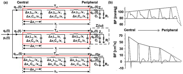
(a) Transmission-line model of the arterial tree. (b) This model predicts the progressive distortion that BP and blood flow rate (BF) waveforms undergo with increasing distance from the heart.

Waves traveling on each transmission-line in the forward direction are reflected at the terminal load (i.e., the site of impedance mismatch) in the backward direction according to the reflection coefficient (Γ_i(ω)=(Z_i(ω)−Z_ci)/(Z_i(ω)+Z_ci)). The BP and blood flow rate (BF) at any point on a line thus arises by adding or subtracting the waves after time shifting to account for the pulse transit time. In this way, the model predicts the progressive distortion that BP and BF waveforms undergo with increasing distance from the heart (Fig. 2b).

The model transfer functions relating central BP (p_c(t)) to peripheral BP (p_pi(t)) and p_c(t) to CO (q_c(t)) (i.e., inverse of arterial impedance) in the Laplace-domain are as follows:

$$\frac{{\mathrm{P}}_{\text{pi}}(\mathrm{s})}{{\mathrm{P}}_{\mathrm{c}}(\mathrm{s})}=\frac{\mathrm{s}+\frac{1}{{\mathrm{R}}_{\mathrm{i}}{\mathrm{C}}_{\mathrm{i}}}+\frac{1}{{\mathrm{Z}}_{\text{ci}}{\mathrm{C}}_{\mathrm{i}}}}{\left(\mathrm{s}+\frac{1}{{\mathrm{R}}_{\mathrm{i}}{\mathrm{C}}_{\mathrm{i}}}+\frac{1}{2{\mathrm{Z}}_{\text{ci}}{\mathrm{C}}_{\mathrm{i}}}\right){\mathrm{e}}^{{\text{sT}}_{\text{di}}}+\frac{1}{2{\mathrm{Z}}_{\text{ci}}{\mathrm{C}}_{\mathrm{i}}}{\mathrm{e}}^{-{\text{sT}}_{\text{di}}}}$$ (2)

$$\frac{{\mathrm{Q}}_{\mathrm{c}}(\mathrm{s})}{{\mathrm{P}}_{\mathrm{c}}(\mathrm{s})}=\sum _{\mathrm{i}=1}^{\mathrm{m}}\frac{1}{{\mathrm{Z}}_{\text{ci}}}\frac{\left(\mathrm{s}+\frac{1}{{\mathrm{R}}_{\mathrm{i}}{\mathrm{C}}_{\mathrm{i}}}+\frac{1}{2{\mathrm{Z}}_{\text{ci}}{\mathrm{C}}_{\mathrm{i}}}\right){\mathrm{e}}^{{\text{sT}}_{\text{di}}}-\frac{1}{2{\mathrm{Z}}_{\text{ci}}{\mathrm{C}}_{\mathrm{i}}}{\mathrm{e}}^{-{\text{sT}}_{\text{di}}}}{\left(\mathrm{s}+\frac{1}{{\mathrm{R}}_{\mathrm{i}}{\mathrm{C}}_{\mathrm{i}}}+\frac{1}{2{\mathrm{Z}}_{\text{ci}}{\mathrm{C}}_{\mathrm{i}}}\right){\mathrm{e}}^{{\text{sT}}_{\text{di}}}+\frac{1}{2{\mathrm{Z}}_{\text{ci}}{\mathrm{C}}_{\mathrm{i}}}{\mathrm{e}}^{-{\text{sT}}_{\text{di}}}}$$ (3)

While this model may not appear to be reduced, these transfer functions reveal its simplicity. That is, the first transfer function is characterized by only three parameters (i.e., R_iC_i, Z_ciC_i, and T_di), while the second transfer function is represented with eight parameters for the popular “T-tube” configuration in which m = 2.

C. Recursive Difference Equation Models

Recursive difference equation models lie under the category of black-box models (i.e., models characterized by parameters without any physical meaning). Black-box models thus assume little about the arterial tree.

Recursive difference equation models regard the present value of the output of a system to be determined by values of the input and past values of the output. The most popular model is linear with constant parameters as follow:

$$\mathrm{y}[\mathrm{n}]=-\sum _{\mathrm{k}=1}^{\mathrm{p}}{\mathrm{a}}_{\mathrm{k}}\mathrm{y}[\text{n-k}]+\sum _{\mathrm{k}=0}^{\mathrm{q}}{\mathrm{b}}_{\mathrm{k}}\mathrm{x}[\text{n-k}]$$ (4)

Here, n is discrete-time, x[n] and y[n] are the input and output of a system, {a_k, b_k} are sets of parameters that define the system transfer function (as shown in Eq. (5)), and p and q determine the number of these parameters (model order). The non-physical parameters can only be ascertained by fitting a measured input to a measured output. The number of parameters that can be estimated is restricted by the number of frequency components in the measurements. Since these components are limited in practice, this model can only be characterized by relatively few parameters. The model thus predicts the system output by design.

Due to its black-box nature, this model is general and could conceivably represent any sub-system of the arterial network. For example, the system could represent the arterial impedance whose input and output are CO and BP.

The model transfer function relating the input to output in the Z-domain is as follows:

$$\frac{\mathrm{Y}[\mathrm{z}]}{\mathrm{X}[\mathrm{z}]}=\frac{{\displaystyle \sum _{\mathrm{k}=0}^{\mathrm{q}}}{\mathrm{b}}_{\mathrm{k}}{\mathrm{z}}^{-\mathrm{k}}}{1+{\displaystyle \sum _{\mathrm{k}=1}^{\mathrm{p}}}{\mathrm{a}}_{\mathrm{k}}{\mathrm{z}}^{-\mathrm{k}}}$$ (5)

Hence, the only assumption of the model transfer function is that it takes on pole-zero form in the Z-domain.

III. Model Relationships

The reduced arterial models may appear distinct, but they are related to each other. We show these relationships below.

To relate the transmission-line model (Fig. 2a) to the Windkessel model (Fig. 1a), we let the frequency ω in the former model decrease towards zero. Since large artery characteristic impedance (Z_ci= √(L_0i/C_0i)) is usually in the range of 0.1 mmHg-sec/ml, the inductors in the line short before the line capacitors open. Further, assuming small artery compliance (C_i) is much less than large artery compliance (C_0i), the load capacitor opens before the line capacitors. So, at low frequencies, each line becomes a single capacitor with compliance C_0i, while each load becomes a single resistor with resistance Z_ci+R_i. The parallel connection of all m of these RC circuits is another RC circuit with resistance $\mathrm{R}=\left[1/{\sum }_{\mathrm{i}=1}^{\mathrm{m}}\left(\frac{1}{{\mathrm{Z}}_{\text{ci}}+{\mathrm{R}}_{\mathrm{i}}}\right)\right]$ and compliance $\mathrm{C}={\sum }_{\mathrm{i}=1}^{\mathrm{m}}{\mathrm{C}}_{0\mathrm{i}}$. Thus, the transmission-line model reduces to the Windkessel model as the frequency decreases.

To relate the transmission-line model to the recursive difference equation model (Eq. (5)), we transform the transfer functions of the former model (Eqs. (2) and (3)) to the Z-domain as follows:

$$\frac{{\mathrm{P}}_{\text{pi}}[\mathrm{z}]}{{\mathrm{P}}_{\mathrm{c}}[\mathrm{z}]}=\frac{\left({\mathrm{f}}_{\mathrm{s}}+\frac{1}{{\mathrm{R}}_{\mathrm{i}}{\mathrm{C}}_{\mathrm{i}}}+\frac{1}{{\mathrm{Z}}_{\text{ci}}{\mathrm{C}}_{\mathrm{i}}}\right)-{\mathrm{f}}_{\mathbf{s}}{\mathrm{z}}^{-1}}{\left({\mathrm{f}}_{\mathrm{s}}+\frac{1}{{\mathrm{R}}_{\mathrm{i}}{\mathrm{C}}_{\mathrm{i}}}+\frac{1}{2{\mathrm{Z}}_{\text{ci}}{\mathrm{C}}_{\mathrm{i}}}\right){\mathrm{z}}^{{\mathrm{T}}_{\text{di}}}-{\mathrm{f}}_{\mathbf{s}}{\mathrm{z}}^{{\mathrm{T}}_{\text{di}}-1}+\frac{1}{2{\mathrm{Z}}_{\text{ci}}{\mathrm{C}}_{\mathrm{i}}}{\mathrm{z}}^{-{\mathrm{T}}_{\text{di}}}}$$ (6)

$$\frac{{\mathrm{Q}}_{\mathrm{c}}[\mathrm{z}]}{{\mathrm{P}}_{\mathrm{c}}[\mathrm{z}]}=\sum _{\mathrm{i}=1}^{\mathrm{m}}\frac{1}{{\mathrm{Z}}_{\text{ci}}}\frac{\left({\mathrm{f}}_{\mathrm{s}}+\frac{1}{{\mathrm{R}}_{\mathrm{i}}{\mathrm{C}}_{\mathrm{i}}}+\frac{1}{2{\mathrm{Z}}_{\text{ci}}{\mathrm{C}}_{\mathrm{i}}}\right){\mathrm{z}}^{{\mathrm{T}}_{\text{di}}}-{\mathrm{f}}_{\mathrm{s}}{\mathrm{z}}^{{\mathrm{T}}_{\text{di}}-1}-\frac{1}{2{\mathrm{Z}}_{\text{ci}}{\mathrm{C}}_{\mathrm{i}}}{\mathrm{z}}^{-{\mathrm{T}}_{\text{di}}}}{\left({\mathrm{f}}_{\mathrm{s}}+\frac{1}{{\mathrm{R}}_{\mathrm{i}}{\mathrm{C}}_{\mathrm{i}}}+\frac{1}{2{\mathrm{Z}}_{\text{ci}}{\mathrm{C}}_{\mathrm{i}}}\right){\mathrm{z}}^{{\mathrm{T}}_{\text{di}}}-{\mathrm{f}}_{\mathrm{s}}{\mathrm{z}}^{{\mathrm{T}}_{\text{di}}-1}+\frac{1}{2{\mathrm{Z}}_{\text{ci}}{\mathrm{C}}_{\mathrm{i}}}{\mathrm{z}}^{-{\mathrm{T}}_{\text{di}}}}$$ (7)

where f_s is the sampling frequency. Thus, the Z-domain transfer functions of the transmission-line model are of pole-zero form but with parameters that have physical meaning. The recursive difference equation model can thus be viewed as a generalization of the transmission-line model.

Since recursive difference equation models can capture the behavior of transmission-line models, the former models with input and output of CO and BP may likewise reduce to the Windkessel model as the frequency declines. Also, note that the Z-domain transfer function of the Windkessel model (Fig. 1a) can be easily shown to be of first-order pole-zero form.

IV. Model Capabilities and Limitations

The reduced arterial models have different capabilities and limitations in terms of what aspects of arterial hemodynamics they can and cannot represent. We elaborate below.

Windkessel models account for the reservoir (i.e., volume storage) behavior of the arterial tree. On the other hand, by assuming a single reservoir or, equivalently, infinite pulse wave velocity, these models cannot mimic the differences in BP and BF that occur between various sites in the arterial tree (Fig. 2b). However, as implied above, the Windkessel model (Fig. 1a) is a good representation of the arterial tree at low frequencies. At such frequencies, the wavelengths of the traveling waves are long (i.e., wavelength equals pulse wave velocity divided by frequency) relative to the dimension of the arterial tree such that BP and BF at its various sites converge to the same levels (i.e., it becomes one reservoir).

Windkessel models are also a good representation of the central BP waveform as evidenced by the exponential diastolic decays often apparent in this waveform (Figs. 1b and 2b). Noordergraaf provides the following explanation [2]. Forward and backward waves in the aorta have large phasic differences due to the long and varying distances between the aorta and the main reflection sites at the arterial terminations. So, waves with short wavelengths tend to cancel each other out. But, waves with longer wavelengths constructively add. The key point again is that the arterial tree acts more like a single reservoir with increasing wavelengths. We add to this explanation by noting that waves with short wavelengths constructively add in the periphery due to the close proximity to the arterial terminations. Thus, exponential diastolic decays are obscured in peripheral BP waveforms (Fig. 2b).

In sum, Windkessel models are representative of central but not peripheral BP waveforms and low frequency BP variations regardless of their site of measurement.

Transmission-line models assume finite pulse wave velocity and thus account for high frequency wave reflection. Further, they reduce to the Windkessel model (Fig. 1a) at low frequencies. So, these models are representative of central and peripheral BP waveforms. Thus, by accounting for both reservoir and finite pulse wave velocity behaviors, transmission-line models may be considered as unifying arterial models. In other words, two different models to account for these behaviors [3]are unnecessary.

However, the transmission-line model (Fig. 2a) ignores elastic and geometric tapering and multi-level branching. As we discussed in [1], these assumptions can be defended to some degree as follows. As Noordergraaf stated, the arterial terminations are often the main reflection sites. One reason is that they offer the largest impedance mismatch, as the radius of the arterioles is much smaller than that of the proximal arteries. Another reason is that vessel tapering tends to be offset by vessel branching in the forward direction such that relative impedance matching is obtained. On the other hand, backward waves are expected to experience strong re-reflections as they return towards the heart due to necessarily significant impedance mismatch in this direction. Further, the multiple reflected waves that return from the periphery actually interact in the aorta due to multi-level branching.

Recursive difference equation models can likewise account for reservoir and finite pulse wave velocity behaviors, so these models may also be regarded as unifying models. Further, the models are not physically based and thus make few assumptions about the arterial tree. Note that at the same time, the pole-zero form of the recursive difference equation model (Eq. (5)) can be considered to be justified by the physical transmission-line model (Fig. 2a). However, the trade-off is that their parameters carry no physical meaning.

V. Less Invasive Co Monitoring Applications

Due to their simplicity, these arterial models can often be identified (i.e., their parameters can be uniquely estimated) from the limited information in the waveforms measured in a patient monitoring setting (e.g., the ICU). The parameter estimates can provide value above and beyond the measured waveforms about a patient’s hemodynamic status. Many investigators have employed these models for this purpose. For example, we have used them as a basis for estimating relative CO change from a peripheral BP waveform in order to achieve continuous and minimally or non-invasive invasive CO tracking [4, 5]. We review these efforts below.

High frequency wave reflection profoundly impacts the shape of peripheral BP waveforms and thus constitutes a serious challenge in CO estimation (Fig. 2b). We conceived two techniques to overcome the confounding wave reflection.

The idea of the first technique is to bypass the confounding wave reflection by exploiting the fact that the Windkessel model dominates at low frequencies. So, for example, peripheral BP would eventually decay like a pure exponential with τ = RC once the faster wave reflection vanishes.

The technique thus estimates the pure exponential decay that would eventually result if the heart suddenly stopped beating by analyzing a peripheral BP waveform over many beats (Fig. 3a). First, the BP response to a single heartbeat is estimated (h(t) in Fig. 3a). Then, τ is determined from the tail end of h(t) once the faster wave reflection dissipates (Fig. 3a). Finally, assuming constant C, proportional CO is computed as the ratio of mean BP (MAP) and τ.

Fig. 3.

Techniques for estimating relative cardiac output (CO) change from a peripheral BP waveform based on (a) recursive difference equation (Eq. (5)) and Windkessel models and (b) transmission-line and Windkessel models.

To estimate the single heartbeat BP response, an impulse train (x(t)) is formed in which each impulse is located at the foot of the BP waveform (y(t)) and is scaled by the ensuing pulse pressure (PP). Then, the impulse response (h(t), time-domain version of transfer function) is estimated, which when convolved with x(t), optimally fits y(t). By definition, h(t) represents the BP response to a single heartbeat.

The impulse response h(t) is identified via the recursive difference equation model (Eq. (5)). The parameter sets {a_k, b_k}, which define h(t), are estimated, for a fixed model-order, via the closed-form linear least squares solution [6]. The model order is determined by minimizing the minimum description length criterion over a set of candidate orders [6].

Interestingly, this model assumes that the BP waveform arises as an impulse train convolved with a pole-zero system. This system can be thought of as a cascade connection of three transfer functions relating: (1) the impulse train to the CO waveform (Q_c(z)/X(z)); (2) the CO waveform to the central BP waveform (P_c(z)/Q_c(z)); and (3) the central BP waveform to the peripheral BP waveform (P_pi(z)/P_c(z)). The impulse response of transfer function (1) is proportional to one beat of the CO waveform. We have empirically found that it can often be represented as a second-order pole-zero system. The transmission-line model (Fig. 2a) indicates that that transfer functions (2) and (3) can also be represented as pole-zero systems (Eqs. (6) and (7)). Thus, the BP model is essentially justified by the physical model. Note that this reasoning parallels the justification of the all-pole model of speech via a physical vocal tract model [7].

The idea of the second technique is to attenuate the confounding wave reflection by capitalizing on the fact that it hardly impacts the shape of the central BP waveform. So, first, the central BP waveform is estimated from a peripheral BP waveform. Then, an exponential is fitted to the diastolic decay of the estimated waveform to determine τ (Fig. 1b). Finally, proportional CO is computed as MAP divided by τ.

To estimate the central BP waveform, the transmission-line model (Fig. 2a) is employed. First, the transfer function relating the peripheral BP waveform (p_pi(t)) to the central BP waveform (p_c(t)) is defined in terms of three model parameters (inverse of Eq. (7) and Fig. 3b). These parameters are estimated by exploiting the fact that central aortic BF is negligible during diastole. That is, the transfer function relating p_pi(t) to the component of the CO waveform that reaches the peripheral artery measurement site (q_ci(t)) is defined in terms of the same parameters (Fig. 3b). The common parameters are then estimated by finding the BP-to-BF transfer function, which when applied to p_pi(t), optimally fits a scaled q_ci(t) to zero during diastole (Fig. 3b). Since the physical parameters are constrained (e.g., 0 < Z_ciC_i < R_iC_i), this optimization is achieved via a numerical search. Finally, the BP-to-BP transfer function with the parameter estimates is applied to p_pi(t) to estimate p_c(t) (Fig. 3b).

Experimental testing of both techniques is described elsewhere (e.g., [4, 5, 8]).

VI. Conclusion

In summary, we have described a set of reduced models of arterial hemodynamics. While these models are all related, they have distinct capabilities and limitations. In particular, the Windkessel model (Fig. 1a) can represent the central BP waveform and low frequency BP variations but cannot account for peripheral BP waveforms. The transmission-line model (Fig. 2a) and the recursive difference equation model (Eq. (5)) can represent both central and peripheral BP waveforms including low frequency BP variations. However, the former model neglects some aspects of the arterial tree, while the latter model does not carry any physical meaning. We and others have estimated the relatively few parameters of all of these models from limited waveforms to improve hemodynamic monitoring. Thus, each of these models is useful, and the proper model choice depends on the particular hemodynamic monitoring application at hand.

References

- 1.Zhang G. Tube-Load Model Parameter Estimation for Monitoring Arterial Hemodynamics. Frontiers in Computational Physiology And Medicine. 2012 Nov;:15–64. doi: 10.3389/fphys.2011.00072. [DOI] [PMC free article] [PubMed] [Google Scholar]
- 2.Noordergraaf A. Circulatory System Dynamics. New York: Academic Press; 1978. [Google Scholar]
- 3.Hughes A. The Reservoir-wave Paradigm. Journal of Hypertension. 2012 Sep;30(9):1880–1881. doi: 10.1097/HJH.0b013e3283560960. [DOI] [PubMed] [Google Scholar]
- 4.Mukkamala R. Continuous Cardiac Output Monitoring by Peripheral Blood Pressure Waveform Analysis. IEEE Transactions on Biomedical Engineering. 2006 Mar;53(3) doi: 10.1109/TBME.2005.869780. [DOI] [PubMed] [Google Scholar]
- 5.Zhang G. Early Detection of Hemorrhage via Central Pulse Pressure Derived from a Non-Invasive Peripheral Arterial Blood Pressure Waveform. IEEE EMBC Conference; 2012. pp. 3116–3119. [DOI] [PubMed] [Google Scholar]
- 6.Ljung L. System Identification: Theory for the User. Upper Saddle River, NJ: Prentice Hall PTR; c1999. [Google Scholar]
- 7.Rabiner L. Digital Processing of Speech Signals. Prentice-Hall; 1978. [Google Scholar]
- 8.Reisner A. Monitoring non-invasive cardiac output and stroke volume during experimental human hypovolaemia and resuscitation. Brit J Anaesthesia. 2011;106(1):23–30. doi: 10.1093/bja/aeq295. [DOI] [PMC free article] [PubMed] [Google Scholar]