Quantitative Ultrasound Comparison of MAT and 4T1 Mammary Tumors in Mice and Rats Across Multiple Imaging Systems

Abstract

Objectives

Quantitative ultrasound estimates such as the frequency-dependent backscatter coefficient (BSC) have the potential to enhance noninvasive tissue characterization and to identify tumors better than traditional B-mode imaging. Thus, investigating system independence of BSC estimates from multiple imaging platforms is important for assessing their capabilities to detect tissue differences.

Methods

Mouse and rat mammary tumor models, 4T1 and MAT, respectively, were used in a comparative experiment using 3 imaging systems (Siemens, Ultrasonix, and VisualSonics) with 5 different transducers covering a range of ultrasonic frequencies.

Results

Functional analysis of variance of the MAT and 4T1 BSC-versus-frequency curves revealed statistically significant differences between the two tumor types. Variations also were found among results from different transducers, attributable to frequency range effects. At 3 to 8 MHz, tumor BSC functions using different systems showed no differences between tumor type, but at 10 to 20 MHz, there were differences between 4T1 and MAT tumors. Fitting an average spline model to the combined BSC estimates (3–22 MHz) demonstrated that the BSC differences between tumors increased with increasing frequency, with the greatest separation above 15 MHz. Confining the analysis to larger tumors resulted in better discrimination over a wider bandwidth.

Conclusions

Confining the comparison to higher ultrasonic frequencies or larger tumor sizes allowed for separation of BSC-versus-frequency curves from 4T1 and MAT tumors. These constraints ensure that a greater fraction of the backscattered signals originated from within the tumor, thus demonstrating that statistically significant tumor differences were detected.

Quantitative ultrasound estimates based on the backscatter coefficient (BSC) have demonstrated the ability to detect and classify disease beyond the capabilities of traditional B-mode imaging. Quantitative ultrasound has been able to differentiate live from apoptotic cells or oncotic cells in vitro with high-frequency ultrasound,^1,2 monitor changes in tissue microstructure due to high-intensity focused ultrasound at high frequencies in a preclinical model,³ and monitor changes due to chemotherapy clinically at 6 MHz.⁴ Tumors have been characterized and differentiated using quantitative ultrasound at high frequencies in preclinical models of thyroid cancer,⁵ at high frequencies in clinical applications for ocular tumors,^6,7 and at clinical frequencies in human patients for breast tumors⁸ and prostate cancers.^9,10 Also, the BSC has been proven valuable for diagnosing fatty liver disease clinically¹¹ and for monitoring physiologic and pharmacologic responses in renal function at clinical frequencies in an animal model.^12,13

One of the BSC features that is often cited as an advantage is its system independence; ie, the same BSC value for a given tissue can be estimated from any imaging platform. Previous studies have demonstrated system independence of BSC estimates in well-characterized phantoms.^14–17 These investigations applied single-element imaging systems measuring backscatter levels for strong glass bead scatterer phantoms (1–12 MHz),^14,15 single-element imaging systems for probing weakly scattering agar-in-agar phantoms (1–13 MHz),¹⁶ and clinical array imaging systems for estimating BSC for phantoms with glass bead scatterers (1–15 MHz).¹⁷ Parametric estimates based on the BSC have demonstrated the ability to differentiate different types of orthotopic mouse tumors ex vivo (16–24 MHz),¹⁸ to identify regions of micrometastases within resected lymph nodes clinically (26.5 MHz center),¹⁹ and to identify dominant sources of backscattering in the renal cortex (frequencies covering 2.5–15 MHz).^12,13,20,21 The frequency ranges in these studies cover the range being investigated in this study: namely, from the clinical frequencies to the lower end of the small-animal pre-clinical imaging frequencies, covering, for example, 1 to 21 MHz.

This study addresses the need for demonstrating that in vivo interlaboratory measurements can be used to distinguish different types of tumors, while being able to obtain consistent BSC results from all systems. Previous studies^22,23 examined BSC agreement across single-element and clinical imaging systems for an in vivo rodent fibroadenoma model over a frequency range of 1 to 14 MHz. The heterogeneity of the benign fibroadenomas provided a near worst-case scenario to evaluate quantitative ultrasound performance. The study presented herein seeks to expand on this work using clinical and preclinical array imaging systems to test their capability to detect known tissue differences while maintaining good agreement in BSC values across all systems.

Mouse (4T1) and rat (MAT) mammary tumor models were used in a comparative experiment with 3 array-based ultrasound imaging systems (Siemens, Ultrasonix, and VisualSonics) and 5 different transducers covering a range of frequency bandwidths. Backscatter coefficient agreement between systems was assessed, as well as the ability to differentiate the two tumor types.

Materials and Methods

Animal Models

Mouse and rat orthotopic mammary tumor models were used for a comparison between different tumor types. In the first model, 1 × 10³ 4T1 mouse mammary carcinoma cells (4T1; ATCC CRL-2539; American Type Culture Collection, Manassas, VA) were injected into the right inguinal mammary fat pad of BALB/c mice (Harlan Laboratories, Inc, Indianapolis, IN). In the second model, 1 × 10³ MAT mammary adenocarcinoma cells (13762 MAT B III; ATCC CRL-1666; American Type Culture Collection) were injected into the right abdominal mammary fat pad of Sprague Dawley rats (Harlan Laboratories, Inc). Both cell lines are malignant epithelial cells that form solid tumors with round to oval cells that vary greatly in size. Tumors show abundant and abnormal mitotic figures with minimal extracellular matrix. Regions of ischemic necrosis can be observed, particularly for the MAT tumors, which show regions of spatially separated necrosis that do not typically arise in the 4T1 tumors, likely due to their limited size. Two experimental sessions were performed; during the first session, 12 4T1 tumors were imaged and during the second, 5 4T1 tumors and 10 MAT tumors were imaged. The experimental protocol was approved by the Institutional Animal Care and Use Committee, University of Illinois at Urbana-Champaign, and satisfied all University and National Institutes of Health rules for the humane use of laboratory animals.

Ultrasound Systems

Two clinical and 1 preclinical, array-based ultrasound imagingsystems were used to image the same tumors. The clinical systems were an Ultrasonix RP (Ultrasonix Medical Corporation, Richmond, British Columbia, Canada), and a Siemens Acuson S2000 (Siemens Medical Solutions USA, Inc Malvern, PA). The preclinical system was a VisualSonics Vevo2100 (VisualSonics, Inc, Toronto, Ontario, Canada). For each system, the individual transducers used and their nominal center frequencies are summarized in Table 1.

Table 1.

Summary of Imaging Systems and Transducers

Imaging System	Transducer	Nominal Center Frequency, MHz	Bandwidth Used, MHz
Ultrasonix RP	L14-5/38	6	3–8.5
Siemens Acuson
S2000	9L4	6	3–10.8
	18L6	10	3–10.8
VisualSonics
Vevo2100	MS200	15	8.5–13.3
	MS400	30	8.5–22
	MS550S	40	Image data only

The transducer name, nominal center frequency, and approximate bandwidth over which the data were analyzed are included.

Animal Handling

Both studies were performed at the Bioacoustics Research Laboratory at the University of Illinois at Urbana-Champaign to enable sequential data collection from each animal with each imaging system. During an experiment, an animal was anesthetized by inhaled isoflurane. Hair over the tumor was first shaved and then depilated. The animal was then placed in a custom-built holder so that only the bottom portion of the animal with the tumor was submerged in a tank of 37°C degassed water. The animal remained in the same location for the duration of scanning by all imaging systems. To acquire echo data from approximately the same location within the tumor, each transducer was mounted in a custom holder attached to a micro-positioning system (Daedal; Parker Hannifin Corporation, Irvine, CA). Each transducer was oriented such that ultrasonic scan lines propagated horizontally in identical vertical scan planes, facilitated by the positioning system. Five parallel slices of echo data were acquired with each transducer, separated by up to 1 mm, depending on the tumor size.

Tumors were scanned with each imaging system in a pseudorandom order to avoid any potential biases that could arise due to the length of time under anesthesia. Total scan time for each tumor was approximately 45 minutes, during when the on-site anesthesia level was carefully monitored by a veterinarian (R.J.M.). After imaging with all the transducers, the animal was removed from the water tank and laid in a prone position while a high-resolution 3-dimensional ultrasonic image was acquired with the Vevo2100 using an MS550S probe (nominal center frequency of 40 MHz) to obtain an accurate total volume estimate of the tumor. After imaging, the animals were euthanized, and the tumors were excised and sent to pathology for diagnosis.

Attenuation

Average linear attenuation coefficients were estimated, in separate experiments, using single-element transducers and an insertion loss technique over the bandwidth used in this study¹⁴ for each of the tumor types. Estimates of 0.40 dB/cm-MHz for the 4T1 tumors and 0.71 dB/cm-MHz for the MAT tumors were obtained and used for attenuation compensation in data from the clinical systems.

Backscatter Coefficient

The BSC was calculated for each slice from each transducer using a reference phantom technique.²⁴ The experimental and processing methods have been recently described in detail.²³ Each image slice was divided into analysis windows to calculate the BSC; sizes of the analysis windows are summarized in Table 2. The BSC for each slice was then computed as the average across all analysis windows. If the tumor size was less than approximately 3 analysis windows, then for the smaller tumors, a smaller analysis window was used to allow for a reasonable BSC estimate to be made.

Table 2.

Analysis Window Size and Overlap for Each System

Imaging System	Analysis Window Size		Analysis Window Overlap, %
	Axial	Lateral	Axial	Lateral
Ultrasonix RP	4–10 λ(4T1) 15 λ(MAT)	4–10 λ(4T1) 15 λ(MAT)	75	75
VisualSonics
Vevo2100	10–15 λ	10–15 λ	75	75
Siemens Acuson
S2000	7–15 λ	7–15 λ	75	75

For each system, the wavelength, λ, was calculated based on the nominal center frequency and assumed speed of sound of 1540 m/s.

Statistical Analysis

Detailed statistical analysis methods are described in the “Appendix.”

Results

The imaged tumors were histologically confirmed to be carcinomas (4T1) and adenocarcinomas (MAT). The tumor volumes, measured by segmentation of the 3-dimensional images acquired with the Vevo2100 using onboard software, ranged from 6.3 to 617 mm³ for the 4T1 tumors and from 12.4 to 3096 mm³ for the MAT tumors.

Backscatter Coefficient

Overlap in the transducer bandwidths across several transducers allowed for a direct comparison of the results visually when graphed. Figure 1 shows examples of the average BSCs obtained from 4 4T1 (Figure 1, a–d) and 4 MAT (Figure 1, e–h) tumors. The BSCs for the individual slices for the corresponding tumors are included in the “Appendix” (see Figure A1) to allow for the variability within a tumor and transducer to be observed. A reduction in the interslice and intertransducer variability is observed with the increased tumor volumes (ie, Figure 1, c and d, versus Figure 1, a and b, for the 4T1 tumors and Figure 1, g and h, versus Figure 1, e and f, for the MAT tumors).

Figure 1.

Example BSC curves for 4T1 tumors (a–d) and MAT tumors (e–h). Plots show average BSC curves for all transducers for 4 different 4T1 tumors with volumes of 9.7 (a), 24.6 (b), 75 (c), and 617 (d) mm³ and for 4 different MAT tumors with volumes of 12.4 (e), 88 (f), 133 (g), and 587 (h) mm³. Backscatter coefficient values range from 10⁻⁴ to 10⁻² cm⁻¹ Sr⁻¹ and show variations between transducers. Note that the legend and axes are the same across all BSC graphs presented. (continued)

In Figure 1, c and d, it is illustrated that BSC values for the larger 4T1 tumors are lower than for the smaller 4T1 tumors, with averages between 10⁻⁴ and 10⁻³ cm⁻¹ Sr⁻¹ compared to 10⁻³ and 10⁻² cm⁻¹ Sr⁻¹ for the 4T1 tumors. Less BSC variation between slices and between transducers is also observed for the larger tumors than the smaller tumors (Figure 1, a and b). For the smaller MAT tumors shown in Figure 1, e and f, BSC-versus-frequency curves are relatively flat. Figure 1, e and f, show a larger range of BSC values, equivalent to those observed for similar tumor sizes in the 4T1 tumors. Figure 1, g and h, show BSC values slightly greater than 10⁻⁴ cm⁻¹ Sr⁻¹, similar to the trend observed for 4T1 tumors of similar size in Figure 1, a–d. Backscatter coefficients from larger MAT tumors are shown in Figure 1, g and h, with BSC values ranging from 10⁻² to 10⁻⁴ cm⁻¹ Sr⁻¹. Backscatter coefficient variations between transducers are reduced compared to those observed in the smaller tumors in Figure 1, e and f.

Statistical Analysis

Additional detailed statistical analysis results and graphs are included in the “Appendix.”

Figure 2a presents an average spline curve fit to combined data in this study (all transducers, 13 4T1 tumors, and 8 MAT tumors) for the entire frequency range (3–22 MHz). The spline curves used cubic B-spline basis functions with 20 knots.²⁵ Point-wise 90% confidence intervals are displayed based on 1000 bootstrap samples²⁶ from the BSC curves; all scans for a given tumor and transducer combination were sampled together to account for potential correlation between scans from the same setup. A separation in the average BSC with increased frequency was observed and correlates with the observed statistically significant differences between MAT and 4T1 tumors in the higher frequency band analyzed.

Figure 2.

Overall estimated BSC curves for MAT and 4T1 tumors combining data from all transducers; BSC curves (in decibels) were smoothed using cubic B-spline basis functions with 20 knots covering the range. Ninety percent confidence intervals are displayed. Data are summarized from all tumors (a; 13 4T1 and 8 MAT), tumor volumes greater than 30 mm³ (b; approximate diameter of 3.9 mm; 9 4T1 and 6 MAT), and tumor volumes greater than 70 mm³ (c; approximate diameter of 5.1 mm; 5 4T1 and 6 MAT).

Figure 2b presents the fitted average spline curve restricted to tumors with a computed volume of at least 30 mm³ (approximate diameter of 3.9 mm), whereas Figure 2c presents the fitted average spline curve using only the data from tumors with volume of at least 70 mm³ (approximate diameter of 5.1 mm). In each case, point-wise 90% confidence intervals are also displayed. These are based on 1000 bootstrap samples²⁶ from the BSC curves.

The plots in Figure 2 demonstrate a trend in increasing separation between MAT and 4T1 average BSC spline curves as well as in their confidence intervals as the data are filtered for larger tumor sizes. This trend in the separation may relate to the likelihood of the ultrasonic focal region encompassing more of the tumor as the tumor size increases, thus increasing the likelihood that the scattered signals become more targeted from tumor tissue per se.

Discussion

Both the 4T1 and MAT tumors had a decrease in average BSC values with increased tumor volume, with the larger volumes having less variation across the slices from one transducer and less variation between transducers. At 5 MHz, for example, the BSC for the larger tumors was approximately 10⁻⁴ cm⁻¹ Sr⁻¹, whereas the smaller tumors had BSC values as high as 10⁻² cm⁻¹ Sr⁻¹.

The smoothed curves in Figure 2a show increasing separation between tumor types with increased frequency. However, because there was not a clear separation in 90% confidence intervals and because a decrease in the standard deviation (Std; see “Appendix”) was observed for larger tumors, 2 new plots were constructed using only those tumors whose volumes were greater than 30 mm³ (Figure 2b; BSCs from 9 4T1 and 6 MAT) and for which their volumes were greater than 70 mm³ (Figure 2c; BSCs from 5 4T1 and 6 MAT). The separation between the average BSC curves from the 4T1 and MAT tumors shifted to lower frequencies as the volumes of the tumors increased. There are several factors that likely contributed to this increased BSC separation of tumor types for the larger tumors. First, the range of BSC values decreased with increasing tumor volumes; therefore, limiting the data to the larger tumors also confines the BSCs from individual tumors to lower values. Second, for larger tumors, any effects resulting from inclusion of boundaries, specular reflectors and normal tissue due to the elevational resolution, or limits in segmenting the tumor in plane will likely be lower due to the increased likelihood that the analysis windows would be contained entirely within the tumor boundaries, which would increase the scattered data from tumor tissue per se. For the smallest tumors, the effect of echo signals from outside the tumor would likely contribute to more of the analysis windows. Last, any variations in user outlines would have a great effect in the analyzed tissue. Overall, these summary plots show that with a small increase in tumor volume, the improvements in the separation of the BSC curves between the two tumor types were substantial.

Current clinical imaging systems provide transducers with center frequencies up to 13 MHz for clinical breast imaging. Therefore, the largest separation in differentiating the two types of tumors in this study that is observed above 15 MHz is typically beyond the range used for clinical breast imaging. However, when the analysis was confined to tumors greater than 30 mm³ (corresponding to ≥4 mm in diameter), the BSC began to separate around 10 MHz: that is, within the clinically achievable range.

Although the rodent mammary tumor models used in this study offer a more uniform and simplified tumor architecture compared to the wide variety of tumors encountered clinically, the study demonstrates the level of consistency in making the BSC estimates that is essential for use clinically. Additionally, the ability to begin to differentiate the BSC between these two tumors, which differ subtly from each other, offers the promise of being able to use the BSC to characterize differences in tumor types and, potentially, grades.

Despite the differences in analysis window sizes, system architecture, and transducer characteristics, it was possible to maintain good agreement (no detectable differences between transducers by function analysis of variance (ANOVA) analyses; see “Appendix”) between the BSCs from a tumor type for all systems and transducers. This finding suggests that the BSC is a robust estimate and not sensitive to specific analysis parameters when they are properly taken into account during the analysis.

In conclusion, for a given tumor, it was found that different systems and transducers covering the same frequency range yielded similar BSC-versus-frequency results, in support of BSC system independence. Conversely, comparisons of MAT versus 4T1 tumor BSC-versus-frequency curves within imaging systems indicated that statistically significant tumor differences were detected, supporting the power of the approach for potential diagnostic use. Furthermore, combined analysis of all BSC data across frequencies revealed stronger separation between these two tumor types at the higher frequencies. For the MAT and 4T1 tumor models, better BSC detection of the tumor differences occurred at higher frequencies and for larger tumor volumes. Analysis of the dependence on tumor size suggests that the higher frequencies can separate smaller tumor types more effectively than can the lower frequencies. With larger tumors, even at lower frequencies, BSC results were able to separate the two tumor types effectively, suggesting that the resolution volume versus region of interest size is a critical component of the effectiveness of BSC-based classification of regions of interest.

Abbreviations

ANOVA

analysis of variance

BSC

backscatter coefficient

RMSE

root mean squared error

SNR

signal-to-noise ratio

Std

standard deviation

Appendix

Backscatter Coefficient

Figure A1 shows the BSCs for the individual slices of the corresponding tumors to allow for the variability within a tumor and transducer to be observed.

Statistical Analysis Methods

To compare the BSC variations across the 5 parallel slices of echo data acquired for a single imaging transducer, the Std of the BSC as a function of frequency was calculated. An average of the Std values across all frequencies was calculated. The Std as a function of tumor volume was plotted to evaluate the repeatability of measurements for different-sized tumors. It was conjectured that scans of smaller tumors might include a higher percentage of surrounding tissue than would scans of larger tumors, leading to greater heterogeneity of tissue within the scan, which would be evidenced by a higher level of variability.

As the transducers all had different bandwidths, 2 frequency ranges were selected for the subsequent analyses that allowed for all of the larger range of frequencies to be covered and to ensure all transducers were included. The lower frequency range (3–8.5 MHz) included data from the Ultrasonix and Siemens transducers, and the higher frequency range (8.5–13.5 MHz) included data from the VisualSonics transducers.

To provide an estimate of the difference in magnitude of the BSC estimates between different imaging systems and transducers, a root mean squared error (RMSE) of the logarithm of the BSC-versus-frequency curves between and within systems was calculated. This process enabled an assessment of how the system variation compared to the inherent replication noise level. To calculate the RMSE, the BSC for each transducer was averaged over all slices and at each frequency, after interpolating to the same frequency steps. The logarithm was taken of the BSC, and differences were calculated for all pairs of transducers in the frequency band. The RMSE was then calculated by squaring the difference at each frequency step, averaging across frequencies in the frequency band, and obtaining the root of the resulting error. The maximum RMSEs within and between systems were plotted as a function of tumor volume for each tumor type. For the higher frequency range, only a “within-system” RMSE was calculated. To formally test the capability of the BSC curve to detect tumor differences a functional ANOVA test²⁷ for tumor effect was conducted using the BSC data from each transducer frequency range. Statistical significance was computed via bootstrap resampling.²⁶ The functional signal-to-noise ratio (SNR) for tumor effect was computed²³ for each transducer. To test for possible transducer differences, functional ANOVA was conducted within tumor types and across transducers that covered the lower and higher frequency ranges. Functional ANOVA and functional SNR analyses were necessary because the BSC data consisted of frequency-dependent curves rather than single values; hence, traditional ANOVA methods did not apply to these data.²⁸

Statistical Analysis Results

The Std values of the log-BSC across slices for each transducer and each tumor are plotted in Figure A2a (4T1 tumors) and A2b (MAT tumors). For the Std, a value of 1 corresponds to an order of magnitude in the original BSC estimates. A reduction in the maximum Std was observed with increasing tumor volume, with almost all Std estimates less than 0.4 for tumor volumes greater than 100 smm³ and less than 0.2 for tumor volumes greater than approximately 600 mm³.

The RMSE between the log-scaled BSC curves was computed for each pair of transducers over each of the frequency ranges. The results are summarized in Figure A3, showing the RMSE of the log-BSC for the comparison of both transducers within the same imaging system and between imaging systems over both the low and high frequency ranges used. The highest maximum RMSE values decreased with increased tumor size; ie, a substantial drop in the within-system RMSE is observed around 80 mm³, with a similar trend but less substantial decrease observed for the between-system RMSE.

The functional ANOVA and functional SNR results for detection of tumor differences are summarized in Table A1. There were statistically significant differences between MAT and 4T1 tumors for both VisualSonics transducers and a close P value (.061) for the Siemens 9L4 transducer. The result indicates that the VisualSonics MS200 and MS400 transducers could differentiate between the MAT and 4T1 tumors. Additionally, no statistically significant differences were found for the detection of transducer differences from the functional ANOVA summarized in Table A2. These results indicate that there were no statistically significant detected differences between transducers in a given frequency range. Comparison of functional SNR values in Table A1 versus Table A2 also indicated that the signal for tumor differences was considerably larger than the signal for transducer differences, the latter of which was not statistically significant.

Figure A1.

Individual BSC curves corresponding to the average BSC curves shown in Figure 1. Plots show individual slice BSC for all transducers for 4 different 4T1 tumors with volumes of 9.7 (a), 24.6 (b), 75 (c), and 617 (d) mm³ and for 4 different MAT tumors with volumes of 12.4 (e), 88 (f), 133 (g), and 587 (h) mm³. Backscatter coefficient values range from 10⁻⁴ to 10⁻² cm⁻¹ Sr⁻¹ and show variations between slices and between transducers. Note that the legend and axes are the same across all BSC graphs presented.

Figure A2.

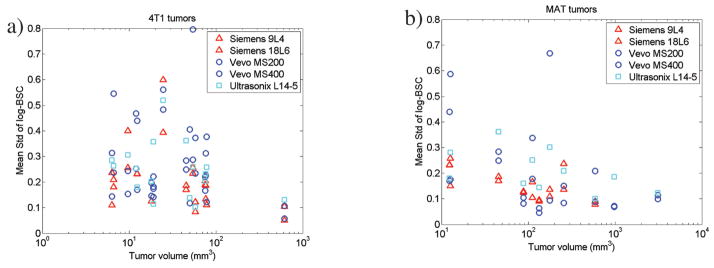
The Std of the log BSC of the 5 slices of data averaged across all frequencies is plotted for each transducer vs the tumor volume. The BSC unit is cm⁻¹ Sr⁻¹. The 4T1 tumors are shown in a, and the MAT tumors are shown in b.

Figure A3.

The maximum RMSE of the log-BSC for each tumor is plotted versus the tumor volume. The BSC unit is cm⁻¹ Sr⁻¹. The between-system RMSE is plotted in blue, and the within-system (transducers from the same imaging system) RMSE is plotted in red.

Table A1.

Functional ANOVA Tests and SNRs for Detection of Tumor Differences (MAT Versus 4T1) for Each of 5 Transducers

Transducer	Frequency Range, MHz	Functional F	P	Residual Std, dB	Functional SNR
Ultrasonix L14-5	3.0–8.5	2.08	.14	5.45	0.10
Siemens 9L4	3.0–10.8	3.47	.061	6.00	0.16
Siemens 18L6	3.0–10.8	0.35	.57	6.18	0.00
VisualSonics MS200	8.5–13.5	5.81	.019a	5.59	0.21
VisualSonics MS400	8.5–21.9	12.49	.0005b	5.48	0.33

P values are based on 2000 bootstrap samples.

^aStatistically significant at level α = .05.

^bStatistically significant at level α = .001.

Table A2.

Functional ANOVA Tests and SNRs for Detection of Transducer Differences for Each Tumor Type

Tumor Type	Frequency Range, MHz	Transducers Compared	Functional F	P	Functional SNR
4T1	3.0–8.5	L14-5, S9L4, S18L6	1.96	.14	0.103
	8.5–13.5	MS200, MS400	1.47	.23	0.060
MAT	3.0–8.5	L14-5, S9L4, S18L6	1.26	.28	0.066
	8.5–13.5	MS200, MS400	1.66	.20	0.091

P values are based on 2000 bootstrap samples.

References

- 1.Kolios MC, Czarnota GJ, Lee M, Hunt JW, Sherar MD. Ultrasonic spectral parameter characterization of apoptosis. Ultrasound Med Biol. 2002;28:589–597. doi: 10.1016/s0301-5629(02)00492-1. [DOI] [PubMed] [Google Scholar]
- 2.Kolios MC, Taggart L, Baddour RE, et al. 2003 IEEE Symposium on Ultrasonics. Piscataway, NJ: Institute of Electrical and Electronic Engineers; 2003. An investigation of backscatter power spectra from cells, cell pellets and microspheres; pp. 752–757. [Google Scholar]
- 3.Sadeghi-Naini A, Papanicolau N, Falou O, et al. Quantitative ultrasound evaluation of tumor cell death response in locally advanced breast cancer patients receiving chemotherapy. Clin Cancer Res. 2013;19:2163–2174. doi: 10.1158/1078-0432.CCR-12-2965. [DOI] [PubMed] [Google Scholar]
- 4.Kemmerer JP, Ghoshal G, Karunakaran C, Oelze ML. Assessment of high-intensity focused ultrasound treatment of rodent mammary tumors using ultrasound backscatter coefficients. J Acoust Soc Am. 2013;134:1559–1568. doi: 10.1121/1.4812877. [DOI] [PMC free article] [PubMed] [Google Scholar]
- 5.Lavarello RJ, Ridgway WR, Sarwate SS, Oelze ML. Characterization of thyroid cancer in mouse models using high-frequency quantitative ultrasound techniques. Ultrasound Med Biol. 2013;39:2333–2341. doi: 10.1016/j.ultrasmedbio.2013.07.006. [DOI] [PMC free article] [PubMed] [Google Scholar]
- 6.Lizzi FL, Ostromogilsky M, Feleppa EJ, Rorke MC, Yaremko MM. Relationship of ultrasonic spectral parameters to features of tissue microstructure. IEEE Trans Ultrason Ferroelectr Freq Control. 1987;34:319–329. doi: 10.1109/t-uffc.1987.26950. [DOI] [PubMed] [Google Scholar]
- 7.Feleppa EJ, Lizzi FL, Coleman DJ, Yaremko MM. Diagnostic spectrum analysis in ophthalmology: a physical perspective. Ultrasound Med Biol. 1986;12:623–631. doi: 10.1016/0301-5629(86)90183-3. [DOI] [PubMed] [Google Scholar]
- 8.Tadayyon H, Sadeghi-Naini A, Wirtzfeld L, Wright FC, Czarnota G. Quantitative ultrasound characterization of locally advanced breast cancer by estimation of its scatterer properties. Med Phys. 2014;41:012903. doi: 10.1118/1.4852875. [DOI] [PubMed] [Google Scholar]
- 9.Balaji KC, Fair WR, Feleppa EJ, et al. Role of Advanced 2 And 3-dimensional ultrasound for detecting prostate cancer. J Urol. 2002;168:2422–2425. doi: 10.1016/S0022-5347(05)64159-6. [DOI] [PubMed] [Google Scholar]
- 10.Feleppa EJ, Kalisz A, Sokil-Melgar JB, et al. Typing of prostate tissue by ultrasonic spectrum analysis. IEEE Trans Ultrason Ferroelectr Freq Control. 1996;43:609–619. [Google Scholar]
- 11.Garra BS, Insana MF, Shawker TH, Wagner RF, Bradford M, Russell M. Quantitative ultrasonic detection and classification of diffuse liver disease: comparison with human observer performance. Invest Radiol. 1989;24:196–203. doi: 10.1097/00004424-198903000-00004. [DOI] [PubMed] [Google Scholar]
- 12.Insana MF, Wood JG, Hall TJ. Identifying acoustic scattering sources in normal renal parenchyma in vivo by varying arterial and ureteral pressures. Ultrasound Med Biol. 1992;18:587–599. doi: 10.1016/0301-5629(92)90073-j. [DOI] [PubMed] [Google Scholar]
- 13.Insana MF, Wood JG, Hall TJ, Cox GG, Harrison LA. Effects of endothelin-1 on renal microvasculature measured using quantitative ultrasound. Ultrasound Med Biol. 1995;21:1143–1151. doi: 10.1016/0301-5629(95)02008-x. [DOI] [PubMed] [Google Scholar]
- 14.Wear KA, Stiles TA, Frank GR. Interlaboratory comparison of ultrasonic backscatter coefficient measurements from 2 to 9 MHz. J Ultrasound Med. 2005;24:1235–1250. doi: 10.7863/jum.2005.24.9.1235. [DOI] [PubMed] [Google Scholar]
- 15.Anderson JJ, Herd MT, King MR, et al. Interlaboratory comparison of backscatter coefficient estimates for tissue-mimicking phantoms. Ultrason Imaging. 2010;32:48–64. doi: 10.1177/016173461003200104. [DOI] [PMC free article] [PubMed] [Google Scholar]
- 16.King MR, Anderson JJ, Herd MT, et al. Ultrasonic backscatter coefficients for weakly scattering, agar spheres in agar phantoms. J Acoust Soc Am. 2010;128:903–908. doi: 10.1121/1.3460109. [DOI] [PMC free article] [PubMed] [Google Scholar]
- 17.Nam K, Rosado-Mendez IM, Wirtzfeld LA, et al. Cross-imaging system comparison of backscatter coefficient estimates from a tissue-mimicking material. J Acoust Soc Am. 2012;132:1319–1324. doi: 10.1121/1.4742725. [DOI] [PMC free article] [PubMed] [Google Scholar]
- 18.Oelze ML, O’Brien WD., Jr Application of three scattering models to characterization of solid tumors in mice. Ultrason Imaging. 2006;28:83–96. doi: 10.1177/016173460602800202. [DOI] [PubMed] [Google Scholar]
- 19.Mamou J, Coron A, Hata M, et al. Three-dimensional high-frequency characterization of cancerous lymph nodes. Ultrasound Med Biol. 2010;36:361–375. doi: 10.1016/j.ultrasmedbio.2009.10.007. [DOI] [PMC free article] [PubMed] [Google Scholar]
- 20.Insana MF, Hall TJ, Wood JG, Yan ZY. Renal ultrasound using parametric imaging techniques to detect changes in microstructure and function. Invest Radiol. 1993;28:720–725. doi: 10.1097/00004424-199308000-00013. [DOI] [PubMed] [Google Scholar]
- 21.Garra BS, Insana MF, Sesterhenn IA, et al. Quantitative ultrasonic detection of parenchymal structural change in diffuse renal disease. Invest Radiol. 1994;29:134–140. doi: 10.1097/00004424-199402000-00002. [DOI] [PubMed] [Google Scholar]
- 22.Wirtzfeld LA, Ghoshal G, Hafez ZT, et al. Comparison of ultrasonic backscatter coefficient estimates from rat mammary tumors using single element and array transducers [abstract] J Acoust Soc Am. 2009;126:2213. [Google Scholar]
- 23.Wirtzfeld LA, Nam K, Labyed Y, et al. Techniques and evaluation from a cross-platform imaging comparison of quantitative ultrasound parameters in an in vivo rodent fibroadenoma model. IEEE Trans Ultrason Ferroelectr Freq Control. 2013;60:1386–1400. doi: 10.1109/TUFFC.2013.2711. [DOI] [PMC free article] [PubMed] [Google Scholar]
- 24.Yao LX, Zagzebski JA, Madsen EL. Backscatter coefficient measurements using a reference phantom to extract depth-dependent instrumentation factors. Ultrason Imaging. 1990;12:58–70. doi: 10.1177/016173469001200105. [DOI] [PubMed] [Google Scholar]
- 25.Chambers JM, Hastie TJ. Chapter 7: Generalized additive models. In: Chambers JM, Hastie TJ, editors. Statistical Models in S. Stamford, CT: Wadsworth & Brooks/Cole; 1992. pp. 249–304. [Google Scholar]
- 26.Elfron B, Tibshirani RJ. An Introduction to the Bootstrap. 1. London, England: Chapman & Hall; 1993. [Google Scholar]
- 27.Shen Q, Faraway J. An F test for linear models with functional responses. Statistica Sinica. 2004;14:1239–1257. [Google Scholar]
- 28.Ramsay JO, Silverman BW. Functional Data Analysis. New York, NY: Springer-Verlag; 1997. [Google Scholar]