Hierarchical Clustering With Prototypes via Minimax Linkage

Abstract

Agglomerative hierarchical clustering is a popular class of methods for understanding the structure of a dataset. The nature of the clustering depends on the choice of linkage—that is, on how one measures the distance between clusters. In this article we investigate minimax linkage, a recently introduced but little-studied linkage. Minimax linkage is unique in naturally associating a prototype chosen from the original dataset with every interior node of the dendrogram. These prototypes can be used to greatly enhance the interpretability of a hierarchical clustering. Furthermore, we prove that minimax linkage has a number of desirable theoretical properties; for example, minimax-linkage dendrograms cannot have inversions (unlike centroid linkage) and is robust against certain perturbations of a dataset. We provide an efficient implementation and illustrate minimax linkage’s strengths as a data analysis and visualization tool on a study of words from encyclopedia articles and on a dataset of images of human faces.

1. INTRODUCTION

Suppose that we are given the pairwise dissimilarities between n objects x₁, …, x_n. Our focus is on a clustering method that can make the relationships among objects in the dataset readily apparent, so that an individual with little statistical knowledge can understand the structure of the data. In many applications, these objects may be vectors in ℝ^p, but for our purposes we require only a matrix of dissimilarities d(x_i, x_j) between objects, not the objects themselves.

Hierarchical clustering methods organize data in the form of trees. Each leaf corresponds to one of the original data points, x_i, and each interior node represents a subset or cluster of points. Agglomerative hierarchical clustering algorithms build trees in a bottom-up approach, beginning with n singleton clusters of the form {x_i}, and then merging the two closest clusters at each stage. This merging is repeated until only one cluster remains. Because at each step two clusters are merged into one cluster, the algorithm terminates after n − 1 steps. The resulting binary tree formed by this process is commonly displayed as a dendrogram by placing each leaf at height 0 and every interior node (corresponding to a merge) at a height equal to the distance between the clusters merged, that is, h(G ∪ H) = d(G, H) (see Figure 1).

Figure 1.

Agglomerative hierarchical clustering produces a sequence of clusterings that can be represented as a dendrogram. Each interior node of the dendrogram corresponds to a merging of two clusters (or points).

An important choice required in agglomerative hierarchical clustering is how to measure the distance between clusters. Common, extensively studied distances between clusters (referred to as “linkages”) include complete, single, average, and centroid (e.g. Everitt, Landau, and Leese 2001; Hastie, Tibshirani, and Friedman 2009). Given two clusters G and H, these are defined as follows:

• Complete: d_C(G, H) = max_g∈G,h∈H d(g, h)

• Single: d_S(G, H) = min_g∈G,h∈H d(g, h)

• Average: $d_A(G,H)=\frac{1}{\mid G\mid \mid H\mid }{\sum }_{\mathbf{g}\in G,\mathbf{h}\in H}d(\mathbf{g},\mathbf{h})$

• Centroid: d_cen(G, H) = d(x̄_G, x̄_H).

In words, complete linkage uses the largest intercluster distance, single linkage the minimum intercluster distance, average linkage the average intercluster distance, and, finally, centroid linkage uses the distance between the centroids of the two clusters.

From a tree, we can recover n possible clusterings, corresponding to each step of the algorithm. To cut the tree at a given height h means to return the last clustering before a merging occurs of two clusters more than h apart. Given a complete linkage tree, cutting at height h gives a clustering in which all points of a cluster are within h of one another; given a single linkage tree, it gives a clustering for which no two clusters have points closer than h from each other.

In a two-page “applications note,” Ao et al. (2005) proposed a new measure of cluster distance, called minimax linkage, for the problem of selecting tag single nucleotide polymorphisms (SNPs). However, beyond a brief empirical study in the context of tag SNP selection, the authors offered little analysis of the measure’s properties and performance. We believe that their proposed linkage has great potential as a tool for data analysis and thus merits closer attention. In this article we show that minimax linkage shares many of the desirable theoretical properties of the standard linkages while adding interpretative value. In Section 2, we define minimax linkage and explain its connection to the set cover problem. We also show how this method naturally produces “prototype-enhanced” dendrograms, thereby increasing the ease of interpretation. In Section 3, we present several theoretical properties of the linkage. In Section 4 we review some related work, and in Section 5 we use two real datasets to demonstrate the appeal of using minimax linkage compared with other linkages. In Section 6 we present an empirical study on both real and simulated datasets. Finally, in Section 7, we discuss algorithmics, presenting an efficient algorithm that we have implemented for this problem and time comparisons to a standard implementation of complete linkage.

2. MINIMAX LINKAGE

We begin with a few definitions that are used throughout the rest of the article. For any point x and cluster C, define

$$d_{max}(\mathbf{x},C)=\underset{{\mathbf{x}}^{\prime }\in C}{max}d(\mathbf{x},{\mathbf{x}}^{\prime })$$

as the distance to the farthest point in C from x. Define the minimax radius of the cluster C as

$$r(C)=\underset{\mathbf{x}\in C}{min}{d}_{max}(\mathbf{x},C);$$ (1)

that is, find the point x ∈ C from which all points in C are as close as possible (i.e., the point whose farthest point is closest). We call this minimizing point the prototype for C. Note that a (closed) ball of radius r(C) centered at the prototype covers all of C. Finally, define the minimax linkage between two clusters G and H as

$$d(G,H)=r(G\cup H);$$ (2)

that is, we measure the distance between clusters G and H by the minimax radius of the resulting merged cluster (see Figure 2). By (2), the height of the interior node corresponding to cluster C is simply r(C). With each node of the tree, we have an associated prototype, namely the most central (in the sense of minimizing d_max) data point of the newly formed cluster. We mentioned earlier that the cutting of complete and single linkage trees admits a simple interpretation. The motivation for minimax linkage is that it also has an appealing interpretation for cuts.

Figure 2.

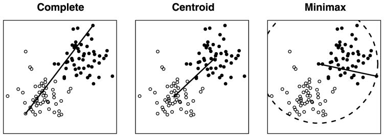
Complete, centroid, and minimax linkages. The solid black line represents the distance between the two clusters according to each linkage. The circle is of radius r(G ∪ H), where G and H denote the two clusters.

Property 1

Cutting a minimax linkage tree at height h yields a clustering, C₁, …, C_k, and a set of prototypes, p₁, …, p_k, in which for every cluster C_i there is a prototype p_i ∈ C_i such that all points in C_i are within h of p_i.

Proof

Let C₁, …, C_k be the clustering when we cut at height h. Then r(C_i) ≤ h. That is, min_x∈Cid_max(x, C_i) ≤ h or, equivalently, there exists a point p_i ∈ C_i such that d_max(p_i, C_i) ≤ h. This implies that every x′ ∈ C_i is within h of p_i.

The foregoing property is the motivation for using this linkage. When performing minimax hierarchical clustering, we can easily retain the prototype index associated with each interior node (n − 1 of them in total). Thus, for each merge we have a single representative data point for the resulting cluster.

For microarray data, it is common to define d(gene₁, gene₂) = 1 − correlation(gene₁, gene₂). Cutting a minimax clustering of the genes at height 1 − ρ₀ yields a dataset of “prototypical” genes in which every gene has correlation of at least ρ₀ with one of the prototype genes. In this sense, every gene in the dataset is guaranteed to be represented in the prototype set. The prototypes of minimax linkage have a close relationship to the set cover problem, which we review next. Consider a set of n balls centered at each x_i and of a fixed radius h. The set cover problem asks for the smallest number of such balls required to cover all of the data points x₁, …, x_n. This is a well-studied NP-hard problem that has been widely applied to clustering. Tipping and Schölkopf (2001) emphasized the fact that the set cover prototypes come with a desirable maximum distortion guarantee (i.e., no point will be farther than h from its prototype). Based on the foregoing property, it is easy to see that for each possible cut, we get a set of prototypes with a maximum distortion guarantee.

Figure 3 shows how we can enhance the information conveyed by a dendrogram by indicating the prototypes associated with each interior node. For example, we see that at the step when there are only two clusters, the points “7” and “9” are chosen as prototypes (a reasonable choice looking at the configuration of points). Of course, for larger n, fitting all n − 1 prototypes onto the dendrogram becomes difficult. In such a case, we propose displaying only the prototypes of a given cut. Figure 4 displays an example that also visually demonstrates the set cover connection of property 1 (the radius of the balls equals the height of the cut).

Figure 3.

A “prototype-enhanced” minimax linkage dendrogram corresponding to the two-dimensional toy dataset shown in the right panel. Every interior node of the dendrogram has an associated prototype that we display. The height of each interior node is the maximum distance of any element in its branch to the prototype.

Figure 4.

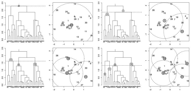
Successive cuts of a dendrogram with prototypes displayed: Cutting at height h yields a set of prototypes (shown in gray) such that every element of the dataset is covered by the set of balls of radius h centered at the prototypes. As h decreases, more prototypes are required.

3. INVERSIONS AND ADMISSIBILITY PROPERTIES

Implicit in the above discussion of dendrograms and cuts is the assumption that there are no inversions—that is, that parent nodes are always higher than their children. A well-known difficulty with centroid linkage is that it can in fact have such inversions (e.g., Everitt, Landau, and Leese 2001). Inversions lead to clumsy rules for visualization and a less obvious interpretation of what it means to cut at a certain height. To be precise, suppose that we are in the middle of forming an agglomerative tree and are considering merging the clusters G and H. Then a linkage does not allow inversions if d(G, H) ≥ max{h(G), h(H)}.

Property 2

Minimax linkage trees do not have inversions.

Proof

Without loss of generality, suppose that h(G) ≥ h(H). We want to show d(G, H) ≥ h(G). This holds trivially if h(G) = 0 (i.e., G is a singleton cluster), so we assume that G = G₁ ∪ G₂ was formed by merging the clusters G₁ and G₂. Let

$${\mathbf{x}}^{\ast }=\underset{\mathbf{x}\in G\cup H}{argmin}{d}_{max}(\mathbf{x},G\cup H)$$

be the prototype of G ∪ H. Suppose that x^* ∈ G_i ∪ H. Then we have

$$\begin{array}{l}h(G)=d(G_1,G_2)\le d(G_i,H)\\ =\underset{\mathbf{x}\in G_i\cup H}{min}{d}_{max}(\mathbf{x},G_i\cup H)\le d_{max}({\mathbf{x}}^{\ast },G_i\cup H)\\ \le d_{max}({\mathbf{x}}^{\ast },G_1\cup G_2\cup H)=r(G\cup H)=d(G,H),\end{array}$$

where the first inequality holds because the algorithm chose to merge G₁ with G₂ rather than either G_i with H. That H was a candidate when G₁ and G₂ were merged follows from our initial assumption that h(G) ≥ h(H).

Fisher and Van Ness (1971) proposed a number of admissibility conditions for hierarchical clustering procedures with the goal of “eliminat[ing] obviously bad clustering algorithms.” Minimax linkage holds up well against the well-known linkages according to these admissibility standards, as we show in what follows.

A linkage is said to be “well-structured k-group admissible,” if whenever there exists a clustering C₁, …, C_k, in which all within-cluster distances are smaller than all between-cluster distances, the hierarchical clustering will produce this clustering after n − k merges.

Property 3

Minimax linkage is “well-structured k-group admissible.”

Proof

Suppose that there exists a partition of the data, C₁, …, C_k, such that d(x, x′) ≤ a if x, x′ ∈ C_i and d(x, x′) > a if x ∈ C_i, x′ ∈ C_j with i ≠ j. It follows that for any x ∈ C_i, d_max(x, C_i) ≤ a and d_max(x, C_j) > a. Now, if G, H ⊂ C_i, then

$$d(G,H)=\underset{\mathbf{x}\in G\cup H}{min}{d}_{max}(\mathbf{x},G\cup H)\le \underset{\mathbf{x}\in G\cup H}{min}{d}_{max}(\mathbf{x},C_i)\le a.$$

Moreover, if G ⊂ C_i and H ⊂{x₁, …, x_n} \ C_i, then

$$d(G,H)=\underset{\mathbf{x}\in G\cup H}{min}{d}_{max}(\mathbf{x},G\cup H)>a$$

since d_max(x, G ∪ H) ≥ d_max(x, H) > a for all x ∈ G and d_max(x, G ∪ H) ≥ d_max(x, G) > a for all x ∈ H. Thus minimax linkage will always merge clusters within a group C_i before merging a cluster G ⊂ C_i with a subset not contained in C_i. This establishes that at some merge in the algorithm, C_i is formed. Now d(C_i, C_j) > a and h(C_i) ≤ a, so cutting at height a gives precisely the clustering C₁, …, C_k. Because this is a k cluster solution, this state is reached after n − k merges.

We list the following two properties without proofs, because they follow immediately from the properties of max and min.

Property 4

Minimax linkage is

• “Monotone admissible”: Monotone transformation of the distances leaves the clustering unchanged.

• “Point proportion admissible”: Duplicating any of the x_i’s has no effect on the clusters formed.

Single and complete linkages are admissible in these senses as well. The latter two properties, which are not shared by centroid or average, imply that minimax linkage is robust to certain perturbations. In proposing point proportion admissibility, Fisher and Van Ness (1971) had in mind “applications [in which] the geometrical aspects of the clusters are more important than the density of points in the clusters.”

Another desirable theoretical property for a linkage is reducibility (Gordon 1987), which states that for any clusters G₁, G₂, H,

$$d(G_1\cup G_2,H)\ge min\{d(G_1,H),d(G_2,H)\}.$$ (3)

Reducibility implies that a newly formed cluster G₁ ∪ G₂ will be at least as far from H than either G₁ or G₂ had been. This knowledge is useful for algorithmic efficiency; for example, it implies that if J and H are mutual nearest neighbors before the merge of G₁ and G₂, then they will remain so (Murtagh 1983). Indeed, in Section 7, we exploit this property to make great gains in algorithmic efficiency.

Property 5

Minimax linkage satisfies the reducibility property.

Proof

Let x^* ∈ G₁ ∪ G₂ ∪ H be the point at which d(G₁ ∪ G₂, H) = d_max(x^*, G₁ ∪ G₂ ∪ H). Now suppose that x^* ∈ G_i ∪ H. We then have

$$\begin{array}{l}{d}_{max}({\mathbf{x}}^{\ast },G_1\cup G_{2}H)\ge d_{max}({\mathbf{x}}^{\ast },G_i\cup H)\\ \ge \underset{\mathbf{x}\in G_i\cup H}{min}{d}_{max}(\mathbf{x},G_i\cup H)=d(G_i,H).\end{array}$$

Thus, depending on whether x^* ∈ G₁ ∪ H or x^* ∈ G₂ ∪ H, we have d(G₁ ∪ G₂, H) ≥ d(G₁, H) or d(G₁ ∪ G₂, H) ≥ d(G₂, H), from which it follows that d(G₁ ∪ G₂, H) ≥ min{d(G₁, H), d(G₂, H)}.

In this section we have shown that minimax linkage has many desirable theoretical properties. In Section 5 we demonstrate its practical appeal. Before doing so, however, we discuss several related methods, with the goal of drawing connections to other linkages and understanding alternatives to minimax clustering.

4. RELATED WORK

4.1 Centroid Linkage

Minimax linkage is similar to centroid linkage (Sokal and Mitchener 1958) in that both methods associate a central point with each cluster. However, it is important to note the difference between a centroid, which is the average of all the points in a cluster, and a prototype, which is a single element from the original dataset. This distinction has crucial practical implications. We have seen (in Figures 3 and 4) how each interior node of a dendrogram can be “labeled” with its own prototype. In many cases, it is not practical or even possible to use a centroid as a label; for example, a linear combination of English words does not provide any meaningful reduction of the cluster (see Section 5.2).

Furthermore, centroid linkage dendrograms can have inversions (Property 2), which greatly undermines the interpretative potential of the tree and does not satisfy Properties 4 and 5 (Fisher and Van Ness 1971).

Despite its theoretical and practical shortcomings, centroid linkage is still often used in certain fields, including biology (Eisen et al. 1998). In Section 6.2 we consider the relative merits of using a centroid rather than a prototype when the dimension of the space is high.

4.2 Hausdorff Linkage

Basalto et al. (2008) proposed a “maximin” linkage based on the Hausdorff metric,

$$d_H(G,H)=max\left[\underset{\mathbf{x}\in G}{max}{d}_{min}(\mathbf{x},H),\underset{{\mathbf{x}}^{\prime }\in H}{max}{d}_{min}({\mathbf{x}}^{\prime },G)\right]$$

(where d_min is analogous to d_max). Unlike the standard linkages (and minimax linkage), which do not satisfy the property that d_H (G, H) = 0 if and only if G = H, Hausdorff linkage defines a metric on clusters. Now d_H (G, H) ≤ h if and only if every element of G is within h of some element of H (and vice versa). Thus cutting a Hausdorff linkage dendrogram at height h results in a clustering C₁, …, C_k such that for any i ≠ j, there exists an element of C_i that is more than h from all elements of C_j (or vice versa). We see that this “maximin” linkage, although similar in appearance to minimax linkage, is quite different and does not lead naturally to prototypes. Furthermore, Basalto et al. (2008) observed that inversions can occur in Hausdorff linkage dendrograms, an unfavorable occurrence ruled out for minimax linkage by Property 2.

4.3 Standard Linkages With Prototypes Added

A simple alternative to minimax clustering would be to proceed with a standard linkage, such as complete, and then compute minimax points [i.e., the minimizer of eq. (1)] based on the clusters formed. Because minimax linkage clustering specifically attempts to find clusters that have small minimax radius, it might be supposed that minimax clustering will consistently give clusters with smaller minimax radius than other hierarchical clustering algorithms. In Section 6, we show that this is indeed the case.

4.4 Nonagglomerative Minimax Clustering

The K-center problem is a well-known combinatorial optimization problem (Hochbaum and Shmoys 1985). It seeks a clustering C₁, …, C_K that, in our terminology, minimizes the largest minimax radius of any cluster. Analogous to the famous K-means algorithm, it is NP-hard even when the distances satisfy the triangle inequality; however, polynomial algorithms exist with an approximation factor of 2 (Vazirani 2001).

Tree-structured vector quantization (TSVQ) is a divisive hierarchical clustering algorithm (Gersho and Gray 1992) that repeatedly (recursively) applies two-means clustering to divide the dataset, thus creating a tree in a top-down fashion. A simple proposal that to our knowledge has not yet been suggested would be to use two-center rather than two-means clustering. The result would be a top-down version of minimax clustering.

5. REAL DATA EXAMPLES

In this section we demonstrate how minimax linkage creates a visual display of a dataset with much interpretative potential for domain specialists.

5.1 Olivetti Faces Dataset

We perform minimax linkage hierarchical clustering on the Olivetti Faces dataset, which consists of 400 gray-scale, 64 × 64 pixel images of human faces (made available by Sam Roweis at http://cs.nyu.edu/~roweis/data.html). The dataset contains 10 images each of 40 distinct people. As a measure of dissimilarity between images, we simply take the Euclidean distance between the images stretched out as vectors (in ℝ⁶⁴²). Certainly, a problem-specific dissimilarity would give better results; however, we find that even this crude measure reveals much of the dataset’s structure.

The upper panel of Figure 5 shows a branch of the minimax linkage dendrogram. We can see that the tree successfully clusters images of the same person together. Because prototypes are actual single images from the dataset, they are clearly “human-readable,” whereas a centroid would be a blurry combination of many images. We show a few of these prototypes corresponding to the upper interior nodes of this branch. The lower panel shows a subbranch consisting of the 10 images of a single person. We see that the clustering has grouped photos according to head tilt: In the leftmost branch, the images have the nose pointing right, in the center images, the nose points forward, and in the right-most branch, the nose points left. This feature of the clustering is readily seen by looking at the prototypes alone. The ordering of leaves in a dendrogram is a separate issue, unrelated to the choice of linkage; here we have used the R function reorder.hclust from the library gclus.

Figure 5.

Top: A branch of the minimax linkage tree for the Olivetti Faces dataset. The leaf images have been staggered vertically to prevent overlapping; the heights of the leaves do not have meaning. Prototype images are shown for the five highest nodes, summarizing the images below. Bottom: A subbranch of the above shows that the clustering has uncovered three angles of head position. This can be seen from the prototypes and is confirmed by looking at the leaves.

5.2 Grolier Encyclopedia Dataset

Consider a data matrix X with X_ij recording the number of times word i appears in article j of the Grolier Encyclopedia. This dataset, created by Sam Roweis and available at http://cs.nyu.edu/~roweis/data.html, comprises the n ≈ 15,000 most common English words and p ≈ 31,000 articles. Our goal is to understand the underlying organization of English words based on the information in X. We calculate the pairwise dissimilarity between words x_i and x_j as $d({\mathbf{x}}_i,{\mathbf{x}}_j)=1-{\mathbf{x}}_i^T{\mathbf{x}}_j/(\Vert {\mathbf{x}}_i\Vert ·\Vert {\mathbf{x}}_j\Vert )$, so that words that tend to co-occur in articles are considered similar.

The upper panel of Figure 6 shows the full tree from the hierarchical clustering. It is immediately clear that with n so large, the dendrogram becomes too large to be of much use as a visualization aid. Traditional approaches to interpreting the tree involve looking at individual branches of the tree that are small enough to allow us to easily read the leaf labels. After examining all leaves of a branch, we might be able to label this branch with some compact characterization of what it contains (e.g. “animal words”). Because minimax linkage trees associate each interior node with a corresponding prototype, each branch comes automatically labeled. Having each branch labeled allows us to examine the tree in a top-down manner as follows. We begin by cutting the dendrogram to give a clustering of size 20 (an arbitrary choice). Consider the portion of the dendrogram that lies above this cut height. It now has 20 leaves, corresponding to the 20 branches that have been cut. Because each branch has an associated prototype, we have a label for each leaf of this “upper cut” dendrogram. The lower left panel of Figure 6 shows the result. It is gratifying to see that several of the words chosen refer to general categories (e.g., “shape,” “food,” “species,” “art”). With this visual summary of the hierarchical clustering, we may choose a branch of the tree to explore further. The branch labeled “music” contains 155 words. We can continue this process of drilling down the tree by looking at the portion of the music branch that is above a certain cut. The lower right panel of Figure 6 displays the result. This image also shows the prototypes associated with each node of the dendrogram.

Figure 6.

Top: The entire dendrogram of the Grolier’s Encyclopedia dataset offers little help as a visual tool because it is too dense and leaf labels do not fit. Lower: (Left) An “upper cut” view of the dendrogram above. A leaf with an asterisk indicates that it is the prototype representing a branch that has been cut away. (Note that what appear to be three-way splits are actually two consecutive splits that happen to be at the same height.) (Right) An exploded view of the music^* node on Left. This node represents a branch of 155 words; the upper cut of this branch is shown. The prototypes of each interior node are shown in italic type.

6. EMPIRICAL EVALUATIONS

A natural question is whether anything is actually gained by using a linkage that is specifically tailored to finding prototypes. Would it not be simpler to use a standard linkage and then simply select a prototype for each cluster after the fact? We investigate this question empirically in the next section. In Section 6.2, we study the effect of the curse of dimensionality on the ability of a single point to represent a cluster. Finally, in Section 6.3, we compare minimax linkage and the standard linkages in terms of ability to recover the correct clusters under various settings.

6.1 Measuring the Minimax Radius of Other Methods

Given a particular clustering, C₁, …, C_k (from any method), we can calculate the largest minimax radius, max_Ci r(C_i). That is, we identify the minimax prototype of each cluster and then report the greatest distance of any point to its cluster’s prototype.

Figure 7 compares minimax hierarchical clustering with various standard linkages on the Olivetti Faces and Grolier Encyclopedia datasets described above. Each method yields a sequence of clusterings (of size 1, …, n − 1), so we plot the maximum minimax radius as a function of number of clusters. We see that minimax linkage indeed does consistently better than the other methods in producing clusterings in which every point is close to a prototype.

Figure 7.

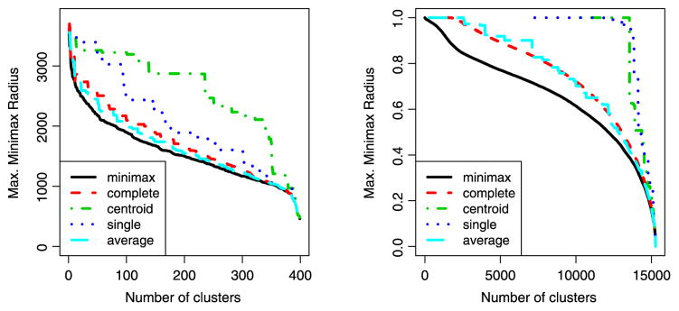
The maximum minimax radius is the farthest that any point lies from its cluster’s prototype. We see that minimax linkage hierarchical clustering does indeed do a better job of making this quantity small compared with the standard linkages. (Left) Olivetti Faces dataset. (Right) Grolier Encyclopedia dataset. The online version of this figure is in color.

6.2 Distance to Prototype versus Distance to Centroid in High Dimensions

It is well known that in high dimensions, all points of a dataset tend to lie far from all others, with none in the “center” (Bellman 1961; Hastie, Tibshirani, and Friedman 2009). In contrast, the centroid of the cluster should lie closer to most of the points. With this in mind, one would suspect that a cluster cannot be as “tightly” represented around a single element of the dataset when p ≫ n. That is, requiring each point to be within a certain distance of its cluster’s prototype likely will require a large number of clusters in this setting. We examine this phenomenon empirically using two microarray datasets, the Colon Cancer dataset, with n = 62 samples and p = 2000 genes (Alon et al. 1999), and the Prostate Cancer dataset, with n = 102 samples and p = 6033 genes (Singh et al. 2002). Because biologists in this domain use correlation as a measure of similarity between samples, we present our results in terms of correlation rather than dissimilarity as in the rest of the article.

Figure 8 compares the smallest correlation of a sample to its cluster’s prototype (using minimax linkage hierarchical clustering) to the smallest correlation of a sample to its cluster’s centroid (using complete linkage hierarchical clustering). The most relevant factor in this comparison is the prototype/centroid distinction rather than the choice of method. We find that points are less closely correlated with their prototypes than with their centroids. This can be viewed as the price to pay for the benefits in interpretability gained by using prototypes rather than centroids to describe a dataset. Surprisingly, by using prototypes instead of centroids, we do not lose very much in terms of this measure. In this situation, the curse of dimensionality is manifested as the fact that for a given minimum correlation threshold, a relatively large number of prototypes are required.

Figure 8.

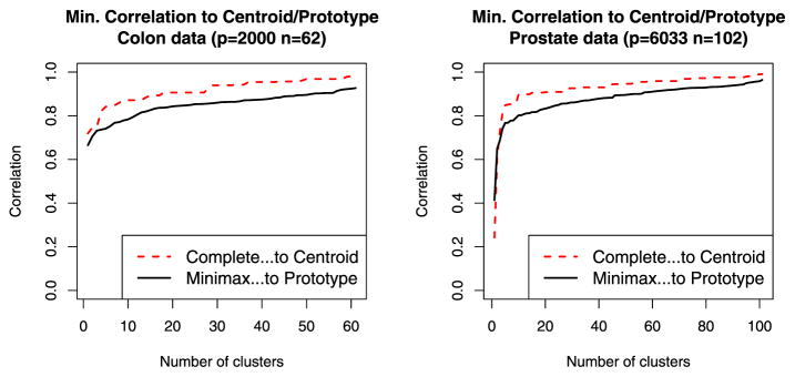
Comparison of the smallest correlation of a sample to its cluster’s prototype (using minimax linkage hierarchical clustering) to the smallest correlation of a sample to its cluster’s centroid (using complete linkage hierarchical clustering). The online version of this figure is in color.

6.3 Simulations

In this section we simulate data in which we know the underlying group structure and evaluate minimax linkage’s ability to correctly recover clusters. Given the true clustering, , of a dataset [where (x) denotes the cluster label assigned to point x], we measure the misclassification rate of a clustering by the fraction of pairs of points for which and disagree about whether they should be in the same cluster,

$$M=\frac{1}{\left(\begin{array}{c}n\\ 2\end{array}\right)}\sum _{i<j}\mid \mathbf{1}\{\mathcal{C}({\mathbf{x}}_i)=\mathcal{C}({\mathbf{x}}_j)\}-\mathbf{1}\{\mathcal{T}({\mathbf{x}}_i)=\mathcal{T}({\mathbf{x}}_j)\}\mid .$$

[This measure was used in, for example, Chipman and Tibshirani (2005), Witten and Tibshirani (2010).] In our simulations, we take to consist of three clusters, each with 100 points (i.e., n = 300) in ℝ¹⁰, sampling from N₁₀(μ₁, Σ), N₁₀(μ₂, Σ), and N₁₀(μ₃, Σ) distributions, respectively. We consider three situations:

• Spherical: μ₁ = 0, μ₂ = 2e₁ + 2e₂, μ₃ = 2e₂ + 2e₃, and Σ = I₁₀ (where e_i is the ith standard basis vector).

• Elliptical: μ₁ = 0, μ₂ = 2e₁ + 2e₂, μ₃ = 2e₂ + 2e₃, and Σ = diag(1, 1, 1, 2, 2, 1, 1, 1, 1, 1). (Note that these clusters are elongated in noise directions.)

• Outliers: Same as Spherical, but two points in cluster 2 are sampled with μ₂ = 5e₁ + 5e₂, and two points in cluster 3 are sampled with μ₃ = 5e₂ + 5e₃. By design, the outliers differ in such a way that there is little ambiguity about their proper class.

For each situation, we apply minimax, complete, average, single, and centroid linkages, with dissimilarities between the points given by both ℓ₂ and ℓ₁ distances. We let M_k denote the misclassification rate for a hierarchical clustering that has been cut to have k clusters. Thus each linkage has a corresponding sequence of values M₁, …, M_n. Table 1 reports M₃ (the misclassification rate if we were told the correct number of clusters) and M_k̂, where k̂ = arg min_k M_k. This is the best misclassification rate (over all possible cuts) that a given hierarchical clustering can possibly attain. Estimating the correct number of clusters is a difficult problem for any clustering method; thus M_k̂ is informative in that it provides a lower bound on the misclassification rate independent of the choice of where to cut. For each method and scenario, we average over 50 simulations and report standard errors in parentheses.

Table 1.

Misclassification rate (averaged over 50 simulations with standard errors given in parentheses)

		Spherical, ℓ2	Spherical, ℓ1	Elliptical, ℓ2	Elliptical, ℓ1	Outliers, ℓ2	Outliers, ℓ1
Minimax	M3	0.36 (0.01)	0.38 (0.01)	0.49 (0.00)	0.50 (0.00)	0.40 (0.01)	0.38 (0.01)
Complete	M3	0.32 (0.01)	0.37 (0.01)	0.49 (0.00)	0.50 (0.00)	0.38 (0.01)	0.38 (0.01)
Average	M3	0.64 (0.01)	0.66 (0.00)	0.54 (0.01)	0.55 (0.01)	0.65 (0.01)	0.66 (0.00)
Single	M3	0.66 (0.00)	0.66 (0.00)	0.66 (0.00)	0.66 (0.00)	0.66 (0.00)	0.66 (0.00)
Centroid	M3	0.66 (0.00)	0.66 (0.00)	0.60 (0.01)	0.60 (0.01)	0.66 (0.00)	0.66 (0.00)
Minimax	Mk̂	0.29 (0.00)	0.30 (0.00)	0.28 (0.00)	0.31 (0.00)	0.29 (0.00)	0.30 (0.00)
	k̂	11.0 (1.5)	13.2 (1.3)	25.1 (0.5)	38.8 (1.0)	10.7 (1.5)	13.2 (1.5)
Complete	Mk̂	0.28 (0.00)	0.30 (0.00)	0.29 (0.00)	0.31 (0.00)	0.28 (0.00)	0.30 (0.00)
	k̂	7.2 (0.7)	9.6 (0.8)	27.8 (0.4)	40.4 (1.0)	7.7 (0.7)	11.2 (0.9)
Average	Mk̂	0.26 (0.00)	0.27 (0.00)	0.28 (0.00)	0.30 (0.00)	0.26 (0.00)	0.28 (0.00)
	k̂	15.4 (1.1)	18.7 (1.0)	25.6 (0.4)	42.1 (0.9)	17.6 (1.2)	20.4 (1.3)
Single	Mk̂	0.33 (0.00)	0.33 (0.00)	0.25 (0.01)	0.31 (0.00)	0.33 (0.00)	0.33 (0.00)
	k̂	224.9 (3.9)	231.7 (3.3)	61.9 (2.4)	88.7 (2.0)	225.5 (4.0)	232.1 (3.3)
Centroid	Mk̂	0.33 (0.00)	0.33 (0.00)	0.28 (0.00)	0.31 (0.00)	0.33 (0.00)	0.33 (0.00)
	k̂	270.7 (2.1)	272.6 (1.7)	42.1 (1.0)	71.7 (1.3)	271.0 (2.1)	272.8 (1.7)

NOTE: M_k denotes the misclassification rate for a size-k clustering and k̂= arg min_k M_k.

The first section of the table shows that complete and minimax linkages perform much better than the other methods in all of the simulated scenarios when the true number of clusters is known (with complete linkage performing somewhat better than minimax linkage). In most cases, average, single, and centroid linkages have M₃ ≈ 0.66. Given our setting of three equalsized clusters, it is straightforward to verify that this poor misclassification rate arises when a method has two singleton clusters and one cluster with the remaining n − 2 points. Indeed, this occurs consistently for single linkage, which is known to be prone to chaining (in which many successive merges involve the addition of singletons to a large cluster). We find that in terms of M_k̂, the disparity among methods is less great (which may be expected, noting that M_k̂ ≤ M_n ≈ 0.33). In particular, we observe that average linkage attains the lowest M_k̂ values without requiring that k̂ be too large. In contrast, single linkage attains the lowest M_k̂ of any method for the elliptical-ℓ₂ case but requires more than twice the number of clusters. In summary, we find that minimax linkage performs similarly to complete linkage, which appears to be the best-performing method in our simulations.

7. ALGORITHMICS

The definition of agglomerative hierachical clustering (as described in words in Section 1) is based on the following algorithm:

Start with = {{x1}, …, {xn}} and d({xi}, {xj}) = d(xi, xj) for all i ≠ j. For l = 1, …, n − 1: Let (G1, G2) = arg d(H, K). Update = ∪ {G1 ∪ G2} \ {G1, G2}. Calculate d(G1 ∪ G2, H) for all H ∈ .

Here denotes the clustering after l steps. A straightforward implementation of the foregoing algorithm has a computational complexity of O(n³). Step 1 on iteration l requires taking the minimum over $\left(\begin{array}{c}\mid {\mathcal{C}}_l\mid \\ 2\end{array}\right)$ elements. Step 3 requires | | − 1 = n − l − 1 distance updates, so in total we do

$$\sum _{l=1}^{n-1}\left[\left(\begin{array}{c}n-l\\ 2\end{array}\right)+(n-l-1)T\right]~n^3+n^{2}T$$

operations, where T denotes the time for one distance update. The classical linkages have T = O(1), because they can all be written in terms of a Lance–Williams update (Lance and Williams 1967) as

$$d(G_1\cup G_2,H)=\alpha (G_1)d(G_1,H)+\alpha (G_2)d(G_2,H)+\beta d(G_1,G_2)+\gamma \mid d(G_1,H)-d(G_2,H)\mid ,$$ (4)

for some choice of α(·), β, γ. Minimax linkage does not fall into this class of linkages, however.

Property 6

Minimax linkage cannot be written using Lance–Williams updates.

Proof

Figure 9 shows a simple one-dimensional example that could not arise if minimax linkage followed Lance–Williams updates. The upper and lower panels show two configurations of points for which the right side of (4) is identical but the left side differs; in particular, d(G₁ ∪ G₂, H) = 9 for the upper panel, whereas d(G₁ ∪ G₂, H) = 8 for the lower panel.

Figure 9.

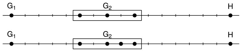
One-dimensional counterexample showing that minimax linkage cannot be written in terms of the Lance–Williams update formula.

Indeed, computing d(G₁ ∪ G₂, H) requires minimizing d_max(·, G₁ ∪ G₂ ∪ H) over |G₁ ∪ G₂| + |H| points. Thus, for iteration l, the required work for step 3 is (|G₁ ∪ G₂| + |H|) = |G₁ ∪ G₂| · | | + (n − |G₁ ∪ G₂|). If chaining occurs, we have |G₁ ∪ G₂| = l + 1, which means that in total, O(n³) work is done on step 3 as well.

Substantial improvements over this naive implementation have been made to reduce the computational complexity of the algorithms for the classical linkages (Murtagh 1983, 1984). In particular, when a linkage satisfies the reducibility property (3) and has T = O(1), the computational complexity is reduced to O(n²). We apply this technique to minimax linkage with great gains in time performance. We describe the approach in brief here; it has been presented in greater depth by Murtagh (1983).

Two points are referred to as a reciprocal nearest-neighbor (RNN) pair if each is the other’s nearest neighbor. The method exploits the property of reducible linkages in that RNN pairs are preserved when merges occur. In particular, suppose that H and K are RNNs and that G₁ and G₂ are any two other clusters. Then, by (3), if we create the merged cluster G₁ ∪ G₂, then H and K still must be RNNs. Starting with a particular point (or cluster), we may form an NN chain by repeatedly finding the next nearest neighbor. The chain cannot loop back on itself (assuming that ties do not occur); rather, a chain always ends with an RNN pair. The algorithm grows such a nearest-neighbor chain from an arbitrary point until an RNN pair is encountered, which is then removed from the chain and merged into a new cluster. We then continue extending the chain from where we left off until the next RNN pair is found. The chain continues to grow and contract in this fashion until either n − 1 merges have occurred or the chain contracts to zero length (in which case a new chain is started, again from an arbitrary object). Thus, the algorithm is as follows:

Start with = {{x1}, …, {xn}} and d({xi}, {xj}) = d(xi, xj) for all i ≠ j. The chain is empty. For l = 1, …, n − 1: If chain is empty, choose an arbitrary G ∈ ; otherwise, let G be the current end of the chain. Grow a nearest-neighbor chain from G until an RNN pair (G1, G2) is found. Update = ∪ {G1 ∪ G2} \ {G1, G2}. Calculate d(G1 ∪ G2, H) for all H ∈ . Remove G1 and G2 from the chain.

Murtagh (1984) showed that this requires O(n) nearest-neighbor searches, each of which is O(nT). Thus, in our case the algorithm is still worst case, O(n³), considering the chaining case in which T = O(n). However, we find empirically that chaining does not occur, and thus this approach is generally dramatically faster than a straightforward implementation. Figure 10 compares the time performance of our implementation of minimax hierarchical clustering with the standard Rfunction hclust. [Surprisingly, hclustdoes not appear to make use of the O(n²) nearest-neighbor chain method.] Our algorithm takes just a little more than 45 seconds to cluster n = 10,000 objects (on an Intel Xeon processor @ 3 GHz using less than 2.5 GB of RAM).

Figure 10.

Time comparison of the Rfunction hclust(complete linkage) with our implementation of minimax linkage. We find that hclust scales like n³, whereas our implementation of minimax linkage scales like n^2.4. The online version of this figure is in color.

8. DISCUSSION

We have shown that minimax linkage is an appealing alternative to the standard linkages. It has much in common with complete linkage in theoretical properties and does not have the shortcomings of centroid linkage. We have provided an efficient implementation for minimax linkage and have demonstrated in Section 5 how the minimax prototypes might be used to facilitate the interpretation of hierarchical clustering.

A common application would be to cluster genes based on a microarray dataset, in which case each label would be a gene name. A geneticist could find such a tool very useful. Although centroid linkage does associate a centroid with each node, this point is a linear combination of all objects below it, which adds little interpretative value that is not already present in the leaves. Furthermore, in situations where the data are inherently discrete (e.g., single nucleotide polymorphism data), the fractional values of the centroids would not be appropriate to the application. In Section 6.2, we investigated clustering samples (arrays), which corresponds to the task of choosing a set of prototypical samples from a set of arrays in the dataset. We found that because p ≫ n in this context, a larger number of prototypes is required here than in lower-dimensional settings. This reflects the fact that describing a dataset with only a few prototypical points from the original dataset becomes more difficult when p is large.

Inspired by minimax linkage, we can consider a more general class of prototype linkages of the form d(G, H) = r̃(G ∪ H), where r̃ is some measure of prototype-centered radius. In place of the minimax radius given in (1), we could consider replacing d_max with other measures of spread, for example, the average distance,

$$\stackrel{\sim }{r}(C)=\underset{\mathbf{x}\in C}{min}\frac{1}{\mid C\mid -1}\sum _{{\mathbf{x}}^{\prime }\in C}d(\mathbf{x},{\mathbf{x}}^{\prime }).$$

In this case, we would take the minimizing x to be the prototype for the cluster C. Unfortunately, it can be shown that the foregoing linkage has undesirable properties, such as allowing inversions.

We have implemented the nearest-neighbor chain method for minimax linkage hierarchical clustering in C, and will be releasing an R package protoclust that produces an object of class hclust compatible with standard R hierarchical clustering functions. In addition to the usual merge and height objects, the output contains an n − 1 vector of prototype indices.

References

- Alon U, Barkai N, Notterman D, Gish K, Ybarra S, Mack D, Levine A. Broad Patterns of Gene Expression Revealed by Clustering Analysis of Tumor and Normal Colon Tissues Probed by Oligonucleotide Arrays. Proceedings of the National Academy of Sciences of the USA. 1999;96:6745–6750. doi: 10.1073/pnas.96.12.6745. [DOI] [PMC free article] [PubMed] [Google Scholar]
- Ao SI, Yip K, Ng M, Cheung D, Fong P-Y, Melhado I, Sham PC. Clustag: Hierarchical Clustering and Graph Methods for Selecting Tag Snps. Bioinformatics. 2005;21(8):1735–1736. doi: 10.1093/bioinformatics/bti201. [DOI] [PubMed] [Google Scholar]
- Basalto N, Bellotti R, De Carlo F, Facchi P, Pantaleo E, Pascazio S. Hausdorff Clustering. Physical Review E. 2008;78(4):046112. doi: 10.1103/PhysRevE.78.046112. [DOI] [PubMed] [Google Scholar]
- Bellman RE. Adaptive Control Processes. Princeton, NJ: Princeton University Press; 1961. [Google Scholar]
- Chipman H, Tibshirani R. Hybrid Hierarchical Clustering With Applications to Microarray Data. Biostatistics. 2005;7:286–301. doi: 10.1093/biostatistics/kxj007. [DOI] [PubMed] [Google Scholar]
- Eisen M, Spellman P, Brown P, Botstein D. Cluster Analysis and Display of Genome-Wide Expression Patterns. Proceedings of the National Academy of Sciences of the USA. 1998;95:14863–14868. doi: 10.1073/pnas.95.25.14863. [DOI] [PMC free article] [PubMed] [Google Scholar]
- Everitt B, Landau S, Leese M. Cluster Analysis. 4. London: Arnold; 2001. [Google Scholar]
- Fisher L, Van Ness J. Admissible Clustering Procedures. Biometrika. 1971;58(1):91–104. [Google Scholar]
- Gersho A, Gray R. Vector Quantization and Signal Compression. Boston, MA: Kluwer Academic; 1992. [Google Scholar]
- Gordon AD. A Review of Hierarchical Classification. Journal of the Royal Statistical Society, Ser A. 1987;150 (2):119–137. [Google Scholar]
- Hastie T, Tibshirani R, Friedman J. Inference and Prediction. 2. New York: Springer-Verlag; 2009. The Elements of Statistical Learning; Data Mining. [Google Scholar]
- Hochbaum DS, Shmoys DB. A Best Possible Heuristic for the k-Center Problem. Mathematics of Operations Research. 1985;10(2):180–184. [Google Scholar]
- Lance GN, Williams WT. A General Theory of Classificatory Sorting Strategies: 1. Hierarchical Systems. The Computer Journal. 1967;9 (4):373–380. [Google Scholar]
- Murtagh F. A Survey of Recent Advances in Hierarchical Clustering Algorithms. The Computer Journal. 1983;26:354–359. [Google Scholar]
- Murtagh F. Complexities of Hierarchic Clustering Algorithms: State of the Art. Computational Statistics Quarterly. 1984;1:101–113. [Google Scholar]
- Singh D, Febbo PG, Ross K, Jackson DG, Manola J, Ladd C, Tamayo P, Renshaw AA, D’Amico AV, Richie JP, Lander ES, Loda M, Kantoff PW, Golub TR, Sellers WR. Gene Expression Correlates of Clinical Prostate Cancer Behavior. Cancer Cell. 2002;1:203–209. doi: 10.1016/s1535-6108(02)00030-2. [DOI] [PubMed] [Google Scholar]
- Sokal R, Mitchener C. A Statistical Method for Evaluating Systematic Relationships. The University of Kansas Science Bulletin. 1958;38:1409–1438. [Google Scholar]
- Tipping M, Schölkopf B. Artificial Intelligence and Statistics. San Francisco, CA: Morgan Kaufmann Publishers; 2001. A Kernel Approach for Vector Quantization With Guaranteed Distortion Bounds; pp. 129–134. [Google Scholar]
- Vazirani V. Approximation Algorithms. Berlin: Springer-Verlag; 2001. [Google Scholar]
- Witten D, Tibshirani R. A Framework for Feature Selection in Clustering. Journal of the American Statistical Association. 2010;105(490):713–726. doi: 10.1198/jasa.2010.tm09415. [DOI] [PMC free article] [PubMed] [Google Scholar]