A Method to Estimate Free-Living Active and Sedentary Behavior from an Accelerometer

Abstract

Methods to estimate physical activity (PA) and sedentary behavior (SB) from wearable monitors need to be validated in free-living settings.

PURPOSE

The purpose of this study was to develop and validate two novel machine-learning methods (soj-1x and soj-3x) in a free-living setting.

METHODS

Participants were directly observed in their natural environment for ten consecutive hours on three separate occasions. PA and SB estimated from soj-1x, soj-3x and a neural network previously calibrated in the laboratory (lab-nnet) were compared to direct observation.

RESULTS

Compared to the lab-nnet, soj-1x and soj-3x improved estimates of MET-hours (lab-nnet: % bias (95% CI) = 33.1 (25.9, 40.4), rMSE = 5.4 (4.6, 6.2), soj-1x: % bias = 1.9 (−2.0, 5.9), rMSE = 1.0 (0.6, 1.3), soj-3x: % bias = 3.4 (0.0, 6.7), rMSE = 1.0 (0.6, 1.5)) and minutes in different intensity categories (lab-nnet: % bias = −8.2 (sedentary), −8.2 (light) and 72.8 (MVPA), soj-1x: % bias = 8.8 (sedentary), −18.5 (light) and −1.0 (MVPA), soj-3x: % bias = 0.5 (sedentary), −0.8 (light) and −1.0 (MVPA)). Soj-1x and soj-3x also produced accurate estimates of guideline minutes and breaks from sedentary time.

CONCLUSION

Compared to the lab-nnet algorithm, soj-1x and soj-3x improved the accuracy and precision in estimating free-living MET-hours, sedentary time, and time spent in light intensity activity and MVPA. Additionally, soj-3x is superior to soj-1x in differentiating sedentary behavior from light intensity activity.

Introduction

There is a clear association between physical activity (PA) and a reduced risk for cardiovascular disease (CVD), diabetes, obesity, metabolic syndrome and some types of cancer (8). Recent research has emerged indicating sedentary behavior (SB) may also play a key role in determining an individual’s health (31). However, as outlined in the recent Physical Activity Guidelines Advisory Committee Report (PAGAC), little is known about the exact dose-response relationship between PA and specific health outcomes (8). This knowledge gap can be directly attributed to the lack of a valid method to measure behavior across the spectrum of active and sedentary behavior.

Wearable accelerometers are ideal for collecting information about free-living behavior. They can be worn for extended periods of time, impose minimal inconvenience to the participant and researcher, are relatively inexpensive and can produce detailed accounts of PA and SB that are relevant to health (e.g. estimates of energy expenditure, time in MVPA, time spent sedentary) (16). However, methods to process accelerometer output have yet to realize their potential to provide accurate estimates of energy expenditure (EE) in free-living environments (4, 16). Early work in the field used simple and multiple regressions to estimate METs (7, 11, 18, 29, 38) or kilocalories (18, 20) from accelerometer counts^·min⁻¹. Although these approaches are relatively easy to use and provide reasonable objective estimates of physical activity, their limitations have been well documented (9, 24, 35).

Recent improvements in device miniaturization, computational power and extended memory now allow data to be processed by more sophisticated machine learning algorithms. Several groups have reported success using hidden Markov models, decision trees, cross-sectional time series, multivariate adaptive regression splines and artificial neural networks (25, 33). These methods improve EE estimates and provide more detailed information about active and inactive behaviors than originally possible with traditional regression approaches (5, 12, 32, 34, 37, 41).

In a laboratory calibration study our group recently developed an artificial neural network (lab-nnet) to estimate METs from second-by-second ActiGraph^™ (ActiGraph LLC, Pensacola, Florida) accelerometer output (37). The lab-nnet improved MET estimates compared to simple regressions and has been validated on an independent sample (17). By using a single, hip-mounted accelerometer and the open-source computing language and statistics package R (39) our method preserved the simplicity and ease of use afforded by traditional regression approaches. This is particularly important to applied researchers given that most other advanced techniques use expensive analytical software (5, 34) and complex multiple accelerometer systems (3, 14, 15, 34, 40), rendering their application to free-living environments and large-scale epidemiologic studies impractical.

Although the lab-nnet performs well in laboratory settings and uses more detailed information from the acceleration signal than traditional regression approaches, it produces minute-by-minute MET estimates. This approach assumes a minute consists of only a single activity. In a laboratory this is not problematic because participants generally perform activities for a prescribed amount of time and the start and stop of activities are controlled. Prediction algorithms are then applied to bouts of homogenous activity. In free-living environments where behavior is unplanned, activities do not start and stop on the minute and several activities can be performed within the same minute (e.g. sit, stand, walk). Figure 1 illustrates the challenge of applying an algorithm developed in the laboratory to free-living data. The bottom two panels show 2-minutes and 30-seconds of free-living accelerometer output (counts^·sec⁻¹). In this example a researcher was observing the participant behavior and the recorded activities (top panel) were synchronized with the accelerometer output. When the lab-nnet is applied to these data, the five distinct activities are grouped into minute intervals (bottom panel) and METs are predicted for each minute. Preliminary observations indicate this method may produce substantial error in free-living people, and it may be necessary to first identify where activities start and stop (middle panel), and then apply the prediction algorithm to identified bouts of activity. Crouter et al (11) recognized this limitation and refined the 2006 Crouter two-regression model (10) to first identify continuous walking or running bouts before estimating METs. The refined method however, did little to improve MET estimates, which may be due to the use of static regression.

Figure 1. Measuring free-living physical activity and sedentary behavior.

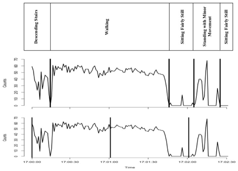
Bottom and middle panels show 2-min 30-sec of second-by-second counts from the vertical acceleration signal. Top panel shows observer-identified activities. Using the lab-nnet and simple regression approaches the five distinct activities are grouped into minute intervals (bottom panel), resulting in inaccurate MET estimates. In free-living environments it may be more appropriate to identify where bouts of activity start and stop (middle panel) and estimate METs for specific activity bouts.

We have refined our lab-nnet to be better suited for free-living applications. Our new method is called the sojourn method, and it is a hybrid machine learning technique that combines artificial neural networks with decision tree analysis. We call this method the sojourn method because an accelerometer signal from a free-living person consists of alternating periods of mostly zeros (no movement) and mostly non-zeros. The non-zeros represent sojourns of sustained activity.

The primary purpose of this study was to validate two versions of the sojourn method and our original lab-nnet in a free-living environment. The first version of the sojourn method uses second-by-second counts from the vertical axis only (soj-1x) and the second version uses second-by-second counts from the vertical, anterior-posterior and medial-lateral axes (soj-3x). We also compare results from the three machine learning approaches to three commonly used regression models (10–11, 18).

Methods

Recruitment and Eligibility

Thirteen participants (5 males, 8 females) were recruited from the surrounding community. Eligible participants were 18–60 years of age and in good physical health (no diagnosed cardiovascular, pulmonary, metabolic, joint, or chronic diseases). All participants completed a health history questionnaire and an informed consent document approved by the University of Massachusetts Institutional Review Board.

Using a standard floor stadiometer and physicians’ scale (Detecto; Webb City, MO), participant height and weight were measured to the nearest 0.25 cm and 0.1 kg, respectively. Participants also completed a short survey asking about their current physical activity status (PAS). Participants were asked to choose a number which best described their activity in a normal week. Possible responses ranged from 0 to 7 with 0 corresponding to “avoided walking or exertion (e.g. always used the elevator, drove whenever possible instead of walking)”, and 7 corresponding to “ran more than 10 miles per week or spent over 3 hours per week in comparable physical activity”.

Experimental Procedures

Direct observation served as the criterion for both the development and validation of the sojourn methods. Participants were directly observed in their free-living environment on three separate days. Each day the observation period lasted for approximately ten consecutive hours, resulting in ~30 hours of observation for each participant. During this time participants wore an ActiGraph^™ GT3X accelerometer on their right hip. The GT3X was programmed to collect data in one-second epochs from the vertical, anterior-posterior and medial-lateral axes and the normal filter mode was selected.

Criterion: Direct Observation

Observers worked in 2–4 hour shifts and a total of three different observers completed all of the observation sessions. Observers completed extensive verbal, written and video training and testing before observing participants in a free-living environment. A detailed description of the training and testing procedures is provided in Kozey Keadle et al (23). Briefly, observer training focused on strategies to avoid disrupting participant free-living behavior and methods to accurately estimate activity intensity. Upon completion of training, each observer was tested in the identification of activity type (e.g. sit, stand, walk) and intensity (e.g. 3 METs) using a ~15 minute video of free-living behavior. The video was first coded by a group of experienced observers. Study observer responses (activity type and MET value) were compared with the experienced observers’ responses using a Cohen’s kappa coefficient (κ). To be considered “in agreement” study observers needed to correctly identify both the type and intensity of the activity. There was a very high level of agreement between the study observer responses and the experienced observer responses (mean κ = 0.92). Furthermore, our direct observation method has been validated using indirect calorimetry as the criterion. DO estimates of activity intensity were highly correlated with indirect calorimetry (low intensity: intraclass correlation (ICC) = 0.99, MVPA: ICC = 0.99) and had a small bias (low intensity: percent bias = 2.1%, MVPA: percent bias = −4.9 %).

Participants were met by a trained observer in their natural environment (e.g. home, place of work, school) and observed for approximately ten consecutive hours. A hand-held personal digital assistant (PDA) (Noldus Information Technology; Netherlands) with focal sampling and duration coding was used to record participant behavior (activity type, intensity and duration). Every time behavior changed (e.g. sitting to standing) the observer recorded the new activity type and intensity in the PDA. Each entry was time stamped and the length of each behavior bout was automatically recorded in the PDA. During the ten hour observation time, subjects were allowed to have “private time” when needed. Reasons for “private time” included behaviors such as using the restroom and changing clothes. During these activities, the observer coded “private” on the PDA.

A log of the start and stop of each behavior was exported to a text file from the PDA using custom software (Noldus: Observer 9.0). These data were used to determine criterion measures of activity and inactivity variables.

Sojourn Method: Soj-1x and Soj-3x

ActiGraph^™ data were downloaded and exported to text files using ActiLife 5.0 (ActiGraph LLC, Pensacola, Florida). These data were synchronized with direct observation records downloaded from the PDA. For an observation to be included in the analyses valid DO and ActiGraph^™ data were required. Additionally, behavior coded as “private” by the observer along with the corresponding ActiGraph^™ data were eliminated from analyses. All data cleaning and processing were done using the statistics package and computing language R (39).

Method Development

Synchronized data from six randomly selected participants (18 ten-hour observations) were used to develop two versions of the sojourn method. Both sojourn methods are hybrid machine learning approaches that combine artificial neural networks with hand-built decision trees to estimate METs. The hand-built decision trees allow us to combine a priori knowledge on human behavior with the flexible non-parametric properties of the lab-nnet. This approach is well suited to estimate METs from free-living accelerometer output. The first version uses second-by-second counts from the vertical axis only (soj-1x) and the second version uses second-by-second counts from the vertical, anterior-posterior and medial-lateral axes (soj-3x).

Sojourn 1-Axis

Soj-1x uses counts^·sec⁻¹ from the vertical acceleration signal of a hip mounted ActiGraph^™ activity monitor. It requires five constants, three percentages (5%, 12% and 55%) and two time cutoffs (10 sec and 90 sec). The constants were chosen by grid search with the objective of minimizing a split sample cross-validated sum of the mean squared errors of its estimates. The step-by-step method is outlined below and illustrated in supplemental digital content (see Figure, Supplemental Digital Content 1, Sojourn-1 Axis (soj-1x) algorithm for estimating METs from free-living accelerometer data).

1. Identify Bout Intervals. To estimate bouts of activity and inactivity the soj-1x first identifies alternating intervals of various lengths where all count values are zeros (no movement of hips) or all count values are positive (movement of hips). Long intervals of zeros (≥90 sec) are identified as inactivity type 1 (sitting or lying fairly still). Long intervals of positive counts (≥10 sec) are identified as activity. Short intervals of zeros (<90 sec) and positive counts (<10 sec) are identified as “undetermined”. That temporary designation is used because there can be short intervals of positive counts during inactivity due to fidgeting or small movements, and there can be short intervals of zeros during activity due to brief bouts of standing still, these instances are temporarily called “undetermined”. Adjacent undetermined intervals are combined into longer intervals that have both zero and positive count values.

2. Determine if Undetermined Intervals are Activity or Inactivity. The next step is to identify undetermined intervals as either activity or one of four types of inactivity: 1) sitting or lying still, 2) sitting with minimal movement, 3) standing still or 4) standing with minimal movement. This is based on the percentage of non-zero counts and the duration of the interval.

   1. Inactivity type 1

      1. Non-zero counts ≤ 5%

      2. Duration ≥ 1 sec (all intervals with non-zero counts ≤ 5% are classified as inactivity type 1 regardless of duration)

   2. Inactivity type 2

      1. Non-zero counts > 5% and ≤ 12%

      2. Duration > 90 sec

   3. Inactivity type 3

      1. Non-zero counts > 5% and ≤ 12%

      2. Duration ≤ 90 sec

   4. Inactivity type 4

      1. Non-zero counts > 12% and ≤ 55%

      2. Duration ≥ 1 sec (all intervals with non-zero counts >12% and ≤ 55% are classified as inactivity type 4 regardless of duration)

   5. Activity

      1. Non-zero counts ≥ 55%

      2. Duration ≥ 1 sec (all intervals with non-zero counts ≥ 55% are classified as activity regardless of duration)

3. Estimate MET Values. The last step of soj-1x is to assign a non-physical activity MET value to inactivity types 1–4 and to estimate MET values for activity bouts. Non-physical activity MET values are based on the Compendium of Physical Activities (1) and several calibration studies (17, 22).

   1. Inactivity type 1 = 1 MET

   2. Inactivity type 2 = 1.2 METs

   3. Inactivity type 3 = 1.5 METs

   4. Inactivity type 4 = 1.7 METs

Activity MET values are estimated by applying the previously calibrated and validated lab-nnet (17, 37) to activity bouts. If the activity bout lasts for less than 120-seconds, the lab-nnet is applied to the entire bout (e.g. one MET value is estimated for the activity bout). If the bout is longer than 120-seconds, it is segmented into 40-second intervals and the lab-nnet estimates one MET value for each interval. Intervals less than 40-seconds in length are combined with the previous interval and the lab-nnet is applied to the combined interval. For example, an activity bout lasting 150 seconds is first divided into three 40-second intervals (120-seconds). The remaining 30-seconds will then be combined with the last 40-second interval, resulting in two 40-second intervals and one 70-second interval. The lab-nnet is then applied to each interval, resulting in three estimated MET values for the entire activity bout.

Sojourn 3-Axes

Soj-3x uses counts^·sec⁻¹ from the vertical, anterior-posterior and medial-lateral acceleration signals of a hip mounted ActiGraph^™ activity monitor. Soj-3x is different from soj-1x in two primary ways: 1) we identify the start and stop of activity and inactivity bout intervals differently, and 2) we apply a neural network that uses acceleration information from three axes to distinguish inactivity intervals as either sedentary (inactivity types 1 and 2) or light intensity (inactivity types 3 and 4) before we assign specific MET values. This method requires five constants, one acceleration threshold (15 counts^·sec⁻¹), one time cutoff (30 sec) and three percentages (5%, 12% and 70%). The constants were chosen by grid search with the objective minimizing a split sample cross-validated sum of the mean squared errors of its estimates. The step-by-step method is outlined below and illustrated in Figure, Supplemental Digital Content 2, Sojourn-3 Axis (soj-3x) algorithm for estimating METs from free-living accelerometer data.

1. Identify Bout Intervals. To identify the start and stop of activity and inactivity intervals, soj-3x identifies instances of rapid acceleration or deceleration. Rapid accelerations or decelerations are defined as instances where the absolute difference between adjacent counts from the second-by-second vertical acceleration signal is greater than the acceleration cutoff (≥15 counts^·sec⁻¹). In other applications, similar methods have been used to identify falls (which can be thought of as extreme posture transitions) from body worn accelerometers (33). If these intervals are less than the time cutoff (30-sec), they are combined with neighboring intervals until the combined interval is longer than the time cutoff.

2. Determine if Intervals are Activity or Inactivity. The next step is to identify intervals as either activity, or one of four types of inactivity (described in soj-1x). First, activity is distinguished from inactivity using the percentage of non-zero counts from the vertical axis. To determine inactivity types 1–4, a neural network is applied to inactivity intervals to first distinguish sitting (inactivity types 1–2) and standing (inactivity types 3–4). Sitting and standing are then further reduced to either inactivity type 1 or 2 (sitting) and inactivity type 3 or 4 (standing) based on the percentage of non-zero counts in the interval.

   1. Sitting – Determined via neural network (described below)

      1. Inactivity type 1 = Non-zero counts ≤ 5%

      2. Inactivity type 2 = Non-zero counts > 5%

   2. Standing – Determined via neural network (described below)

      1. Inactivity type 3 = Non-zero counts ≤ 12%

      2. Inactivity type 4 = Non-zero counts > 12%

   3. Activity

      • Vertical axis non-zero counts ≥ 70%

   The neural network used to distinguish sitting from standing is different than the lab-nnet used to estimate METs in soj-1x and step 3 of soj-3x. This nnet uses information about the duration of the interval and six statistical features from the vertical, anterior-posterior and medial-lateral axes, and the resultant vector magnitude of these axes:

   1. Distribution of second-by-second counts

      1. 10^th, 25^th, 50^th, 75^th and 90^th percentiles of an interval’s second-by-second counts

   2. Lag-1 autocorrelation

      • iiMeasure of relationship between adjacent counts within an interval

3. Estimate MET Values. This step is identical to the MET estimation process used in soj-1x and described above. Briefly, non-physical activity MET values are based on the Compendium of Physical Activities (1) and several calibration studies (17, 22), and the lab-nnet is used to estimate METs for activity intervals (see step 3 under soj-1x).

   Note: The purpose of soj-3x is to estimate METs. In step 2 we distinguish sitting from standing before assigning specific MET values to types of inactivity. These general intensity categories are determined from a neural network that was trained to distinguish sitting from standing activities. All sitting intervals are identified as sedentary and standing/non-sitting intervals are identified as light. Similarly, inactivity types 1–4 are assigned non-physical activity MET values based on the Compendium of Physical Activities (1) and several calibration studies (17, 22). These methods use activity type classification to improve MET estimates, an approach that is gaining popularity (6) and recently shown to improve energy expenditure estimates (2, 13).

In summary, both methods perform the following three main steps: 1) identify when bouts of activity and inactivity start and stop, 2) determine if bout intervals are activity or inactivity and 3) assign non-physical activity MET values to inactivity bouts and estimate MET values for activity bouts using the lab-nnet.

Method Validation

Data from the seven remaining participants (21 ten-hour observations) were used to validate the lab-nnet, soj-1x and soj-3x. We also compared these results to three commonly used regression models – Freedson 1998 (18), Crouter 2006 (10) and Crouter 2010 (11). All ActiGraph^™ data were processed in R and several accelerometer output variables were calculated: MET-hours, time in activity intensity categories (sedentary <1.5 METs, light 1.5–2.99 METs and moderate-to-vigorous ≥ 3 METs), minutes in bouts of activity that qualify towards meeting the physical activity guidelines (guideline minutes), the number of bouts of activity that qualify towards meeting the physical activity guidelines (guideline bouts), breaks from sitting and break rate were calculated. MET-hours describe intensity and duration as one metric (e.g. a 5 MET activity performed for 2 hours equals 10 MET-hours (5 METs × 2 hours = 10 MET-hours)) (1), and “guideline” minutes and bouts are defined as moderate-to-vigorous intensity activity that last at least ten consecutive minutes (8). Because the Freedson regression does not define a sedentary cut point, sedentary time and breaks from sedentary time were calculated using the ≤ 100 count^·min⁻¹ threshold.

Repeated measures linear mixed models were used to compare estimates to direct observation. Performance was evaluated using three statistical tools: percent bias, intraclass correlation coefficient (ICC) and root mean squared error (rMSE). Percent bias (mean difference between the estimate and criterion expressed as a percent of the criterion) provides information about the accuracy of the estimate. If the upper and lower 95% confidence intervals of the bias span 0, then we cannot detect a statistically significant difference between the estimate and the criterion at α=0.05. In this study a negative bias indicates underestimation by the prediction method, and a positive bias indicates overestimation by the prediction method. We used a two-way, mixed model ICC to test the absolute agreement of estimates and DO (icc function from R package irr) (39). An ICC closer to one indicates high agreement and an ICC closer to zero indicating low agreement. The rMSE is the square root of the mean squared error, and it provides information about the magnitude of the errors as a result of both bias and variability. It does not indicate the direction of the error (i.e. over or under-estimation).

Results

Participant characteristics (mean ± SD) are reported in Table 1. There were no differences between the development and validation groups. Results were similar for both groups, but we present results for the validation group only to show how the methods will perform on an independent sample.

Table 1.

Participant Characteristics (mean ± SD)

	Development (N=6)	Validation (N=7)	Overall (N=13)
Age (yrs.)	24.5 ± 5.9	25.0 ± 4.9	24.8 ± 5.2
Body Mass (kg)	65.0 ± 11.8	71.0 ± 14.5	68.2 ± 13.1
Height (cm)	165.3 ± 12.0	171.3 ± 9.2	168.5 ± 10.6
BMI (kg·m−2)	23.6 ± 1.3	24.0 ± 2.4	23.8 ± 1.9
PAS	6.2 ± 1.0	6.4 ± 0.5	6.4 ± 0.7

BMI=Body Mass Index, PAS=Physical Activity Status

During three DO sessions the ActiGraph^™ monitors did not record data and were therefore eliminated from analyses. This resulted in a total of 18 ten-hour validation observations from 7 validation participants. After “private time” was eliminated, mean ± SD time per observation was 9.46 ± 0.42 hours.

Table 2 shows the mean (95% CI) estimates of MET-hours and time in activity intensity categories for DO and all prediction algorithms. According to DO, participants spent on average 346.1 min (304.9–387.3) in sedentary, 161.0 min (123.4–198.6) in light and 60.4 min (46.8–73.9) in MVPA per observation. In general, soj-1x and soj-3x estimated MET-hours and moderate-to-vigorous (MVPA) intensity activity with considerably less bias (except compared to Refined Crouter MET-hours (% bias = 0.7), and produced much smaller rMSE’s compared to the lab-nnet and regression models (Table 2). Additionally, soj-3x also improved estimates of sedentary and light intensity activity. Soj-3x had an approximately 50% smaller rMSE for time in sedentary (25.5 min (15.4, 35.6)) and light (28.8 (19.5, 38.2)) intensity activity, compared to the lab-nnet (sedentary: 53.7 min (31.4, 76.0), light: 55.0 min (34.2, 75.8)), soj-1x (sedentary: 50.1 min (31.7, 68.5), light: 49.7 min (31.5, 68.0)), Freedson 1998 (sedentary: 55.7 (34.3, 77.1), light: 47.1 (28.7, 65.5)), Crouter 2006 (sedentary: 48.3 (31.1, 65.6), light: 59.2 (34.3, 84.1)) and Crouter 2010 (sedentary: 54.6 (35.1, 74.1), light: 58.0 (34.8, 81.3)). We note that because positive (overestimation) and negative (underestimation) errors cancel each other when they are averaged, an unbiased estimate does not always indicate how the model will perform for an individual.

Table 2.

Lab-nnet, Soj-1x, Soj-3x and three traditional regression models compared to direct observation (DO) (mean (95% CI))

N=18	DO	Lab-Nnet	Soj-1X	Soj-3X	Freedson	Crouter	Refined Crouter
MET-Hours	16.0 (14.8–17.3)	21.4 (20.1, 22.7)	16.4 (15.1, 17.7)	16.6 (15.0, 18.1)	14.0 (13.1, 14.9)	18.7 (17.3, 20.1)	16.0 (14.9, 17.1)
% Bias	-	33.1 (25.9, 40.4)	1.9 (−2.0, 5.9)+	3.4 (0.0, 6.7)+	−13.0 (−17.0, −8.9)	16.1 (7.8, 24.4)	0.7 (−7.1, 5.7)+
rMSE	-	5.4 (4.6, 6.2)	1.0 (0.6–1.3)	1.0 (0.6, 1.5)	2.2 (1.6, 2.7)	2.7 (1.7, 3.6)	1.4 (1.0, 1.8)
ICC	-	0.28 (−0.05, 0.16)	0.91 (0.77, 0.96)*	0.92 (0.78, 0.97)*	0.63 (−0.09, 0.89)	0.53 (−0.09, 0.83)	0.79 (0.52, 0.92)*
Sedentary Minutes	346.1 (304.9–387.3)	317.6 (283.2, 351.9)	376.4 (341.7, 411.1)	348.1 (316.5, 379.6)	391.2 (363.5, 418.9)	356.8 (325.9, 387.7)	384.0 (354.7, 413.2)
% Bias	-	−8.2 (−17.6, 1.2)+	8.8 (1.1, 16.4)	0.5 (−4.5, 5.6)+	13.7 (6.3, 21.1)	3.8 (−4.3, 11.9)+	11.6 (4.0, 19.2)
rMSE	-	53.7 (31.4, 76.0)	50.1 (31.7, 68.5)	25.5 (15.4, 35.6)	55.7 (34.3, 77.1)	48.3 (31.1, 65.6)	54.6 (35.1, 74.1)
ICC	-	0.64 (0.27, 0.85)*	0.72 (0.37, 0.89)*	0.91 (0.78, 0.97)*	0.61 (0.07, 0.85)*	0.70 (0.36, 0.87)*	0.64 (0.18, 0.86)*
Light Minutes	161.0 (123.4–198.6)	147.8 (118.2, 177.4)	131.3 (95.2, 167.4)	159.6 (128.7, 190.6)	133.3 (102.8, 163.7)	113.9 (88.3, 139.4)	111.5 (85.9, 137.1)
% Bias	-	−8.2 (−28.6, 12.2)+	−18.5 (−34.8, −2.1)+	−0.8 (−11.9, 10.3)+	−18.9 (−34.5, −3.3)	−30.9 (−49.0, −12.8)	−32.4 (−48.6, −16.1)
rMSE	-	55.0 (34.2, 75.8)	49.7 (31.5, 68.0)	28.8 (19.5, 38.2)	47.1 (28.7, 65.5)	59.2 (34.3, 84.1)	58.0 (34.8, 81.3)
ICC	-	0.54 (0.11, 0.80)*	0.71 (0.35, 0.88)*	0.89 (0.73, 0.96)*	0.68 (0.29, 0.87)*	0.47 (−0.01, 0.77)*	0.52 (−0.01, 0.81)*
MVPA Minutes	60.4 (46.8–73.9)	105.8 (89.3, 122.4)	59.8 (46.4, 73.1)	59.7 (46.8, 72.7)	43.2 (29.4, 57.0)	97.0 (81.0, 112.9)	72.2 (59.3, 5.0)
% Bias	-	72.8 (42.7, 102.9)	−1.0 (−5.5, 3.6)+	−1.0 (−7.4, 5.4)+	−28.0 (−36.3, −19.8)	58.6 (30.9, 86.3)	18.7 (4.5, 33.0)
rMSE	-	45.5 (32.2, 58.8)	4.1 (2.2, 6.0)	6.0 (3.4, 8.6)	17.0 (12.9, 21.2)	36.7 (24.6, 48.8)	14.0 (8.6, 19.3)
ICC	-	0.32 (−0.11, 0.69)	0.98 (0.95, 0.99)*	0.96 (0.90, 0.99)*	0.82 (−0.05, 0.96)*	0.41 (−0.11, 0.76)	0.82 (0.33, 0.94)*
Guideline Minutes	30.2 (15.9–44.5)	-	30.3 (15.9, 44.7)	34.0 (20.2, 47.7)	29.2 (14.6, 43.8)	45.7 (29.9, 61.7)	34.1 (18.9, 49.2)
% Bias	-	-	0.3 (−6.6, 7.1)+	12.5 (−8.0, 32.9)+	−5.0 (−13.7, 3.7)+	49.7 (32.4, 67.0)	11.0 (−2.4, 24.4)+
rMSE	-	-	1.4 (−0.1, 2.9)	7.6 (2.3, 12.9)	3.0 (0.6, 5.3)	15.1 (9.9, 20.3)	5.8 (2.4, 9.1)
ICC	-	-	0.99 (0.98, 1.00)*	0.90 (0.76, 0.96)*	0.98 (0.96, 0.99)*	0.85 (0.08, 0.96)*	0.96 (0.89, 0.99)*
Guideline Bouts	1.4 (0.8–2.0)	-	1.3 (0.7, 1.9)	1.6 (1.0, 2.2)	1.3 (0.7, 2.0)	2.5 (1.7, 3.3)	1.7 (1.0, 2.4)
% Bias	-	-	−5.0 (−28.5, 18.4)+	16.0 (−10.9, 42.9)+	−4.0 (−17.8, 9.8)+	80.0 (52.3, 107.7)	20.1 (−3.6, 43.8)+
rMSE	-	-	0.2 (0.0, 0.3)	0.4 (0.1, 0.8)	0.2 (0.0, 0.3)	1.1 (0.7, 1.5)	0.4 (0.1, 0.7)
ICC	-	-	0.95 (0.88, 0.98)*	0.81 (0.58, 0.93)*	0.96 (0.89, 0.98)*	0.68 (−0.06, 0.91)*	0.88 (0.71, 0.96)*
Breaks	29.8 (23.0–36.5)	-	39.3 (35.3, 43.3)	29.4 (23.3, 35.5)	54.4 (43.2, 65.7)	62.2 (51.5, 72.9)	56.9 (45.3, 68.4)
% Bias	-	-	32.9 (12.7, 53.1)	−1.8 (−20.4, 16.8)+	78.8 (48.7, 109.0)	106.6 (76.6,136.6)	88.7 (55.5, 121.9)
rMSE	-	-	12.1 (9.1, 15.0)	6.4 (3.4, 9.4)	24.4 (18.4, 30.5)	32.2 (26.1, 38.20)	26.9 (20.0, 33.8)
ICC	-	-	0.51 (−0.03, 0.80)*	0.79 (0.52, 0.92)*	0.46 (−0.09, 0.81)	0.33 (−0.07, 0.72)	0.40 (−0.10, 0.77)
Break-Rate	5.7 (4.0–7.4)	-	6.6 (5.5, 7.7)	−1.3 (−12.7, 10.1)	8.9 (6.7, 11.0)	11.2 (8.7, 13.8)	9.5 (7.2, 11.8)
% Bias	-	-	16.3 (1.0, 31.5)	−3.4 (−17.8, 11.1)+	0.9 (0.5, 1.3)	1.6 (0.9, 2.2)	1.1 (0.6, 1.6)
rMSE	-	-	1.6 (1.1, 2.0)	1.0 (0.6, 1.5)	0.1 (0.0, 0.1)	0.1 (0.1, 0.1)	0.1 (0.0, 0.1)
ICC	-	-	0.84 (0.58, 0.94)*	0.92 (0.80, 0.97)*	0.69 (−0.07, 0.91)	0.46 (−0.10, 0.81)	0.61 (−0.10, 0.88)

N=number of observations.

⁺Not significantly different from DO.

^*Significant correlations

All soj-1x and soj-3x estimates exhibited a significant level of agreement with DO (range: ICC = 0.51–0.99) (Table 2). In general, soj-1x and soj-3x estimates more strongly agreed with DO than the lab-nnet (range: ICC = 0.28–0.64) and regression models (range: ICC = 0.33–0.98) (Table 2). This is illustrated in Figure 2, which plots algorithm estimates against DO for each observation (N=18). Lab-nnet estimates (top panel, open squares) are more widely spread from one another than soj-1x and soj-3x, indicating the lab-nnet is less precise. Figure 2 also illustrates the higher accuracy of soj-1x (open triangles) and soj-3x (filled circles). This is evident because soj-1x and soj-3x estimates consistently fall closer to the line of identity than lab-nnet estimates. Points that fall on the line of identity indicate the estimate is identical to DO.

Figure 2.

Lab-Nnet, Soj-1x and Soj-3x estimates for each participant. Model estimates for each participant compared to direct observation. The closer the point falls to the line of identity, the closer the estimate is to direct observation. Lab-nnet: open squares, soj-1x: open triangles, soj-3x: filled circles.

Since soj-1x and soj-3x identify bouts of activity, they can provide more detailed estimates of active and sedentary behavior, including 1) minutes that qualify towards meeting the physical activity guidelines (guideline minutes), 2) the number of activity bouts that qualify towards meeting the physical activity guidelines (guideline bouts), 3) breaks from sedentary time and 4) break-rate. Both methods performed well in estimating these metrics. Table 2 and Figure 2 suggest these estimates have small biases (range: −5.0 to 32.9%), have small rMSE’s and are strongly correlated with DO (range: 0.51–0.99). The lab-nnet does not estimate activity bout duration and therefore cannot estimate this level of detail about behavior. In general, Freedson (18) and Refined Crouter (11) models performed well for estimating guideline minutes (% bias = −5.0 and 11.0, respectively), but all regression models considerably overestimated breaks from sedentary time (bias range: 78.8–106.6%) (Table 2 and Figure 3).

Figure 3.

Freedson 1998, Crouter 2006 and Crouter 2010 estimates for each participant. Model estimates for each participant compared to direct observation. The closer the point falls to the line of identity, the closer the estimate is to direct observation. Freedson 1998: open squares, Crouter 2006: open triangles, Crouter 2010: filled circles.

Discussion

In this study we presented and validated two novel methods specifically designed to estimate free-living physical activity and sedentary behavior from a single, hip-mounted accelerometer. By identifying where bouts of activity and inactivity start and stop and by predicting METs for specific bouts, soj-1x and soj-3x greatly improved the performance of the lab-nnet with direct observation as the criterion measure. Soj-1x and soj-3x also provided accurate estimates of more detailed features of behavior, including breaks from sedentary time and minutes that qualify towards meeting the physical activity guidelines (guideline minutes).

Free-living versus laboratory methods

The first step in processing sensor signals with any machine learning technique typically involves dividing the signal into small time segments called windows (33). The central difference between soj-1x, soj-3x and previous approaches is in how the signal is segmented. Laboratory methods most often use a sliding window method where the signal is divided into windows of fixed length. The lab-nnet and simple regression approaches divide the vertical acceleration signal into minute intervals and METs are estimated on a minute-by-minute basis (Figure 1). Other laboratory studies using raw acceleration have defined windows from 0.4 to 12.8 seconds (5). When sliding window methods are applied to free-living data where activities are unplanned and performed in bouts of many different durations, model performance declines considerably. This has been demonstrated previously (11) and was evident in the current study when the lab-nnet performance significantly declined compared to two previous laboratory validations (17, 37). Studies using raw acceleration and much smaller windows have reported similar observations (3, 13–15, 19, 27). Using accelerometers positioned on the sternum, wrist, thigh and lower leg, Foerester et al. (15) reported an overall 95.8% classification accuracy in the laboratory. Performance was reduced to 66.7% when the same analytic methods were applied to free-living data.

Soj-1x and soj-3x use non-fixed, activity-defined windows to segment the acceleration signal. In short, soj-1x and soj-3x use the relationship between adjacent counts from the vertical axis to identify where changes in activity may occur (see Figure Supplemental Digital Content 1 and Figure Supplemental Digital Content 2). Once the signal is segmented, the hybrid model (artificial neural network- decision tree) is applied to each window. Several methods have been proposed to identify changes in walking and gait patterns (e.g. transitioning from walking to ascending stairs, identifying heel-strike) (30, 36), but we are not aware of this approach being used to identify when bouts of activity and inactivity start and stop, or in the context of free-living physical activity measurement.

Soj-1x versus Soj-3x

In both models, information from the vertical acceleration signal is used to distinguish activity from inactivity (see Figure Supplemental Digital Content 1 and Figure Supplemental Digital Content 2). The lab-nnet is then applied to bouts of activity to estimate METs. In the current study, this approach to dealing with active bouts significantly improved estimates of time in MVPA (≥ 3 METs) (Table 2, Figure 2). Both soj-1x and soj-3x produced accurate and precise estimates, while the lab-nnet significantly overestimated time spent in MVPA. Soj-1x and soj-3x also had much smaller rMSE’s (95% CI) (4.0 min (2.1–5.9) and 7.8 min (4.1–11.8), respectively) compared to the lab-nnet (45.5 min (32.2–58.8)). Small rMSE’s suggest the model will work well for an individual – this is supported in Figure 2 where we plot individual estimates of MVPA against direct observation. Soj-1x (open diamonds) and soj-3x (filled circles) estimates consistently fall much closer to the line of identity than the lab-nnet (open squares).

Since sedentary behaviors (e.g. lying, sitting, standing still) were not included in the initial calibration of the lab-nnet and given the well-documented challenges of estimating METs for these behaviors (9, 24, 35), soj-1x and soj-3x do not use the lab-nnet to estimate METs for sedentary behaviors. Instead, soj-1x and soj-3x assign MET values from Kozey et al (22) and Ainsworth et al (1) to sedentary behaviors. To do this, soj-1x uses information from the vertical axis and soj-3x uses a simple neural network algorithm (1 hidden layer, 25 hidden units) trained on free-living data. Soj-1x did not improve estimates of time in sedentary (< 1.5 METs) and light (1.5–2.99 METs) intensity compared to the lab-nnet (Table 2, Figure 2). Conversely, soj-3x improved the estimation of sedentary time by about 50% compared to the lab-nnet, soj-1x and regression approaches (Table 2, Figure 2).

Given that soj-1x uses parameters from only the vertical acceleration signal to assign MET values to sedentary behaviors (see Figure Supplemental Digital Content 1), these results were not surprising. It is well established that the acceleration signal from the vertical axis looks very similar for sitting and standing (with minimal movement) activities (10, 23, 24). This is true for both integrated (e.g. counts^·sec⁻¹) and raw acceleration signals and in both laboratory and free-living settings (12, 14, 27, 28). Recent studies often group sedentary and light intensity behaviors into a single “low” intensity category, or estimate intensity for dynamic behaviors only (e.g. walking, running) (5, 12, 19, 40, 41). Similarly, studies aimed at identifying posture often group sitting and standing into a general “upright” category (14, 27). When this approach is not taken, the largest classification error is reported for these behaviors (5, 12). For example, during “controlled free-living” sitting and standing activities, De Vries et al. (12) reported nearly identical counts^·sec⁻¹ from the vertical axes of a hip-mounted accelerometer, resulting in standing activities being classified as sitting 78.9% of the time. More work is needed to further improve estimates of sedentary and light activities from a single hip-mounted accelerometer. The use of raw acceleration signals may provide the important detail necessary to improve these estimates even further.

Similar to the current study, Midorikawa et al (28) reported that acceleration data from three axes (vertical, anterior-posterior, medial-lateral) improved the classification of low-intensity activities compared to vertical accelerations alone. These findings and findings from other laboratory studies (5, 27) suggest information from more axes may be necessary for accurate assessment of low-intensity activities. To illustrate this, Figure 4 shows approximately 20-minutes of free-living data collected from one participant in the current study. According to direct observation, the participant is sedentary for the first third of the time, and standing in light intensity for the remaining time. Using information from the vertical signal only, soj-1x confuses light intensity with sedentary approximately half of the time. Soj-3x uses the additional information from the anterior-posterior and medial-lateral axes to correctly distinguish sedentary from light intensity. We note that if there is “not enough”, or “too much” movement in the anterior-posterior or medial-lateral planes, soj-3x will continue to confuse sedentary and light intensity activities. However, the smaller bias and rMSE for soj-3x estimates (Table 2) indicate these errors are much smaller compared to when only the vertical acceleration signal is used (soj-1x).

Figure 4.

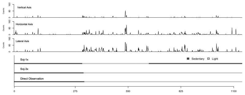
Second-by-second counts from vertical, anterior-posterior and medial-later axes (top).

Corresponding Soj-1x and Soj-3x estimates compared to direct observation (bottom).

These data illustrate an example of when the additional information from the anterior-posterior and medial-lateral axes help soj-3x correctly identify light intensity activity where soj-1x inaccurately estimates this activity as sedentary using information from the vertical axes alone.

There is currently a growing interest among physical activity epidemiologists and exercise scientists to understand the health consequences of too much sedentary time. Measurement tools and analytic approaches must continue to explore ways to accurately and precisely measure detailed characteristics sedentary behavior (i.e. total sedentary time and breaks in sedentary time). Soj-3x uses a neural network to first differentiate sitting from standing before assigning specific MET values and in the current study this approach led to a large improvement in sedentary behavior assessment compared to other methods. Using activity type classification to improve MET estimates, is an approach that has been used (6) and recently shown to improve energy expenditure estimates (2, 13)

Moving Beyond Traditional Regression

Simple linear regression was initially used to model the relationship between accelerometer counts and energy expenditure (EE) (18, 29, 38). This approach was well received by the scientific community and produces relatively accurate estimates of EE when applied to locomotion activities in a laboratory setting (10, 24, 35). The current study demonstrated the limitations of traditional regression approaches when applied in free-living settings where a range of activity types and intensities are performed. Overall performance of the Freedson regression (18) and Crouter two-regression models (10–11) were comparable to the lab-nnet. It is possible that if the acceleration signal was segmented in a similar manner to soj-1x and soj-3x, and the simple regression models were then applied to specific bouts of activity/inactivity, performance would improve. It is also important to note that although we divided our sample into a training data set and a testing data set (such that the algorithms were not trained and tested on the same observations and/or participant), soj-1x, soj-3x should be validated on an independent sample in order to verify robustness of the method and to compare performance to traditional regression methods. Nonetheless, the adaptive nature of machine learning appears to be better suited for free-living applications where a range of activity types and intensities are performed.

An important step to moving beyond traditional regression approaches is to make sophisticated data processing methods more accessible to applied researchers. The lab-nnet, soj-1x and soj-3x were developed in R, which is a free and open source software environment for statistical computing. R can be downloaded at www.r-project.org, and R programs that can be used to process second-by-second ActiGraph^™ output with soj-1x and soj-3x are on the website www.math.umass.edu/~jstauden/SojournCode.zip. The ActiGraph^™ output must be a .csv file and a wear-time log can be used to eliminate non-wear time. The programs can be used to estimate MET-hrs, time in activity intensity categories (in minutes and as a percent of wear time), guideline minutes, guideline bouts, breaks from sedentary time and break rate. There is a README file in the .zip file that explains its contents. Programming in R requires some level of expertise, but applying R functions is less of a burden to applied researchers.

Strengths and Limitations

This study has several important strengths. First, methods were validated under free-living conditions. It is well accepted that performance in the laboratory does not translate to free-living people and best practice recommendations consistently highlight the need for free-living validations (4, 16, 19, 21). Several studies have tested methods in “simulated free-living” environments where participants perform a small subset of basic ambulatory movements and postures (15, 27), but to our knowledge this is the first study to observe participants in their own natural environment and to allow participants to perform an unlimited range of activity types and intensities.

Second, participant behavior was directly observed and recorded by trained researchers for approximately ten consecutive hours. Other studies have used protocols that require participants to annotate their own behaviors (3, 25). It is unknown how accurate and reliable participant annotated data are, but intuitively this approach seems to have inherent limitations: relying on untrained participants to collect data, high degree of participant burden, inability to capture transitions between activities and inability to capture short bouts of activities. Additionally, it is unrealistic for participants to annotate their own behavior for long periods of time, thus the amount and range of data collected are limited. In this study we observed each participant, on three separate occasions, for approximately ten consecutive hours (mean hours ± SD per observation = 9.46 ± 0.42 hours). To our knowledge only one other free-living validation (19) and very few laboratory validations have compared more data to a criterion.

The third, and perhaps most important strength of this study is that the proposed methods use a single, hip mounted accelerometer (ActiGraph^™ GT3X) and an open source computing package that is on the website www.math.umass.edu/~jstauden/SojournCode.zip. The application of previous methods has been limited by complex multi-accelerometer systems and expensive analytical software (25, 26, 33). The proposed methods were successful using a relatively low sampling rate (1 Hz), information from the vertical acceleration signal only (soj-1x) and information from the vertical, anterior-posterior and medial-lateral acceleration signals (soj-3x). We anticipate that future work using much higher sampling rates (e.g. 30–100 Hz) will improve these models, but until recently monitors were not capable of collecting and storing this type of data for prolonged periods of time. Similarly, although performance improved when more information was used, the success of soj-1x is important given that earlier models of the ActiGraph^™ (e.g. 7164, GT1M) record motion in the vertical plane only and thus data collected with these monitors require vertical plane only processing techniques.

The main limitation of this study was our homogenous sample. Participants were relatively young (age = 25.0 yrs. ± 4.9 (mean ± SD)), lean (BMI = 24.0 ± 2.4) and active (PAS = 6.4 ± 0.5). It is possible the constants and thresholds used in the algorithms will need to be adjusted for use in different populations (e.g. obese, elderly). However, we anticipate future validation will demonstrate the robustness of the principles fundamental to the sojourn algorithms. Although, in this study algorithms were validated on seven participants, we do not consider sample size a limitation. Each participant was observed on three separate occasions, for approximately ten consecutive hours (mean hours ± SD per observation = 9.46 ± 0.42 hours). This resulted in approximately 12,600 minutes of direct observation synchronized with monitor output, much more data than used in other validation studies. Nonetheless, the proposed methods would benefit from future validation on larger, more diverse samples.

Finally, direct observation is a relatively novel criterion in the field of PA measurement device validation and like all measurement methods it has strengths and limitations. In direct observation, participants are observed outside of the lab for long periods of time. A strength of this approach is that we acquire specific details about behavior that cannot be captured by most other measurement methods (e.g. time in activity intensity categories and time in different postures). Direct observation also allows for an unlimited range of activity types and intensities to be performed in natural settings, which is critical for understanding how the sojourn method will perform in free-living people. However, since direct observation is used to assess features of behavior, it does not account for the individual variation in EE for a given activity. Nonetheless, as noted above, observations from our laboratory indicate that DO is an appropriate criterion for free-living validation studies.

Summary and Conclusion

Measuring and classifying human movement from accelerometer (and other) sensors is an active field that has benefited from rapid technological advancements and collaborations from experts in many fields. We are not the first to demonstrate success in using machine learning to process information from body-worn sensors (e.g. accelerometers, gyroscopes, heart-rate monitors, ambient sensors, ventilation sensors) (25, 33, 35). Very high levels of performance are generally reported, but performance consistently declines when fewer sensors are used and when methods are applied in free-living conditions (13, 19). Soj-1x and soj-3x significantly advance the field of physical activity measurement. Using a single commercially available accelerometer, open source statistical software, novel machine-learning approaches, and supervised training data collected under free-living conditions, soj-1x and soj-3x provide easy to use, accurate approaches to estimating physical activity and sedentary behavior in free-living individuals. This study also demonstrated the effectiveness of using information from the anterior-posterior and medial-lateral axes to more accurately distinguish sedentary and light intensity activity. Future validation will evaluate the sensitivity of soj-1x and soj-3x to detect change in habitual activity and future refinement will adapt these methods to also identify activity type.

Supplementary Material

1. SDC Figure 1.

Sojourn-1 Axis. Sojourn-1 Axis (soj-1x) algorithm for estimating METs from free-living accelerometer data.

2. SDC Figure 2.

Sojourn-3 Axes. Sojourn-3 Axis (soj-3x) algorithm for estimating METs from free-living accelerometer data.

References

- 1.Ainsworth BE, Haskell W, Herrmann SD, Meckes N, Bassett DR, Tudor-Locke C, Greer JL, Vezina J, Whitt-Glover MC, Leon AS. Compendium of Physical Activities: a second update of codes and MET values. Med Sci Sports Exerc. 2011;43(8):1575–81. doi: 10.1249/MSS.0b013e31821ece12. [DOI] [PubMed] [Google Scholar]
- 2.Albinali F, Intille S, Haskell W, Rosenberger M. Using wearable activity type detection to improve physical activity energy expenditure Estimation. 12th International Conference on Ubiquitous Computing; New York: ACM Press; 2010. pp. 311–320. [DOI] [PMC free article] [PubMed] [Google Scholar]
- 3.Bao L, Intille S. Pervasive. Springer-Verlag; 2004. Activity recognition from user-annotated acceleration data; pp. 1–17. [Google Scholar]
- 4.Bassett DRJ, Rowlands A, Trost SG. Calibration and validation of wearable monitors. Med Sci Sports Exerc. 2012;44(1 Suppl 1):S32–S38. doi: 10.1249/MSS.0b013e3182399cf7. [DOI] [PMC free article] [PubMed] [Google Scholar]
- 5.Bonomi AG, Goris AH, Yin B, Westerterp KR. Detection of type, duration, and intensity of physical activity using an accelerometer. Med Sci Sports Exerc. 2009;41(9):1770–77. doi: 10.1249/MSS.0b013e3181a24536. [DOI] [PubMed] [Google Scholar]
- 6.Bonomi AG, Plasqui G. Divide and conquer: assessing energy expenditure following physical activity type classification. J Appl Physiol. 2012;112(5):932. doi: 10.1152/japplphysiol.01403.2011. [DOI] [PubMed] [Google Scholar]
- 7.Brooks AG, Withers RT, Gore CJ, Vogler AJ, Plummer J, Cormack J. Measurement and prediction of METs during household activities in 35- to 45-year-old females. Eur J Appl Physiol. 2004;91(5–6):638–48. doi: 10.1007/s00421-003-1018-9. [DOI] [PubMed] [Google Scholar]
- 8.Committee PAGA; Services USDoHaH, editor. Physical Activity Guidelines Advisory Committee Report. Washington, DC: 2008. p. D-8. [Google Scholar]
- 9.Crouter SE, Churilla JR, Bassett DR., Jr Estimating energy expenditure using accelerometers. Eur J Appl Physiol. 2006;98(6):601–12. doi: 10.1007/s00421-006-0307-5. [DOI] [PubMed] [Google Scholar]
- 10.Crouter SE, Clowers K, Bassett DR., Jr A novel method for using accelerometer data to predict energy expenditure. J Appl Physiol. 2006;100(4):1324–31. doi: 10.1152/japplphysiol.00818.2005. [DOI] [PubMed] [Google Scholar]
- 11.Crouter SE, Kuffel E, Haas JD, Frongillo EA, Bassett DR., Jr Refined two-regression model for the ActiGraph accelerometer. Med Sci Sports Exerc. 2010;42(5):1029–37. doi: 10.1249/MSS.0b013e3181c37458. [DOI] [PMC free article] [PubMed] [Google Scholar]
- 12.De Vries SI, Garre FG, Engbers LH, Hildebrandt VH, Van Buuren S. Evaluation of neural networks to identify types of activity using accelerometers. Med Sci Sports Exerc. 2011;43(1):101–7. doi: 10.1249/MSS.0b013e3181e5797d. [DOI] [PubMed] [Google Scholar]
- 13.Duncan GE, Lester J, Migotsky S, Goh J, Higgins L, Borriello G. Accuracy of a novel multi-sensor board for measuring physical activity and energy expenditure. Eur J Appl Physiol. 2011;111(9):2025–32. doi: 10.1007/s00421-011-1834-2. [DOI] [PMC free article] [PubMed] [Google Scholar]
- 14.Ermes M, Parkka J, Mantyjarvi J, Korhonen I. Detection of daily activities and sports with wearable sensors in controlled and uncontrolled conditions. IEEE Trans Inf Technol Biomed. 2008;12(1):20–6. doi: 10.1109/TITB.2007.899496. [DOI] [PubMed] [Google Scholar]
- 15.Foerster FSM, Fahrenberg J. Detection of posture and motion by accelerometry: a validation study in ambulatory monitoring. Comput Hum Behav. 1999;15:571–83. [Google Scholar]
- 16.Freedson P, Bowles HR, Troiano R, Haskell W. Assessment of physical activity using wearable monitors: recommendations for monitor calibration and use in the field. Med Sci Sports Exerc. 2012;44(1 Suppl 1):S1–S4. doi: 10.1249/MSS.0b013e3182399b7e. [DOI] [PMC free article] [PubMed] [Google Scholar]
- 17.Freedson PS, Lyden K, Kozey-Keadle S, Staudenmayer J. Evaluation of artificial neural network algorithms for predicting METs and activity type from accelerometer data: Validation on an independent sample. J Appl Physiol. 2011;111(6):1804–1812. doi: 10.1152/japplphysiol.00309.2011. [DOI] [PMC free article] [PubMed] [Google Scholar]
- 18.Freedson PS, Melanson E, Sirard J. Calibration of the Computer Science and Application Inc. Accelerometer. Med Sci Sports Exerc. 1998;30(5):777–781. doi: 10.1097/00005768-199805000-00021. [DOI] [PubMed] [Google Scholar]
- 19.Gyllensten IC, Bonomi AG. Identifying types of physical activity with a single accelerometer: evaluating laboratory-trained algorithms in daily life. IEEE Trans Inf Technol Biomed. 2011;58:2656–2663. doi: 10.1109/TBME.2011.2160723. [DOI] [PubMed] [Google Scholar]
- 20.Heil DP. Predicting activity energy expenditure using the Actical activity monitor. Res Q Exerc Sports. 2006;77(1):64–80. doi: 10.1080/02701367.2006.10599333. [DOI] [PubMed] [Google Scholar]
- 21.Intille SS, Lester J, Sallis JF, Duncan G. New horizons in sensor development. Med Sci Sports Exerc. 2012;44(1 Suppl 1):S24–S31. doi: 10.1249/MSS.0b013e3182399c7d. [DOI] [PMC free article] [PubMed] [Google Scholar]
- 22.Kozey SL, Lyden K, Howe CA, Staudenmayer JW, Freedson PS. Accelerometer output and MET values of common physical activities. Med Sci Sports Exerc. 2010;42(9):1776–84. doi: 10.1249/MSS.0b013e3181d479f2. [DOI] [PMC free article] [PubMed] [Google Scholar]
- 23.Kozey Keadle S, Libertine A, Lyden K, Staudenmayer J, Freedson P. Validation of wearable monitors for assessing sedentary behavior. Med Sci Sports Exerc. 2011;43(8):1561–67. doi: 10.1249/MSS.0b013e31820ce174. [DOI] [PubMed] [Google Scholar]
- 24.Lyden K, Kozey SL, Staudenmeyer JW, Freedson PS. A comprehensive evaluation of commonly used accelerometer energy expenditure and MET prediction equations. Eur J Appl Physiol. 2011;111(2):187–201. doi: 10.1007/s00421-010-1639-8. [DOI] [PMC free article] [PubMed] [Google Scholar]
- 25.Mannini A, Sabatini AM. Machine learning methods for classifying human physical activity from on-body accelerometers. Sensors (Basel) 2010;10:1154–75. doi: 10.3390/s100201154. [DOI] [PMC free article] [PubMed] [Google Scholar]
- 26.Mathie MJ, Coster AC, Lovell NH, Celler BG. Accelerometry: providing an integrated, practical method for long-term, ambulatory monitoring of human movement. Physio Meas. 2004;25(2):R1–R20. doi: 10.1088/0967-3334/25/2/r01. [DOI] [PubMed] [Google Scholar]
- 27.Mathie MJ, Celler BG, Lovell NH, Coster ACF. Classification of basic daily movements using a triaxial accelerometer. Med Biol Eng Comput. 2004;42(5):679–87. doi: 10.1007/BF02347551. [DOI] [PubMed] [Google Scholar]
- 28.Midorikawa T, Tanaka S, Kaneko K, Koizumi K, Ishikawa-Takata K, Futami J, Tabata I. Evaluation of low intensity physical activity by triaxial accelerometry. Obesity (Silver Spring) 2007;25(12):3031–38. doi: 10.1038/oby.2007.361. [DOI] [PubMed] [Google Scholar]
- 29.Montoye HJ, Washburn R, Servais S, Ertl A, Webster JG, Nagle FJ. Estimation of energy expenditure by a portable accelerometer. Med Sci Sports Exerc. 1983;15(5):403–7. [PubMed] [Google Scholar]
- 30.Nyan MN, Tay FE, Seah KH, Sitoh YY. Classification of gait patterns in the time frequency domain. J Biomech. 2006;39(14):2647–56. doi: 10.1016/j.jbiomech.2005.08.014. [DOI] [PubMed] [Google Scholar]
- 31.Owen N, Sparling PB, Healy GN, Dunstan DW, Matthews CE. Sedentary behavior: emerging evidence for a new health risk. Mayo Clin Proc. 2010;85(12):1138–41. doi: 10.4065/mcp.2010.0444. [DOI] [PMC free article] [PubMed] [Google Scholar]
- 32.Pober DM, Staudenmayer J, Raphael C, Freedson PS. Development of novel techniques to classify physical activity mode using accelerometers. Med Sci Sports Exerc. 2006;38(9):1626–34. doi: 10.1249/01.mss.0000227542.43669.45. [DOI] [PubMed] [Google Scholar]
- 33.Preece SJ, Goulermas JY, Kenney LP, Howard D, Meijer K, Crompton R. Activity identification using body-mounted sensors--a review of classification techniques. Physio Meas. 2009;30(4):R1–33. doi: 10.1088/0967-3334/30/4/R01. [DOI] [PubMed] [Google Scholar]
- 34.Rothney MP, Neumann M, Beziat A, Chen KY. An artificial neural network model of energy expenditure using nonintegrated acceleration signals. J Appl Physiol. 2007;103(4):1419–27. doi: 10.1152/japplphysiol.00429.2007. [DOI] [PubMed] [Google Scholar]
- 35.Rothney MP, Schaefer EV, Neumann MM, Choi L, Chen KY. Validity of physical activity intensity predictions by ActiGraph, Actical, and RT3 accelerometers. Obesity (Silver Spring) 2008;16(8):1946–52. doi: 10.1038/oby.2008.279. [DOI] [PMC free article] [PubMed] [Google Scholar]
- 36.Sekine M, Tamura T, Fujimoto T, Togawa T, Fukui Y. Descrimination of walking patterns using wavelet-based fractal analysis. IEEE Trans Neural Syst Rehabil Eng. 2002;10(3):188–96. doi: 10.1109/TNSRE.2002.802879. [DOI] [PubMed] [Google Scholar]
- 37.Staudenmayer J, Pober D, Crouter S, Bassett D, Freedson P. An artificial neural network to estimate physical activity energy expenditure and identify physical activity type from an accelerometer. J Appl Physiol. 2009;107(4):1300–7. doi: 10.1152/japplphysiol.00465.2009. [DOI] [PMC free article] [PubMed] [Google Scholar]
- 38.Swartz AM, Strath SJ, Bassett DR, Jr, O’Brien WL, King GA, Ainsworth BE. Estimation of energy expenditure using CSA accelerometers at hip and wrist sites. Med Sci Sports Exerc. 2000;32:S450–6. doi: 10.1097/00005768-200009001-00003. [DOI] [PubMed] [Google Scholar]
- 39.Team RDC. R: A Language and Environment for Statistical Computing. 2008 http://www.R-project.org.
- 40.Zhang K, Werner P, Sun M, Pi-Sunyer FX, Boozer CN. Measurement of human daily physical activity. Obesity Research. 2003;11(1):33–40. doi: 10.1038/oby.2003.7. [DOI] [PubMed] [Google Scholar]
- 41.Zhang S, Rowlands AV, Murray P, Hurst T. Physical activity classification using the GENEA wrist worn accelerometer. Med Sci Sports Exerc. 2012;44(4):742–8. doi: 10.1249/MSS.0b013e31823bf95c. [DOI] [PubMed] [Google Scholar]
Associated Data
This section collects any data citations, data availability statements, or supplementary materials included in this article.
Supplementary Materials