A mathematical model of subpopulation kinetics for the deconvolution of leukaemia heterogeneity

Abstract

Acute myeloid leukaemia is characterized by marked inter- and intra-patient heterogeneity, the identification of which is critical for the design of personalized treatments. Heterogeneity of leukaemic cells is determined by mutations which ultimately affect the cell cycle. We have developed and validated a biologically relevant, mathematical model of the cell cycle based on unique cell-cycle signatures, defined by duration of cell-cycle phases and cyclin profiles as determined by flow cytometry, for three leukaemia cell lines. The model was discretized for the different phases in their respective progress variables (cyclins and DNA), resulting in a set of time-dependent ordinary differential equations. Cell-cycle phase distribution and cyclin concentration profiles were validated against population chase experiments. Heterogeneity was simulated in culture by combining the three cell lines in a blinded experimental set-up. Based on individual kinetics, the model was capable of identifying and quantifying cellular heterogeneity. When supplying the initial conditions only, the model predicted future cell population dynamics and estimated the previous heterogeneous composition of cells. Identification of heterogeneous leukaemia clones at diagnosis and post-treatment using such a mathematical platform has the potential to predict multiple future outcomes in response to induction and consolidation chemotherapy as well as relapse kinetics.

1. Introduction

Leukaemia heterogeneity develops as a result of compound genetic and micro-environmental modifications and is reflected by increased cell proliferation, block of differentiation pathways and reduction of apoptotic signals [1,2]. Cooperative effects of several mutations, as well as their order of appearance, result in cell subpopulations that acquire unique traits [3,4]. The resulting disease- and patient-specific heterogeneity is one of the main sources of variation in treatment response [1,5]. In acute myeloid leukaemia (AML), current gold-standard treatment depends on the use of cell-cycle-specific (CCS) chemotherapy. Delivery of truly personalized chemotherapy remains a challenge as most patients relapse due to clonal resistance or the emergence of more aggressive leukaemic subclones as a result of the initial chemotherapy used to treat the disease [5,6].

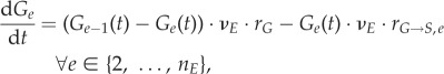
We have previously shown that assessment of proliferation kinetics and cell-cycle times in AML may provide optimized chemotherapy protocols in order to improve tumour cell kill yet minimize toxicity for the patient [7,8]. Defining the changes that occur in the cell cycle is central to these optimized treatment protocols since many chemotherapeutic drugs are cell-cycle phase-specific and heterogeneity of patient responses may be broadly defined in terms of cell-cycle phase distributions and timings [9]. The four phases of the cell cycle (G1, S, G2 and M) are governed by the periodic fluctuation in the concentration of cyclins (figure 1), a set of proteins that bind to cyclin-dependent kinases (CDKs), which are present in non-limiting concentrations [10]. Given favourable conditions, cells exit G0 and enter G1 in response to increasing cyclin D concentration. Cyclin E is produced during G1 and peaks at the transition to S phase, when it binds primarily to CDK-2, activating DNA duplication mechanisms. G2 starts when DNA synthesis is complete, and is reflected by increased cyclin B concentration, a protein that accumulates as G2 tasks are completed [11]. Once cyclin B threshold concentration is reached, it binds to CDK-1 resulting in the transition to mitosis (M). AML patients can have discrepant phase durations [9] and characteristically overexpressed/unscheduled cyclin patterns [12,13]. Together, cyclin fluctuation patterns and cell-cycle times can serve as a unique signature to define patient-specific disease characteristics mathematically, which is essential to the design of personalized treatments.

Figure 1.

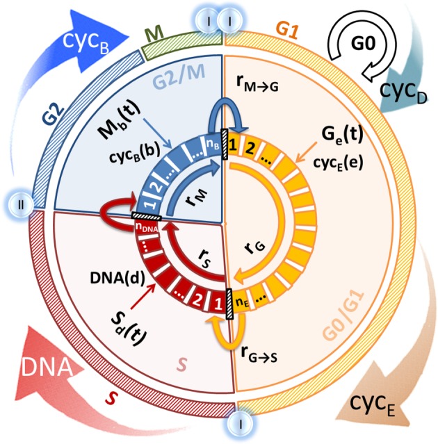
The cell cycle. Outer circles represent biological events (succession of phases and phase-specific cell-cycle protein expression); inner ‘pie’ circles summarize model simplifications and the discretization strategy based on state variable level. State variables are chosen according to relevance to their phase: cyclin E for G0/G1, DNA for S and cyclin B for G2/M. Bins in each phase indicate discrete state variable levels: C_E(e), DNA(d) and C_B(b) correspond to the state variable levels of bin number e, d and b, while cell numbers in each bin are represented by G_e(t), S_d(t) and M_b(t) in G0/G1, S and G2/M, respectively. Transition rates ( for G0/G1 and for G2/M) account for the likelihood of cells moving to the next phase and growth rates (r_G, r_S and r_M) reflect progress within the phase. (Online version in colour.)

Prior work has modelled cell-cycle phase compartments using ordinary differential equations [14]; these models quantify changes in cell number in each phase as a function of time and capture macroscopic responses of cell populations. A more detailed analysis of the system requires a description of the cell-cycle phase distribution and experimental validation of the intra-phase kinetics. A first approach could be to consider the system from the point of view of a single cell as it moves within and between phases as a function of time (discrete cells, continuous phase progression); however, this definition would be computationally expensive, unnecessary and experimentally infeasible given the need to obtain data for and model millions of cells [15]. A more efficient and tangible approach is to observe the passage of cells in time at a specific point within the phase through a population function (continuous cells, continuous phase progression). Such a model is dependent on time, but also on a state variable that distributes each phase into a continuum of populations, known as a population balance model (PBM) [16]. Solving PBMs explicitly is practically impossible in most cases; the complex task of state variable space discretization is often required. PBMs are relevant to the cell cycle in that they enable tracking of the movement of cells inside each phase through the increase in the state variable and interpret the transition between phases as the summation of exiting populations from different parts of the phase. Typically, PBMs of the cell cycle consist of three stages, namely an aggregated G0/G1 phase, S phase and an aggregated G2/M phase [17]. Traditionally, properties such as cell age, size or volume have been used as state variables. Age-based PBMs cannot be directly validated as age is not a biological property; it can be used as a mathematical artefact theoretically correlating phase coordinate to phase time; however, perturbations in the transition state cannot be explained by time alone [18]. Size- and volume-based PBMs have perhaps more relevant qualitative biologically meaningful state variables; high variability in the experimental data renders validation of these models extremely difficult requiring the estimation of the necessary parameters [19]. Finally, whereas DNA content is a very good state variable choice for S phase, where it is synthesized and can be measured, it bears no relevance to the progress of cells in other phases. Consequently, traditional PBMs cannot inform experiments with regards to the expected state variable level (as it is either a ‘virtual’ state variable or very difficult to measure); only models that specifically predict cellular properties (for a single cell) explicitly quantify these levels, but at the expense of macroscopic growth [20,21]. Hence, there is a need for cell-cycle PBMs that can be seamlessly validated experimentally and for explicit models of cell-cycle checkpoints which can incorporate growth kinetic behaviour.

Herein, we have developed a mathematical model of the cell cycle using a PBM that captures kinetics at both levels: micro (intracellular protein concentration) and macro (cell growth). The model is then used to predict heterogeneous proliferation kinetics, such as the ones presented by three leukaemic cell lines (K-562, MEC-1, MOLT-4) with very disparate origins (AML, chronic lymphocytic leukaemia and acute lymphocytic leukaemia, respectively), given a reduced set of experimental parameters.

2. Results

2.1. Development of a multi-stage population balance model based on cyclin concentration

The model is composed of three compartments according to DNA content: G (DNA content of 1), S (increasing DNA content 1–2) and M (DNA content of 2), similar to other models available [17,18]. The novelty resides in the fact that cyclin E and cyclin B are used as state variables (defined as C_E and C_B in the model) for G0/G1 and G2/M, respectively, as these are the phases where their concentration actively increases linked to phase progression. DNA content (defined as DNA in the model) is used as in previous models [19] for the representation of progress in S phase. Each of the three phases is modelled by a PBM equation (equations (2.1)–(2.3); refer to electronic supplementary material, table S2, for variable definitions), and these equations are linked by the transfer of cells from phase to phase (figure 1) [22,23]:

2.1

2.2

2.3

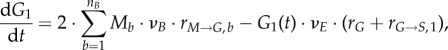
where  represents the number of cells in G0/G1 at time t that have a cyclin content C_E; similarly, and represent the number of cells in S and G2/M that have a DNA content DNA and a cyclin B content C_B, respectively, at time t. r_M→G(C_B) and r_G→S(C_E) represent the transition rates from G2/M to G0/G1 and from G0/G1 to S, respectively (both dependent on the particular phase state variable). Biologically, growth rates account for the speed at which the accumulation or production of cyclin/DNA occurs in a cell in the relevant phases. Mathematically, growth rates represent how quickly cells progress through the phase. Phase durations (T_G, T_S and T_M) are defined as the average time a cell spends in a phase. Cyclin minima represent the baseline expression at the start of the phase ( and for G0/G1 and G2/M) while cyclin thresholds ( and ) account for the average cyclin level at which cells move to the next phase. A constant cyclin E production rate (r_G) is used for G1 (equation (2.4)) [24]. DNA production (r_S) is approximated as a lineal function (equation (2.5)) based on normalized results [25]. Constant cyclin B production (r_M) occurs during G2 with a concentration plateau at transition [26]; since transition occurs rapidly, we assume a constant cyclin B production throughout G2 (equation (2.6)).

2.4

2.5

2.6

A cell in G0/G1 or G2/M can either move to the next phase or move to the next cyclin level. Biologically, the higher the cyclin concentration the more likely it is for the cell to transition. Mathematically, the transition probability (Γ(C_E) and Γ(C_B)) accounts for the likelihood of a cell at a particular position in the phase moving to the next phase, which is explicitly calculated as the ratio between transition happening (r_G→S or r_M→G) and all of transition and growth happening (r_G→S + r_G or r_M→G + r_M):

2.7

and

2.8

A recent study of different transition rate functions in cell-cycle PBMs has indicated that the particular function used had little impact on the ability of the model to fit the experimental data [27]. We assumed a normal cumulative distribution function for the transition probabilities Γ(C_E) and Γ(C_B) (see §1 in the electronic supplementary material).

The boundary conditions address the discontinuities between phases, where cells from a different phase enter a new phase. Since cells transitioning to S or to G0/G1 arrive with different cyclin concentrations from G0/G1 (equation (2.9)) or G2/M (equation (2.10)), respectively, the total number of cells is calculated by taking the integral of the transition term over all cyclin levels. For G0/G1, incoming cells are doubled to account for cell division; for S phase, all the cells with a doubled DNA content are considered to transition to the start of G2 (equation (2.11)):

2.9

2.10

2.11

Two assumptions were made: (i) the G0/G1 phase is aggregated: leukaemic cell lines are highly proliferative and therefore only a small percentage of cells with DNA content 1 will actually be quiescent (figure 2) and (ii) the G2/M phase is aggregated: the duration of the M phase is short enough compared with that of G2, such that it does not affect significantly the overall cell-cycle progress [28].

Figure 2.

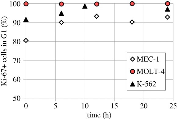
Evolution of the percentage of Ki-67 positive cells among G0/G1 cells over time (control cells) as determined by flow cytometry. Ki-67 is a protein expressed by cells out of quiescence; G0 cells are thus identified by their lack of Ki-67 expression. In the experiments performed with EdU, control cultures were monitored for Ki-67 levels to validate the assumption that only a small percentage of the cells is quiescent at any time. Indeed, Ki-67 was expressed by at least 90% of the cells overall, with the exception of MEC-1 at time 0 h which was found to be 80% (this is believed to be an effect of the washing steps stress and not a ubiquitous condition). (Online version in colour.)

Given the complexity of the equations (partial differential and integral terms), discretization of the state variable space is required. Phase domains start at (G0/G1), 1 (S) and (G2/M), and are truncated at (G0/G1), 2 (S) and (G2/M). Compartments are subdivided into n_i bins ∀ i ∈ {E; D; B}; each of the bins representing a range of state variable levels which correlates to the bin number according to the following equations:

2.12

2.13

2.14

Each bin corresponds to state variable levels that span: 1/ν_E (G0/G1 phase), 1/ν_D (S phase) and 1/ν_B (G2/M phase). The state variable levels for each bin become:

2.15

2.16

2.17

In the discrete form, equations (2.7) and (2.8) become and The model now considers n_i subpopulations ∀ i ∈ {E; D; B} corresponding to each state variable level in the compartment (figure 1), which are defined as a vector of length n_i. Following discretization of cyclins and DNA via a fully stable upwind scheme [29,30], the model equations are simplified into n_i ODEs per compartment as follows:

2.18

2.19

2.20

The discretized counterpart of (equation (2.1)) is (G_e−1(t) − G_e(t)) · ν_E · r_G (equation (2.18)); the transition term 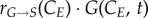corresponds to in the discretized form; change with time is converted from 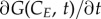to dG_e/dt. In addition, the boundary conditions become:

2.21

2.22

2.23

2.2. Experimental validation of the population balance model

EdU (5-ethynyl-2′-deoxyuridine) is a thymidine analogue that can be incorporated in the DNA of cells during S phase [9]. Cells undergoing DNA duplication are effectively labelled but not G0/G1 or G2/M cells, resulting in two separate populations that can later be tracked by flow cytometry. This provides a suitable method to generate cell-cycle ‘movies’ from which cell-cycle times can be extracted. EdU exposure does not significantly affect cell proliferation so long as the uptake is short and in low concentrations [31]. Regardless, only information from the unlabelled population was utilized. Subsequent phase deconvolution can be performed by DNA staining and the concentration of cyclins E and B is monitored by simultaneous antibody staining.

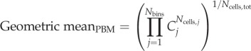
The experimental system is composed of thousands of cells, each characterized by a fluorescence intensity per channel. Global phase behaviour is obtained by normalizing the geometric mean fluorescence of individual cells [32]. A similar approach can be used in the case of the discretized model, except the system is composed of groups of cells with similar characteristics instead of single cells. The equivalence between the data analysis procedure used to aggregate flow-cytometric data and the mathematical procedure to combine the simulation data of each of the bins (refer to electronic supplementary material, figure S5, for more details) is as follows:

2.24

2.25

2.26

where i indicates the cell index and j the bin index; f_i and f_j are the normalized fluorescence of a cell and of a bin, respectively. Because equations (2.24) and (2.25) are adapted formulas for each of the systems to calculate a common variable, the resulting values are equivalent and thus comparable (electronic supplementary material, figure S5).

The transition probability function chosen implies that cells statistically never reach the maximum cyclin value in the model. It is assumed that a maximum probability of 99.99% can be achieved. Therefore, the maximum value of cyclin is theoretically obtained as the cyclin value at which 99.99% of the cells would have transitioned, which is equivalent to solving 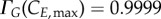and 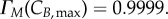A conservation analysis (detailed next) confirms this does not result in significant cell loss while providing enough flexibility for ‘outlier’ cyclin expression events to take place (electronic supplementary material, figure S1). By setting the duplication factor to one, cell numbers in the model are constant over time; the numerical solutions are tested to fulfil this property at two different levels: total cell number and final phase bins ( and ). For the total cell number, the maximum loss recorded was 1.2 × 10⁻⁵% in G phase and 2 × 10⁻⁶% in M phase (K-562). The gPROMS solver used was DASOLV with ϵ = 1 × 10⁻⁵; the cell loss is within the error of the numerical solver and therefore it can be assumed to be zero. The test for the final phase bins led to even smaller cell losses (×10⁻³⁷%). The model was additionally tested for cell conservation based on the number of discretization intervals allowed. The duplication factor was again set to 1 and the model was run for five different scenarios with n_E, n_DNA and n_B set to decreasing numbers, for a total of 1000 h. The results in terms of total cells remaining after 1000 h compared with initial cell number (represented as Total %) and percentage of cells in G0/G1 and G2/M phases exiting at the last bin are presented in electronic supplementary material, figure S1A. Discretization intervals must be reduced to very few to push the model into conservation issues. However, since we are relying on bin numbers for averaged cyclin expression, it is still important to keep a wide distribution for a good resolution in cyclin expression (otherwise situations like figure S1B, electronic supplementary material, can occur).

Because transitions are modelled according to a normal cumulative distribution, the probability of transition in the last bins of G and M ( and ) is very high (we have assumed 99.99%). When converted via equations (2.7) and (2.8), the resulting transition rates ( and ) become very high as compared to the growth rates (r_G and r_M). Therefore, the cell number that is lost through the passage to the next (non-existent) bin through growth processes is minimal, satisfying the conservation requirements:

2.27

and

2.28

In order to calculate cyclin thresholds, EdU at time 0 was considered to contain cells in late G2/M phase. and were set to the value at the peak, occurring when G_% and M_% are minimum, respectively (therefore the cells remaining are towards the end of the phase and have a cyclin content closer to the threshold). For G_%, it occurs after at least T_G − t_exposure hours, whereas for M_%, it is recorded at the very beginning (after T_M − t_exposure, which is usually close to zero because T_M tends to be in the range of EdU exposure durations). The minimum cyclin values were set as the minimum values reached in the phase of interest throughout the experiment.

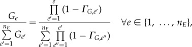
Regarding the intra-phase model initialization, two situations were encountered: even or biased cell distribution. Even phase distributions occur when cell populations are continuously coming in from the previous phase and leaving to the next phase. At steady state, the percentage of cells (with respect to the total cells in a phase) found in a bin is proportional to the complementary probability of cells transitioning from that bin (given constant intra-phase growth). A more detailed derivation can be found in §2 of the electronic supplementary material.

2.29

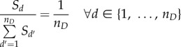2.30

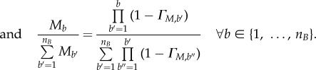2.31

Even phase distributions are used for the initial cell-cycle distribution in every phase when modelling the total population. Biased phase distributions correspond to the situation when no cells are entering a phase but cells in the phase keep progressing and exiting to the next phase, accumulating towards the end of the phase (until the phase is depleted completely). As a result of EdU exposure, the EdU⁻ population consists of G0/G1 and G2/M cells only. Specifically, G2/M cells include only those cells that were not in S phase at the start of EdU exposure. This means the EdU⁻ G2/M subpopulation is composed of cells that have been in the phase at least for the duration of the exposure, and have progressed through the phase. Therefore, the G2/M phase of the EdU⁻ population at time 0 can be modelled as a biased phase distribution. To capture this behaviour, the model was initialized for the duration of the EdU exposure and cell entrance to G2/M is blocked, resulting in the new boundary condition:

2.32

The resulting G0/G1 and G2/M intra-phase distribution at the end of the simulation of the exposure is used to initialize the model with the experimental data at time 0.

The model at this point included 283 variables and 400 parameters (measured and derived, see §6 in the electronic supplementary material). Global sensitivity analysis (GSA) identifies the parameters that have an impact on model output, by observing the change in the outputs when parameter values are varied [33]. It assesses which experimental values critically need to be determined with experimental accuracy, and which others can be estimated or kept at their nominal values for model validity. Three groups of significant parameters were identified (figure 3; see Material and methods for details): (i) and for cyclin E and B concentrations, (ii) T_G, T_S and T_M for cell-cycle phase kinetics and (iii) G_ini, S_ini and M_ini (the percentage of total cells in G1, S and G2/M at time zero) for the cell-cycle distribution. Groups (i) and (ii) were important throughout the culture, although phase times (ii) were more significant in their respective phases when a majority of cells were exiting that phase, or in their subsequent phases, when a majority of cells were entering the phase. However, group (iii) was only significant in the first few hours. Only in one of the cell lines (MEC-1) was phase kinetics affected by cyclin threshold/minimum values (maximum observed sensitivity index value for was 0.35). Conversely, cyclin concentration was only affected by cell-cycle times during the initial hours. Finally, since σ_E and σ_B were not identified as significant parameters, they were both fixed at 20% of the difference and In summary, an accurate determination of the cell-cycle times (T_G, T_S and T_M) for phase kinetics and cyclin thresholds and minima ( and ) for cyclin expression is essential to fully characterize the model.

Figure 3.

Cell-cycle phase kinetics. Comparison of experimental results (dots) to model output (lines) in cell-cycle phase per cent ((a–c) G0/G1, S, G2/M phases, respectively) or normalized cyclin E and B expression (d,e) over time. 95% confidence areas are shown according to the standard deviation of G0/G1, S and G2/M (n = 2/3). Sensitivity indexes for the most significant parameters (greater than 0.1) on each output are shown beneath. For K-562, T_G is significant in G1 at the time cells are exiting the phase (5–10 h), in S at the time they are entering the phase (5–10 h) and in G2/M when cells are entering the phase (15 h). Similarly, T_S is significant in G1 when cells are entering the phase again (15–20 h), in S when cells are exiting the phase (10–20 h) and in G2/M when cells are entering the phase (5–15 h). T_M is only significant in G2/M throughout and in the first 2–3 h for G1. For MEC-1, T_G is significant in G1 and S (to a lesser extent), T_S in S and G2/M (in G1 only at 10 h) and T_M in G2/M only. For MOLT-4, T_G is significant after 10 h in both G1 and S; T_S in S (10 h and 15), G1 (45 h) and G2/M (0–10 h); T_M in G2/M only from 5 h. For cyclin E, is the most significant parameter, followed by The same pattern is seen for cyclin B, with and (to a lesser extent) appearing significant throughout. Initial conditions (G_ini and S_ini) only appear significant in the first few hours (0–3 h) in K-562 and MEC-1. (Online version in colour.)

The cell-cycle times (T_G, T_S and T_M) were obtained by following the entrance/exit times of the EdU⁻ population (±2 h) to and from each phase for the first cycle. The initial EdU⁻ cell-cycle distribution was used to initialize and run the model. The agreement between the model and the experiments was remarkably good for all three phases in each cell line (figure 3), with the model prediction falling within the 95% confidence region for most time points. For the geometric mean of cyclin concentration, the trends and magnitudes were captured; although the experimental data were inherently noisy (due to the need for normalization steps against isotypes or other phases, which increased the number of sources for data uncertainty, and the absence of replicates), a reasonable fit was achieved. In the particular case of cyclin B concentration profile in K-562, the DNA deconvolution of the initial S-phase cell-cycle distribution places a fraction of the cells that were in the left-most section of the second DNA peak at the right-most part of S phase. Indeed, this caused a fraction of the S-phase population to enter G2/M at 2–4 h, completely shadowing the high cyclin B concentration of the remaining G2/M population at that time (figure 4a). If corrected for no cells at the end of S phase initially, the model matched the experimental data (figure 4b) in all but one point as determined by the residual sum of squares (figure 4c). Cell numbers analysed in this region are significantly lower since cells keep exiting the phase resulting in experimental data becoming less robust thus explaining the mismatch observed at 6 h.

Figure 4.

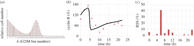
Recalculation of cyclin B trajectory when accounting for amended initial cell-cycle distribution (EdU⁻). (a) Entrance of displaced S-phase cells at 2–4 h into G2/M phase when a small, previously present population of G2/M reaches the bin where the threshold cyclin B concentration occurs. Effect due to experimental DNA deconvolution errors. (b) Geometric mean of cyclin B evolution with corrected initial conditions (no cells in the second half of S phase at time zero). Observe how the match with the model becomes closer. (c) Residual sum of squares (RSS) of the experimental and computational results of (b) over time. All but one data point fall within the experimental error region (10%). (Online version in colour.)

GSA revealed that the most significant parameters for phase kinetics were the cell-cycle times. Furthermore, the analysis showed that initial cell-cycle distribution values were not necessary for longer analyses (over 5 h). We hypothesized that co-culture conditions would have an effect on individual kinetics. A preliminary K-562/MEC-1 co-culture experiment was carried out at three set ratios: 10%, 50% and 90% MEC-1. MEC-1 kinetics was clearly slower, so its time parameters were readjusted to fit the experimental data in one of the cultures (50%), and the new model results were validated against the 10% and 90% experiments (figure 5 and electronic supplementary material, figure S2). Observe how the relative residual sum of squares is higher towards the end of the culture (figure 5c), especially in the 90% and 10% MEC-1 co-cultures, and much lower in all other time points.

Figure 5.

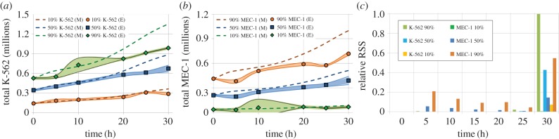
Live cell density over time. Comparison of experimental results (squares, diamonds and circles) to modelling output (dashed lines) for (a) K-562, (b) MEC-1 and (c) relative residual sum of squares (RSS). 95% confidence regions are shown according to experimental standard deviation (n = 3). Simulations performed after adjustment of kinetic parameters in co-culture. (Online version in colour.)

2.3. Forward and backward heterogeneous cell population dynamics can be predicted using the population balance model

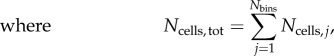
Nine different co-culture mixtures of the cell lines were prepared by operator 1 (electronic supplementary material, table S1). Operator 2, blinded to the nature of the samples, performed the analysis at time 0 and determined the initial per cent of each cell type in order to run the model. Subsequently, the rest of the samples were analysed, after which all the data were gathered and compared with model simulations. In the last three tests, the model was also evaluated for its backwards prediction capability. A pre-run plot of model predictions (see electronic supplementary material, table S4, for details of model parameters used) was used to estimate the evolution of cell line contents (figure 6a) together with the total cell number. The experimental trends for the total cell kinetics in the last three tests (T7–T9) were correctly predicted (figure 6b). Later points were overestimated; the reason for this is twofold: (i) nutrient depletion and metabolite accumulation can have a negative effect on growth which the model does not currently incorporate and (ii) MOLT-4 and MEC-1 have maximum recommended densities of 1.5–2 M cells ml⁻¹ while K-562 cannot grow at such high cell densities: T9, with a higher content of MEC-1 and MOLT-4, was correctly predicted, while for T7 and T8 (which have a majority of K-562 cells) the model overestimates the last two to three points where the cell density was over 1–1.2M cells ml⁻¹. The model accurately predicted the evolution of all cell populations for the duration of the second part of the experiment (0–30 h, figure 6c). Additionally, the contents of the original mixture (at −48 h) were found correctly in two of the three cases (figure 6a,d).

Figure 6.

Forward and backward culture evolution. (a) Ternary plot of predicted versus experimental culture evolution: lines represent model simulation of culture evolution while points denote experimental values. (b) Comparison of experimental total cell counts (dots) versus model output (dashed lines) for T7, T8 and T9. (c) Comparison of experimental cell line content (%) to model output given only the initial conditions in nine different blind tests (T1–T9) over time. (d) Backward prediction of population dynamics in T7, T8 and T9 cultures. E, experimental value; M, model prediction. Envelopes in (b) and (c) represent 95% confidence areas according to experimental standard deviation, n = 3. (Online version in colour.)

2.4. Unknown heterogeneous leukaemic populations can be deconvoluted using the population balance model platform

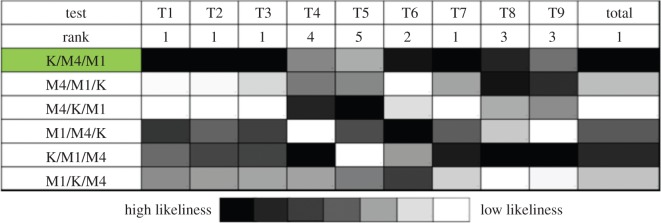
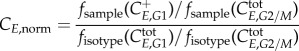
A second strategy was implemented where operator 2 pre-ran the model assigning each initial per cent to each of the cell lines (resulting in six different possible scenarios per blind experiment; electronic supplementary material, figure S3). The whole experimental panel was then revealed (unassigned to specific cell lines) and compared with the model output of each scenario in terms of Euclidian distance in a ternary plot: the lower the distance (relative to the other five scenario), the likelier to be a good match. The ranking of the scenarios likeliness given by the model for each mixture is shown in figure 7. In mixtures T1, T2, T3 and T7, the model's highest ranking candidate matched the true experimental content, while in a further three mixtures (T6, T8 and T9) the actual content was found in one of the top three candidates. Overall, the correct solution, as a sum of the Euclidian distances in all nine tests, scored lowest. Only in two cases (T4 and T5) did the model fail to identify the actual mixture as a real candidate, partly because other scenarios had extremely close values (within the experimental error margins). Of note, cells were co-cultured in non-standard conditions (cell densities and cell culture media used), challenging the ability of the PBM to work under uncertain conditions. Finally, the cell-cycle times of the three cell lines used were relatively close; primary leukaemic cells may have more disparate populations, with variation of days [9]. In this case, the differences would be largely sufficient for the model to identify and quantify heterogeneous cell populations based on cell-cycle kinetics.

Figure 7.

Ranking of scenario likeliness according to Euclidian distance between experimental data and PBM output. K/M4/M1 is the right answer in all cases, as correctly guessed by the model (K: K-562; M4: MOLT-4; M1: MEC-1). (Online version in colour.)

3. Discussion

A PBM of the cell cycle based on cyclin concentration and DNA content was developed and used to deconvolute leukaemia population kinetics. GSA established which model parameters were critically required (and which did not need to be identified) so that they were obtained experimentally for three leukaemic cell lines by following a synchronous cell population over time, after which the model was run and compared against the actual cell-cycle distribution and cyclin concentration. The agreement between the model and the experimental data was excellent, for micro (intracellular growth) as well as macro (population growth) kinetics, with most predictions falling within the 95% experimental confidence area. Additionally, residual sum of squares identified the time points where the model deviated from the experiments. The most sensitive regions included the last hours in culture (over 20 h), where cells experience exposure to significant concentration gradients in terms of nutrient depletion and metabolite accumulation (figure 5c); and regions where the number of cells analysed is not sufficient to provide an accurate representation of the phenomena occurring in culture (figure 4c). Next, the model was successfully used for two different strategies in the context of co-culture kinetics: (i) the prediction of backward and forward culture evolution given known cell line-specific cell-cycle kinetics and initial conditions and (ii) the identification of cell type and content given an unknown experimental panel.

Clonal heterogeneity of AML and competitive outgrowth of more ‘fit’ clones in a ‘Darwinian’ model render the successful treatment of this disease particularly challenging [34]. It is currently unclear which factors within a subclone or in the microenvironment make certain clones out-compete others and how this dynamic can be altered by chemotherapy schedule [9,34,35]. Recently, it has been proposed that tumour-specific cell-autonomous and non-cell-autonomous factors (e.g. cytokines) can alter growth kinetics and properties of tumours and that these qualities may be targeted to manipulate tumour growth [36]. Although there are many other properties relevant to leukaemia and the treatment of leukaemia, most if not all of these factors ultimately affect the cell cycle. Hence, this work describes a model of the cell cycle that can be combined or upgraded to capture additional phenomena such as differentiation (affecting traditional chemotherapy, but also affected by novel agents targeting specific types of haematopoietic cells) or environmental cues (metabolism, cytokines, contact inhibition, etc.). The key is capturing the most important phenomena at a sufficient level of detail in order to maintain the fidelity and relevance to the biological system. Defining which are the additional phenomena that are key in response to chemotherapy is definitely a critical step. Pharmacokinetics/pharmacodynamics (PK/PD) models capture body processes that are relevant to the drug distribution and transport to the bone marrow, as well as its effect, for example. Our model may be able to capture clonal heterogeneity which, combined with PK/PD, may lead to improved and more effective therapies.

The ability to assess both backward and forward evolution of cell clonal content using the PBM presented herein provides a quantitative tool for the estimation of population dynamics and the study of leukaemia progression in both treated and untreated patients [6,37,38]. This tool also has the potential to evaluate clonal models of leukaemogenesis [4,6,39] in order to better understand the pathogenesis of disease. In the context of CCS drug dosage and scheduling, the PBM could give a narrower window of action than what is currently used in treatment regimens, thereby limiting drug toxicity yet improving efficacy [8,7]. Drugs, such as small molecule inhibitors, currently being tested that specifically target leukaemia subclones (e.g. those expressing FLT3-ITD [40]) could be dosed and scheduled to optimize cell kill during therapy according to anticipated subclonal composition. Ultimately, balancing CCS chemotherapy with more advanced gene-targeted treatments will require detailed knowledge of subpopulation evolution, kinetics and dynamics during treatment calculated and manipulated using computational methods such as those presented herein for designer therapies. The availability of individual clone sensitivities to each drug (EC50) and the use of accurate models simulating drug distribution in the human body will be key for simulating cell death by chemotherapy. The PBM's high resolution in describing intra-phase events allows incorporating cell death not only in a phase-specific but also in a phase coordinate-specific manner (data not shown).

Genome-based methods are currently employed in order to define mutational heterogeneity in AML subclones, thereby identifying evolution of disease throughout treatment [6]. In order to optimize treatments in AML, we pursued a complementary strategy of clonal identification by using cell-cycle kinetics to effectively represent heterogeneity. Cells may acquire proliferative mutations that modify cell-cycle times through bypassing of cell-cycle controls; overexpression of p21 enables cells with DNA damage to continue to the next phase prematurely [41], while mutations in Cdc20 delay the timing of cyclin B degradation, and pRb or E2F mutations promote early entry into S phase by premature increase in the concentration of cyclin E [42]. A plethora of subpopulations, each with specific cell cycle signatures arises; the PBM can estimate cell-cycle evolution for each of them and capture overall behaviour. Since cell-cycle duration has been shown to correlate with prognosis in response to treatment [43], an a priori classification of subpopulations according to slow/intermediate/fast cell-cycle kinetics may be initially developed. A more sophisticated extrapolation for patient cell populations is currently being studied by the use of steady-state parameters [44], rather than the dynamic counterparts (used here), which could potentially be measured in the diagnostic bone marrow or peripheral blood sample at disease presentation. Technology now exists wherein patient AML mutations and subclones are identified routinely [45]. Put together with cell-cycle data (which could be done at diagnosis and throughout treatment if needed by assessment of S-phase or cyclin expression by flow cytometry), PK/PD combined models are being developed to optimize chemotherapy dose and schedule according to anticipated clonal output [8,44]. With this method, there is the potential to tailor treatments by manipulating leukaemic heterogeneity and instilling long-term control of tumour growth, limiting expansion of more pathogenic clones [36,46].

Heterogeneous cyclin production patterns originate as a result of cell-cycle mutations (e.g. cyclins D1 and E1, KIP1, INK4B and INK4A, CDK4, Rb [11]), making them leukaemia-specific. Predicting the intensity and timing of cyclin concentration increase can become critical in defining the optimal dose and schedule of current as well as novel treatment strategies [8,47]. Owing to their critical role in the control of cell-cycle progression, cyclin-blockade strategies arrest proliferation, without the risk of additional mutagenesis inherent in traditional chemotherapeutics. Specific cell-cycle drug targets, such as cyclin D and CDK1–cyclin B complexes [48,49], may be identified and tracked using the PBM platform developed herein and used to identify the best dose and schedule pre-clinically, expediting drug development trajectories.

The development of detailed models of the cell cycle that are experimentally validated is critical in the implementation of more advanced PK/PD models [50,51]. Additionally, linking a small subset of measurable variables to unique characteristics of the individual is necessary for the development of personalized treatment. The PBM we have developed paves the way in connecting both. Ultimately, the application of such a tool could inform not only optimal timing and type of personalized treatment for improved outcomes but also provide a platform for pre-clinical assessment of novel targeted therapies for leukaemia and other cancers.

4. Material and methods

4.1. Computational tools

The computational tools used for carrying out the simulations in this paper are detailed below, as well as the sensitivity analysis methods. The model was implemented on gPROMS ModelBuilder 3.5.3 and simulated on a 64-bit Windows with an Intel Core 2 Quad CPU 2.67 GHz and 4GB RAM. GSA was performed on Matlab for the discretized model by connecting gPROMS through gO:Matlab. Sobol's method [52] was used, screening the influence of 24 parameters with 20 000 intervals each on the G1–S–G2/M phase per cents, cyclin expression, % cell loss, transition rates and total cell number. The inputs were varied ±40%, built onto a matrix in Matlab^® and a call was sent sequentially via gO:Matlab^® for every set of parameter values. The outputs at 0, 1, 2, 5, 10, 15 and 20 h for each parameter were recorded and the sensitivity indexes were subsequently calculated on GUI-HDMR [53] Matlab package. The analysis was made on the model including the reinitialization period for EdU exposure (biased phase distribution).

4.2. Leukaemia cell lines

Cell lines are laboratory-adapted populations that give reproducible experimental results and require basic culture methods for their maintenance. Three leukaemia cell lines were used: K-562 (chronic myeloid leukaemia in blast crisis; has unscheduled cyclin E production and overexpressed cyclin B [54]); MEC-1 (chronic lymphoid leukaemia, which expresses CD19) and MOLT-4 (acute lymphoid leukaemia, has scheduled cyclin E and B [13]). K-562 (ATCC, MD, USA) was cultured in Isocove modified Dulbecco's medium (IMDM; Invitrogen, CA, USA) with 10% heat inactivated fetal bovine serum (FBS; Invitrogen) and 1% penicillin–streptomycin (P/S; Invitrogen). MEC-1 (DSMZ, Germany) cells were cultured in IMDM + 20% FBS + 1% P/S for 1 week, and in IMDM + 10% FBS + 1% P/S thereafter. MOLT-4 (ATCC) cells were cultured in RPMI-1640 (Invitrogen) + 10% FBS + 1% P/S. All cells lines were used at p < 20.

4.3. Labelling cells with 5-ethynyl-2′-deoxyuridine

In vitro labelling of cells with EdU is necessary to segregate the global population into two approximately synchronous populations for dynamics to be observed. The AF647 EdU kit (Invitrogen) was reconstituted and used according to manufacturer's instructions. Cells were resuspended in fresh medium and pre-cultured for 12 h in T175 flasks (Corning, NY, USA) at 300 000 cells ml⁻¹ (K-562), 400 000 cells ml⁻¹ (MEC-1) or 350 000 cells ml⁻¹ (MOLT-4). EdU (10 nM) was added (optimal concentration was determined by preliminary experiments, data not shown) and after 1 h (MEC-1) or 2 h (K-562, MOLT-4), cells were washed twice and resuspended in fresh medium for culture under standard conditions in six-well plates (Corning; 4–6 ml per well). Two cultures were exposed with a difference of 11–14 h; samples were collected every 2 h for intervals of up to 14 h consecutively and the data were merged (overlap in cell-cycle distribution values was confirmed at matching points). An unexposed culture was used as a control.

4.4. Co-culture experiments

Co-culture indicates an experimental set-up where two or more separate cell lines are physically put together in the same culture medium. In order to distinguish the populations, specific analysis methods detecting each of them individually have to be developed. K-562 and MEC-1 cells were mixed at the appropriate ratios and pre-cultured in IMDM + 10% FBS. After 48 h, they were resuspended in fresh medium at a density of 0.5 × 10⁶ cells ml⁻¹ and cultivated in six-well plates (Corning), 4 ml per well. Triplicate samples of 10⁶ cells were taken at 0, 5, 10, 20, 25 and 30 h. For the blinded experiments, operator 1 prepared unknown mixtures of K-562, MEC-1 and MOLT-4 cell lines (different cell types and ratios), which were precultured for 48 h. Samples were taken every 5–10 h for a total of 30 h. Triplicate samples were collected and split into two tests: samples to be stained for CD19 and fixed in paraformaldehyde 4% and samples to be fixed in ethanol for later detection of cyclin B concentration. In the segmentation of co-cultured samples, the percentage of MEC-1 cells was inferred from the population with CD19 expression, the MOLT-4 content from the population with high cyclin B concentration (electronic supplementary material, figure S4); K-562 was the % remaining. For samples where only K-562 and MOLT-4 were present, SSC versus DNA analyses sufficed to gate each cell type. Note that this was impossible when all three cell lines were together as SSC versus DNA of MEC-1 overlaps with both K-562 and MOLT-4 (only approximate values of per cent of each cell line could be deduced).

4.5. Flow cytometry

Flow cytometry is a technique that allows translating single cell properties (DNA content, protein expression) to fluorescence intensity by labelling them with antibodies specific to the protein or substances that bind to DNA strands and fluoresce when exposed to a laser beam of a particular wavelength. The cyclin B IgG1κ antibody kit (clone GNS-1; BD, NJ, USA) was used according to manufacturer's instructions. Anti-human cyclin E antibody (clone HE12), together with the isotype control IgG1 (clone ICIGG1) and the FITC secondary antibody to IgG were prepared as per manufacturer's protocol (all three from Abcam, UK). The V450 Ki-67 IgG1κ (clone B56, BD) antibody and V450 IgG1κ isotype control (clone MOPC-21, BD) were both diluted 4×. A propidium iodide (PI; Sigma, MO, USA) solution was prepared by dissolving 10 mg l⁻¹ PI with 100 mg l⁻¹ DNase-free RNase (Sigma) in phosphate buffered saline (PBS; Invitrogen), as previously described [51]. Triplicate samples were collected regularly for each condition (EdU: every 2 h; No EdU: every 6 h) and fixed in 70% ethanol at −20°C for a maximum of 2 days prior to acquisition. Cells were then labelled with antibodies after permeabilization in the following order: (i) exposure to EdU reagent, (ii) staining with either cyclin B or E antibodies and (iii) resuspended in PI.

For CD19 labelling in co-culture experiments, labelled or control antibody was added to each of the three replicate samples and incubated for 30 min at 4°C in the dark, fixed in paraformaldehyde at 4°C, and data were acquired within 2 days with a Guava flow-cytometer (easyCyte 8HT, Millipore, MA, USA); a Fortessa flow cytometer (LSRFortessa, BD) was used for all other data acquisition. FACSDiva software was used during acquisition of data on Fortessa, while easyCyte was used on the Guava; for all samples, 20 000 events were acquired. Data analysis, gating and geometric mean calculations were performed in FlowJo 8.7 (TreeStar Inc, OR, USA).

In order to process these data, several steps have to be performed for every sample: (i) gating out the debris on the FSC versus SSC, (ii) gating out the doublets on the PI (area) versus PI (width) signal, (iii) deconvoluting the cell-cycle distribution (Dean–Jett–Fox method) resulting in G0/G1, S (split into four equal gates at time 0 only) and G2/M gates, (iv) gating the EdU positive from the EdU negative populations (from control which was unexposed to EdU but exposed to click reaction cocktail) and (v) gating the cyclin positive from the cyclin negative populations (from isotype control exposed to EdU and reaction cocktail). From this analysis, four different populations are identified: EdU⁺ C⁺; EdU⁺ C⁻; EdU⁻ C⁺; EdU⁻ C⁻, in addition to the ungated total population. For each sample: (i) the geometric mean of the fluorescence in the C ⁺ population in the phase of interest divided by the geometric mean of the fluorescence in the total population in the phase where the cyclin expression is minimal gives the normalized sample expression, (ii) for the isotype samples, the geometric mean of the fluorescence in the phase of interest divided by the geometric mean of the fluorescence in the total population in the phase where the cyclin expression is minimal gives the baseline expression of the phase and finally (iii) the normalized values obtained in (i) are divided by the baseline values from (ii) giving the normalized cyclin expression of the phase of interest for the sample:

4.1

and

4.2

Data accessibility

The experimental data presented in the paper are provided as an Excel attachment.

Authors' contributions

M.F.G. wrote the manuscript and carried out the experiments, data processing, model development, parameter estimation, GSA and model validation. R.M. carried out the experiments and participated in the model development, as well as providing feedback throughout. D.G.M. provided the initial version of the PBM and the idea of using cyclins as state variables, as well as input in the process of adaptation for leukaemia. E.V. gave feedback on experimental results. M.K. and M.C.G. developed and provided the method for discretizing the PBM. E.N.P. gave feedback on model development and validation. N.P. reviewed the manuscript and provided advice on clinical relevance of the results presented here. A.M. reviewed the manuscript and suggested the idea of a co-culture blinded experiment for model validation. All authors gave final approval for publication.

Competing interests

We declare we have no competing interests.

Funding

This work is supported by ERC-BioBlood (340719; M.F.G., E.V.), ERC-Mobile Project (226462; E.V.), by the EU 7th Framework Programme (MULTIMOD Project FP7/2007–2013, 238013; M.F.G., D.G.M.) and by the Richard Thomas Leukaemia Research Fund. R.M. is grateful for a Royal Academy of Engineering Research Fellowship.

References

- 1.Ley TJ, et al. 2013. Genomic and epigenomic landscapes of adult de novo acute myeloid leukemia. N. Engl. J. Med. 368, 2059–2074. ( 10.1056/NEJMoa1301689) [DOI] [PMC free article] [PubMed] [Google Scholar]
- 2.Kelly LM, Gilliland DG. 2002. Genetics of myeloid leukemias. Annu. Rev. Genomics Hum. Genet. 3, 179–198. ( 10.1146/annurev.genom.3.032802.115046) [DOI] [PubMed] [Google Scholar]
- 3.Warner JK, Wang JC, Hope KJ, Jin L, Dick JE. 2004. Concepts of human leukemic development. Oncogene 23, 7164–7177. ( 10.1038/sj.onc.1207933) [DOI] [PubMed] [Google Scholar]
- 4.Klco JM, et al. 2014. Functional heterogeneity of genetically defined subclones in acute myeloid leukemia. Cancer Cell 25, 379–392. ( 10.1016/j.ccr.2014.01.031) [DOI] [PMC free article] [PubMed] [Google Scholar]
- 5.Meacham CE, Morrison SJ. 2013. Tumour heterogeneity and cancer cell plasticity. Nature 501, 328–337. ( 10.1038/nature12624) [DOI] [PMC free article] [PubMed] [Google Scholar]
- 6.Ding L, et al. 2012. Clonal evolution in relapsed acute myeloid leukaemia revealed by whole-genome sequencing. Nature 481, 506–510. ( 10.1038/nature10738) [DOI] [PMC free article] [PubMed] [Google Scholar]
- 7.Pefani E, Panoskaltsis N, Mantalaris A, Georgiadis MC, Pistikopoulos EN. 2013. Design of optimal patient-specific chemotherapy protocols for the treatment of acute myeloid leukemia (AML). Comput. Chem. Eng. 57, 187–195. ( 10.1016/j.compchemeng.2013.02.003) [DOI] [Google Scholar]
- 8.Pefani E, Panoskaltsis N, Mantalaris A, Georgiadis MC, Pistikopoulos EN. 2014. Chemotherapy drug scheduling for the induction treatment of patients with acute myeloid leukemia. IEEE Trans. Biomed. Eng. 61, 2049–2056. ( 10.1109/TBME.2014.2313226) [DOI] [PubMed] [Google Scholar]
- 9.Preisler HD, Raza A, Gopal V, Ahmad S, Bokhari J. 1995. Distribution of cell-cycle times amongst the leukemia cells within individual patients with acute myelogenous leukemia. Leuk. Res. 19, 693–698. ( 10.1016/0145-2126(95)98846-P) [DOI] [PubMed] [Google Scholar]
- 10.Pietras EM, Warr MR, Passegue E. 2011. Cell cycle regulation in hematopoietic stem cells. J. Cell Biol. 195, 709–720. ( 10.1083/jcb.201102131) [DOI] [PMC free article] [PubMed] [Google Scholar]
- 11.Malumbres M, Barbacid M. 2001. To cycle or not to cycle: a critical decision in cancer. Nat. Rev. Cancer 1, 222–231. ( 10.1038/35106065) [DOI] [PubMed] [Google Scholar]
- 12.Iida H, Towatari M, Tanimoto M, Morishita Y, Kodera Y, Saito H. 1997. Overexpression of cyclin E in acute myelogenous leukemia. Blood 90, 3707–3713. [PubMed] [Google Scholar]
- 13.Gong JP, Ardelt B, Traganos F, Darzynkiewicz Z. 1994. Unscheduled expression of cyclin-B1 and cyclin-E in several leukemic and solid tumor-cell lines. Cancer Res. 54, 4285–4288. [PubMed] [Google Scholar]
- 14.Daukste L, Basse B, Baguley BC, Wall DJN. 2012. Mathematical determination of cell population doubling times for multiple cell lines. Bull. Math. Biol. 74, 2510–2534. ( 10.1007/s11538-012-9764-7) [DOI] [PubMed] [Google Scholar]
- 15.Singhania R, Sramkoski RM, Jacobberger JW, Tyson JJ. 2011. A hybrid model of mammalian cell cycle regulation. PLoS Comput. Biol. 7, e1001077 ( 10.1371/journal.pcbi.1001077) [DOI] [PMC free article] [PubMed] [Google Scholar]
- 16.Ramkrishna D. 2000. Population balances: theory and applications to particulate systems in engineering. San Diego, CA: Academic Press. [Google Scholar]
- 17.Sidoli FR, Asprey SP, Mantalaris A. 2006. A coupled single cell-population-balance model for mammalian cell cultures. Ind. Eng. Chem. Res. 45, 5801–5811. ( 10.1021/ie0511581) [DOI] [Google Scholar]
- 18.Sherer E, Hannemann RE, Rundell A, Ramkrishna D. 2006. Analysis of resonance chemotherapy in leukemia treatment via multi-staged population balance models. J. Theor. Biol. 240, 648–661. ( 10.1016/j.jtbi.2005.11.017) [DOI] [PubMed] [Google Scholar]
- 19.Liu YH, Bi JX, Zeng AP, Yuan JQ. 2007. A population balance model describing the cell cycle dynamics of myeloma cell cultivation. Biotechnol. Prog. 23, 1198–1209. ( 10.1021/bp070152z) [DOI] [PubMed] [Google Scholar]
- 20.Tyson JJ. 1991. Modeling the cell-division cycle—Cdc2 and cyclin interactions. Proc. Natl Acad. Sci. USA 88, 7328–7332. ( 10.1073/pnas.88.16.7328) [DOI] [PMC free article] [PubMed] [Google Scholar]
- 21.Weis MC, Avva J, Jacobberger JW, Sreenath SN. 2014. A data-driven, mathematical model of mammalian cell cycle regulation. PLoS ONE 9, e97130 ( 10.1371/journal.pone.0097130) [DOI] [PMC free article] [PubMed] [Google Scholar]
- 22.García Münzer DG, Kostoglou M, Georgiadis MC, Pistikopoulos EN, Mantalaris A. 2014. A cyclin distributed cell cycle model in GS-NS0. Comput. Aided Process Eng. 33, 19–24. ( 10.1016/B978-0-444-63456-6.50004-1) [DOI] [PMC free article] [PubMed] [Google Scholar]
- 23.García Münzer DG, Kostoglou M, Georgiadis MC, Pistikopoulos EN, Mantalaris A. 2015. Cyclin and DNA distributed cell cycle model for GS-NS0 cells. PLoS Comput. Biol. 11, e1004062 ( 10.1371/journal.pcbi.1004062) [DOI] [PMC free article] [PubMed] [Google Scholar]
- 24.Ohtsubo M, Theodoras AM, Schumacher J, Roberts JM, Pagano M. 1995. Human cyclin-E, a nuclear protein essential for the G(1)-to-S phase-transition. Mol. Cell. Biol. 15, 2612–2624. [DOI] [PMC free article] [PubMed] [Google Scholar]
- 25.Avva J, Weis MC, Sramkoski RM, Sreenath N, Jacobberger JW. 2012. Dynamic expression profiles from static cytometry data: component fitting and conversion to relative, ‘same scale’ values. PLoS ONE 7, e38275 ( 10.1371/journal.pone.0038275) [DOI] [PMC free article] [PubMed] [Google Scholar]
- 26.Kang Q, Pomerening JR. 2012. Punctuated cyclin synthesis drives early embryonic cell cycle oscillations. Mol. Biol. Cell 23, 284–296. ( 10.1091/mbc.E11-09-0768) [DOI] [PMC free article] [PubMed] [Google Scholar]
- 27.Chaffey GS, Lloyd DJB, Skeldon AC, Kirkby NF. 2014. The effect of the G(1)–S transition checkpoint on an age structured cell cycle model. PLoS ONE 9, e83477 ( 10.1371/journal.pone.0083477) [DOI] [PMC free article] [PubMed] [Google Scholar]
- 28.Morgan D. 2007. The cell cycle: principles of control. London, UK: New Science Press Ltd. [Google Scholar]
- 29.Kostoglou A, Karabelas AJ. 1995. Evaluation of numerical methods for simulating an evolving particle size distribution in growth processes. Chem. Eng. Commun. 136, 177–199. ( 10.1080/00986449508936360) [DOI] [Google Scholar]
- 30.Lapidus L, Pinder GF. 1982. Numerical solution of partial differential equations in science and engineering. New York, NY: Wiley-Interscience. [Google Scholar]
- 31.Cappella P, Gasparri F, Pulici M, Moll J. 2008. A novel method based on click chemistry, which overcomes limitations of cell cycle analysis by classical determination of BrdU incorporation, allowing multiplex antibody staining. Cytometry A 73A, 626–636. ( 10.1002/cyto.a.20582) [DOI] [PubMed] [Google Scholar]
- 32.Münzer DGG, Kostoglou M, Georgiadis MC, Pistikopoulos EN, Mantalaris A. 2013. Developing a cyclin blueprint as a tool for mapping the cell cycle in GS-NSO. Biochem. Eng. J. 81, 97–107. ( 10.1016/j.bej.2013.10.008) [DOI] [Google Scholar]
- 33.Kiparissides A, Koutinas M, Kontoravdi C, Mantalaris A, Pistikopoulos EN. 2011. ‘Closing the loop’ in biological systems modeling—from the in silico to the in vitro. Automatica 47, 1147–1155. ( 10.1016/j.automatica.2011.01.013) [DOI] [Google Scholar]
- 34.Greaves M, Maley CC. 2012. Clonal evolution in cancer. Nature 481, 306–313. ( 10.1038/nature10762) [DOI] [PMC free article] [PubMed] [Google Scholar]
- 35.Stiehl T, Baran N, Ho AD, Marciniak-Czochra A. 2014. Clonal selection and therapy resistance in acute leukaemias: mathematical modelling explains different proliferation patterns at diagnosis and relapse. J. R. Soc. Interface 11, 20140079 ( 10.1098/rsif.2014.0079) [DOI] [PMC free article] [PubMed] [Google Scholar]
- 36.Marusyk A, Tabassum DP, Altrock PM, Almendro V, Michor F, Polyak K. 2014. Non-cell-autonomous driving of tumour growth supports sub-clonal heterogeneity. Nature 514, 54–58. ( 10.1038/nature13556) [DOI] [PMC free article] [PubMed] [Google Scholar]
- 37.Walter RB, et al. 2014. Heterogeneity of clonal expansion and maturation-linked mutation acquisition in hematopoietic progenitors in human acute myeloid leukemia. Leukemia 28, 1969–1977. ( 10.1038/leu.2014.107) [DOI] [PMC free article] [PubMed] [Google Scholar]
- 38.Wiseman DH, Greystoke BF, Somervaille TC. 2014. The variety of leukemic stem cells in myeloid malignancy. Oncogene 33, 3091–3098. ( 10.1038/onc.2013.269) [DOI] [PubMed] [Google Scholar]
- 39.Shackleton M, Quintana E, Fearon ER, Morrison SJ. 2009. Heterogeneity in cancer: cancer stem cells versus clonal evolution. Cell 138, 822–829. ( 10.1016/j.cell.2009.08.017) [DOI] [PubMed] [Google Scholar]
- 40.Serve H, et al. 2013. Sorafenib in combination with intensive chemotherapy in elderly patients with acute myeloid leukemia: results from a randomized, placebo-controlled trial. J. Clin. Oncol. 31, 3110–3118. ( 10.1200/JCO.2012.46.4990) [DOI] [PubMed] [Google Scholar]
- 41.Viale A, et al. 2009. Cell-cycle restriction limits DNA damage and maintains self-renewal of leukaemia stem cells. Nature 457, 51–56. ( 10.1038/nature07618) [DOI] [PubMed] [Google Scholar]
- 42.Schnerch D, et al. 2012. Cell cycle control in acute myeloid leukemia. Am. J. Cancer Res. 2, 508–528. [PMC free article] [PubMed] [Google Scholar]
- 43.Raza A, et al. 1990. Direct relationship between remission duration in acute myeloid-leukemia and cell-cycle kinetics—a Leukemia Intergroup Study. Blood 76, 2191–2197. [PubMed] [Google Scholar]
- 44.Fuentes-Garí M, et al. 2015. Cell cycle model selection for leukemia and its impact on chemotherapy outcomes. In 12th Int. Symp. on Process Systems Engineering and 25th European Symp. on Computer Aided Process Engineering (eds Gernaey KV, Huusom JK, Gani R.). Computer Aided Chemical Engineering, vol. 37 Amsterdam, The Netherlands: Elsevier. [Google Scholar]
- 45.Buccisano F, Maurillo L, Del Principe MI, Del Poeta G, Sconocchia G, Lo-Coco F, Arcese W, Amadori S, Venditti A. 2012. Prognostic and therapeutic implications of minimal residual disease detection in acute myeloid leukemia. Blood 119, 332–341. ( 10.1182/blood-2011-08-363291) [DOI] [PubMed] [Google Scholar]
- 46.Zhao BY, Hemann MT, Lauffenburger DA. 2014. Intratumor heterogeneity alters most effective drugs in designed combinations. Proc. Natl Acad. Sci. USA 111, 10 773–10 778. ( 10.1073/pnas.1323934111) [DOI] [PMC free article] [PubMed] [Google Scholar]
- 47.Sawai CM, et al. 2012. Therapeutic targeting of the cyclin D3:CDK4/6 complex in T cell leukemia. Cancer Cell 22, 452–465. ( 10.1016/j.ccr.2012.09.016) [DOI] [PMC free article] [PubMed] [Google Scholar]
- 48.Lapenna S, Giordano A. 2009. Cell cycle kinases as therapeutic targets for cancer. Nat. Rev. Drug Discov. 8, 547–566. ( 10.1038/nrd2907) [DOI] [PubMed] [Google Scholar]
- 49.Musgrove EA, Caldon CE, Barraclough J, Stone A, Sutherland RL. 2011. Cyclin D as a therapeutic target in cancer. Nat. Rev. Cancer 11, 558–572. ( 10.1038/nrc3090) [DOI] [PubMed] [Google Scholar]
- 50.Velliou E, Fuentes-Garí M, Misener R, Pefani E, Rende M, Panoskaltsis N, Mantalaris A, Pistikopoulos EN. 2014. A framework for the design, modeling and optimization of biomedical systems. In Proc. 8th Int. Conf. on Foundations of Computer-Aided Process Design (eds Eden MR, Siirola JD, Towler G.). Computer Aided Chemical Engineering, vol. 34, pp. 225–236. Amsterdam, The Netherlands: Elsevier; ( 10.1016/B978-0-444-63433-7.50023-7) [DOI] [Google Scholar]
- 51.Fuentes-Garí M, Velliou E, Misener R, Pefani E, Rende M, Panoskaltsis N, Mantalaris A, Pistikopoulos EN. In press. A systematic framework for the design, modeling and optimization of personalized healthcare: making and healing blood. Comput. Chem. Eng. ( 10.1016/j.compchemeng.2015.03.008) [DOI] [Google Scholar]
- 52.Sobol IM. 2001. Global sensitivity indices for nonlinear mathematical models and their Monte Carlo estimates. Math. Comput. Simul. 55, 271–280. ( 10.1016/S0378-4754(00)00270-6) [DOI] [Google Scholar]
- 53.Ziehn T, Tomlin AS. 2009. GUI-HDMR—a software tool for global sensitivity analysis of complex models. Environ. Model. Softw. 24, 775–785. ( 10.1016/j.envsoft.2008.12.002) [DOI] [Google Scholar]
- 54.Viallard JF, Lacombe F, Dupouy M, Ferry H, Belloc F, Reiffers J. 1999. Flow cytometry study of human cyclin B1 and cyclin E expression in leukemic cell lines: cell cycle kinetics and cell localization. Exp. Cell Res. 247, 208–219. ( 10.1006/excr.1998.4352) [DOI] [PubMed] [Google Scholar]
Associated Data
This section collects any data citations, data availability statements, or supplementary materials included in this article.
Supplementary Materials
Data Availability Statement