EBSeq-HMM: a Bayesian approach for identifying gene-expression changes in ordered RNA-seq experiments

Abstract

Motivation: With improvements in next-generation sequencing technologies and reductions in price, ordered RNA-seq experiments are becoming common. Of primary interest in these experiments is identifying genes that are changing over time or space, for example, and then characterizing the specific expression changes. A number of robust statistical methods are available to identify genes showing differential expression among multiple conditions, but most assume conditions are exchangeable and thereby sacrifice power and precision when applied to ordered data.

Results: We propose an empirical Bayes mixture modeling approach called EBSeq-HMM. In EBSeq-HMM, an auto-regressive hidden Markov model is implemented to accommodate dependence in gene expression across ordered conditions. As demonstrated in simulation and case studies, the output proves useful in identifying differentially expressed genes and in specifying gene-specific expression paths. EBSeq-HMM may also be used for inference regarding isoform expression.

Availability and implementation: An R package containing examples and sample datasets is available at Bioconductor.

Contact: kendzior@biostat.wisc.edu

Supplementary information: Supplementary data are available at Bioinformatics online.

1 Introduction

With improvements in next-generation sequencing technologies and reductions in price, ordered RNA-seq experiments are becoming common. Of primary interest in these experiments is characterizing how genes are changing over some factor with ordered levels (for example, ordered in time, in space, along a gradient, etc). For simplicity, we refer to any ordered RNA-seq experiment as a time-course experiment, noting that other similar designs may be analyzed within this framework; and we restrict attention to time-course data collected within a single biological condition.

In a time-course RNA-seq experiment, an investigator may be interested in genes that are monotonically increasing or decreasing, that increase initially then decrease, that increase initially then remain unchanged and so on. We refer to these types of changes in expression hereinafter as expression paths, and we consider three broad types: (i) constant paths: expression remains unchanged, or equally expressed (EE), over all time points; (ii) sporadic paths: expression shows some change between at least one pair of time points, but remains unchanged between at least one other pair and (iii) dynamic paths: expression changes continuously. With respect to the examples listed earlier, the first few (expression is monotonically increasing, monotonically decreasing, increasing then decreasing) are instances of dynamic paths. The last (increase initially then remain unchanged) is an example of a sporadic path.

A number of robust statistical methods are available for identifying differentially expressed (DE) genes [EBSeq (Leng et al., 2013), DESeq2 (Love et al., 2014), edgeR (Robinson et al., 2010), voom (Law et al., 2014), baySeq (Hardcastle and Kelly, 2010), Cuffdiff2 (Trapnell et al., 2012)] as well as isoforms [EBSeq, rSeqDiff (Shi and Jiang, 2013), Cuffdiff2, BitSeq (Glaus et al., 2012)] in a static RNA-seq experiment; and most of these methods accommodate time-course experiments by considering time as a factor with multiple, unordered, levels (Supplementary Section S7 provides details). The statistical tests employed are designed to identify a gene as DE if it shows a change at least one time point; and, consequently, non-constant genes are detected collectively. Multiple steps of subsequent analyses are required if an investigator wants to distinguish sporadic paths from dynamic ones, to classify genes into distinct paths and to assess the associated classification uncertainty—for example, perform model fitting multiple times with different design matrices and then adjust for multiple testing. In addition, as these approaches were not designed specifically for time-course experiments, they do not accommodate dependence over time and consequently sacrifice power if applied in this setting.

These same issues were addressed in the context of microarray time-course experiments, and a number of methods are available for analyzing (Conesa et al., 2006; Filkov et al., 2002; Ma et al., 2009; Yuan and Kendziorski, 2006) and clustering (Ernst et al., 2005; Luan and Li, 2003) time-course microarray data. These methods are not directly applicable to RNA-seq studies since they do not accommodate count data, the unequal variabilities in measurements or the dependence of isoforms within genes. To address this, the approach developed by Conesa et al. (2006), maSigPro, originally developed for microarray time-course analysis, was recently extended to accommodate ordered RNA-seq count data (Nueda et al., 2014). Like DESeq2 and edgeR, maSigPro-GLM is based on a negative binomial (NB) generalized linear model (GLM); but unlike previous approaches, maSigPro-GLM defines gene-specific expected expression by a time-dependent polynomial to accommodate dependence over time. Once significant genes are selected, a second regression is conducted for each gene to identify the time points at which it shows expression differences. Clustering algorithms are then applied to the resulting regression coefficients and/or expression values to identify groups of genes with similar expression profiles. Although useful the two step procedure makes it challenging to determine appropriate thresholds for false discovery rate (FDR) control, and suggested thresholds are conservative in many settings (Nueda et al., 2014). In addition, identified gene groups are subject to limitations inherent in clustering algorithms; namely, the number of groups as well as group membership are determined by user-defined cutoffs, there is no probabilistic information associated with a given gene’s membership within a group, and it is not clear how to classify gene groups into expression paths.

To address these considerations, we have developed an empirical Bayes auto-regressive hidden Markov model (HMM) based approach called EBSeq-HMM. The model extends our previous work, EBSeq, for identifying DE genes and isoforms across two or more biological conditions (Leng et al., 2013). As detailed in Methods, an auto-regressive process describes changes in expression over time, and a hidden Markov component is used to accommodate dependence. EBSeq-HMM allows users to identify genes with non-constant expression over multiple ordered conditions, and simultaneously classify them into expression paths. Results from a simulation study, detailed in Section 3.1, suggest that EBSeq-HMM has increased power over competing approaches for identifying genes following non-constant paths, especially for those genes showing subtle yet consistent changes over time. EBSeq-HMM also provides improved accuracy in classifying genes into expression paths. Similar results are demonstrated in a case study of the adult mouse limb presented in Section 3.2.

2 Methods

2.1 EBSeq-HMM: an empirical Bayes auto-regressive Hidden Markov model

EBSeq-HMM requires estimates of gene or isoform expression collected over three or more ordered levels of a factor. The general model is presented for gene-level analysis; the isoform-level model is discussed in Section 2.3. To simplify the presentation, we refer to ordered levels as time points denoted by $t=1,2,\dots ,T$, noting that the method directly accommodates other ordered data structures (e.g. ordered in space, along a gradient, etc.).

Let $X_t$ be a $G\times N_t$ matrix of expression values for G genes in N_t samples at time t. The full set of observed expression values is then denoted by $X=\left(X_1,X_2,\dots ,X_T\right)$. With a slight abuse of notation, let $X_g$ denote one row of this matrix containing data for gene g over time; X_gtn denotes expression values for gene g at time t in sample n. Of interest are changes in the latent mean expression levels for gene g: ${\mu }_{g1},{\mu }_{g2},\dots ,{\mu }_{gT}$. We allow for three possibilities, or states, to describe such changes: Up, Down, EE. If ${\mu }_{t-1}<{\mu }_t$, we define state $S^{\Delta t}$ as Up; if ${\mu }_{t-1}>{\mu }_t,S^{\Delta t}$ is Down and ${\mu }_{t-1}={\mu }_t$ defines $S^{\Delta t}$ as EE. The main goals in an ordered RNA-seq experiment—identifying genes that change over time, and specifying each genes’ expression path—can be restated as questions about these underlying states. In short, for each gene g and each transition between t−1 and t, we would like to estimate the probability of each state. A gene is said to follow a non-constant path if at least one state is not EE. We would also like to estimate the most likely expression path, which is given by the configuration of expression states over time ($S_g^{\Delta 2},S_g^{\Delta 3},\dots ,S_g^{\Delta T}$), noting that the most likely configuration of states need not equal the collection of states that define $S_g^{\Delta t}$ marginally at each t (an example is provided in Section 3.1).

To make inference regarding these states, we propose a model for the set of expression measurements taken on a gene g. We make the common and well-supported assumption that gene expression in an RNA-seq experiment is well described by a NB distribution (Anders and Huber, 2010; Hardcastle and Kelly, 2010; Love et al., 2014; Nueda et al., 2014; Robinson et al., 2010; Trapnell et al., 2012). Were we to consider time t in isolation, this implies $X_{gtn}|r_{gt},q_{gt}\sim NB(r_{gt},q_{gt})$ where the NB distribution may be parameterized such that ${\mu }_{gt}=r_{gt}(1-q_{gt})/q_{gt}$. For simplicity of notation, we assume equal library sizes. Details on adjustments for unequal library sizes are given in Supplementary Section S2.

Because our interest here is in quantifying changes in $X_{gt}$ over time, we assume expression at time t depends on that at t−1 through parameters r and q. Specifically, $\left(X_{gtn}|r_{g,t-1},q_{g,t-1},S_g^{\Delta t}=s\right)\sim \text{NB}(r_{g,t-1}{\xi }_g^s,q_{g,t-1})$ where ${\xi }_g^s=c$ if s is Up; ${\xi }_g^s=1/c$ if s is Down and ${\xi }_g^s=1$ if s is EE. The data dependent parameter c specifies the expected change associated with each state. For example, if c = 2, then $S_g^{\Delta t}$ = Up refers to a 2-fold increase in expression between t−1 and t. Although c may be defined by a user, we suggest estimation by maximum likelihood (see the next section). We further model fluctuations in μ_gt by defining a prior distribution for $q_{gt}:\left(q_{gt}|\alpha ,\beta ,X_{g,t-1}=x_{g,t-1}\right)\sim Beta(\alpha +N_{t-1}{r}_{g,t-1},\beta +{\displaystyle {\sum }_j{x}_{g,t-1,j}})$ for all g and t > 1. Given this set-up, when t > 1, the marginal predictive conditional distribution describing expression (or emissions) for each state is Beta-NB: $\left(X_{gtn}|X_{g,t-1}=x_{g,t-1},S_g^{\Delta t},\Theta \right)\sim \text{Beta–NB}(\alpha +N_{t-1}{r}_{g,t-1},\beta +{\displaystyle {\sum }_j{x}_{g,t-1,j}},{\xi }_g^s{r}_{g,t-1})$ where $\Theta =\left[\alpha ,\beta ,r_{g,t-1},{\xi }_g^s\right]$. The expected mean is then defined as ${\xi }_g^s{r}_{g,t-1}(\beta +{\displaystyle {\sum }_j{x}_{g,t-1,j}})/(\alpha +N_{t-1}{r}_{g,t-1})$ (Teerapabolarn, 2008). When t = 1, the prior distribution for $q_{g1}$ is defined as $\left(q_{g1}|\alpha ,\beta \right)\sim Beta(\alpha ,\beta )$ for all g, and the marginal predictive distribution is $\left(X_{g1n}|\Theta \right)\sim \text{Beta–NB\hspace{0.17em}}(\alpha ,\beta ,r_{g,1})$.

For genes with dynamic paths, each state $S_g^{\Delta t}$ is dependent on the prior state $S_g^{\Delta t-1}$ since these genes represent continuous changes over time. To accommodate this dependence, we assume that the state process is described by a Markov chain. The constant and sporadic genes do not show continuous changes over time, and consequently we assume that states are independent, although we note that dependence among expression levels is still accommodated via the auto-regressive component.

In summary, the time-course $X_g$ for a dynamic gene is governed by two interrelated probabilistic mechanisms: the conditional distribution (emissions model) at each time and the process describing the evolution of states over time. Initially, we assume that the observed expression vector can be characterized by the Beta-NB model described earlier and that the state process can be described by a Markov chain. Were it the case that dependence among measurements is fully captured by the state process, the proposed model would be a standard HMM. However, this last assumption does not hold, given that X_t for dynamic genes depends not only on the state $S^{\Delta t}$ but also on $X_{t-1}$ through $r_{t-1}$. Consequently, the model for dynamic genes is given by a Markov-switching auto-regressive model, as in Hamilton (1989) and Ailliot and Monbet (2012) (Fig. 1). For constant and sporadic genes, we assume the same emissions model, but do not assume the state process is Markov. Taken together, since we do not know the expression path type a priori, the model for the full set of expression measurements is a two-component mixture over the sporadic/constant and dynamic genes.

Fig. 1.

(a) An auto-regressive hidden Markov component models dynamic paths. (b) An auto-regressive non-hidden Markov component models constant and sporadic paths

2.2 Parameter estimation

In the emissions distributions, the unknown parameters (r’s, α and β) are estimated using the method of moments (r’s are estimated within time point while α and β are estimated using all samples); c is estimated via maximum likelihood. Recall that EBSeq-HMM assumes a mixture model with a Markov component m1 and a non-Markov component m2. We assume equal prior probabilities of being in each mixture component.

In Markov chain m1, the Baum-Welch algorithm is used to estimate initial ${\pi }_j=P(S_g^{{\Delta }_2}=j|m1)$ and state transition probabilities $a_{dj}^{t,t+1}=P(S_g^{{\Delta }_{t+1}}=j|S_g^{{\Delta }_t}=d,m1)$ for $t\ge 2$. Here, we assume a non-homogeneous Markov chain for the hidden states so $a_{dj}^{t,t+1}$’s are different for different t’s. Denote the vector of initial probabilities and the state transition matrices estimated from the last step as ${\displaystyle \stackrel{\sim }{\pi }},{\displaystyle \stackrel{\sim }{A}}$. Given parameter estimates ${\displaystyle \stackrel{\sim }{\pi }},{\displaystyle \stackrel{\sim }{A}}$, define $z_g^{m1}=P(M_g=m1|X_g,{\displaystyle \stackrel{\sim }{\pi }},{\displaystyle \stackrel{\sim }{A}})$ and $b_j(X_{gt})=P(X_{gt}|S_g^{{\Delta }_t}=j,X_{g,t-1}=x_{g,t-1})$. The forward and backward steps of the Baum-Welch algorithm are then defined as follows:

$$\begin{array}{c}{\alpha }_{g,j}(t)=[{\displaystyle \sum _d{\alpha }_{g,d}}(t-1){{\displaystyle \stackrel{\sim }{a}}}_{dj}^{t-1,t}]b_j(X_{g,t})\\ \propto P(X_{g1},\dots ,X_{gt},S_g^{{\Delta }_t}=j|m1)\\ {\beta }_{g,j}(t)={\displaystyle \sum _d[{\beta }_{g,d}(t+1)b_d(X_{g,t+1}){{\displaystyle \stackrel{\sim }{a}}}_{jd}^{t,t+1}]}\\ \propto P(X_{g,t+1},\dots ,X_{gT}|X_{gt},S_g^{{\Delta }_t}=j,m1)\end{array}$$

The initial and state transition probabilities are updated by:

$$\begin{array}{c}{a}_{D,J}^{t,t+1}=\frac{{\displaystyle \sum _{g}P}(S_g^{{\Delta }_t}=D,S_g^{{\Delta }_{t+1}}=J,M_g=m1|X_g,{\displaystyle \stackrel{\sim }{\pi }},{\displaystyle \stackrel{\sim }{A}})}{{\displaystyle \sum _g{\displaystyle \sum _{j}P}}(S_g^{{\Delta }_t}=D,S_g^{{\Delta }_{t+1}}=j,M_g=m1|X_g,{\displaystyle \stackrel{\sim }{\pi }},{\displaystyle \stackrel{\sim }{A}})}\\ =\frac{{\displaystyle \sum _g{\alpha }_{g,D}}(t){{\displaystyle \stackrel{\sim }{a}}}_{D,J}^{t,t+1}{b}_{g,J}(X_{g,t+1}){\beta }_{g,J}(t+1)z_g^{m1}}{{\displaystyle \sum _g{\displaystyle \sum _j{\alpha }_{g,D}}}(t){{\displaystyle \stackrel{\sim }{a}}}_{D,j}^{t,t+1}{b}_{g,j}(X_{g,t+1}){\beta }_{g,j}(t+1)z_g^{m1}}\\ {\pi }_J=\frac{{\displaystyle \sum _{g}P}(S_g^{{\Delta }_2}=J,M_g=m1|X_g,{\displaystyle \stackrel{\sim }{\pi }})}{{\displaystyle \sum _g{\displaystyle \sum _{j}P}}(S_g^{{\Delta }_2}=j,M_g=m1|X_g,{\displaystyle \stackrel{\sim }{\pi }})}\\ =\frac{{\displaystyle \sum _g{\alpha }_{g,J}}(2){\beta }_{g,J}(2)z_g^{m1}}{{\displaystyle \sum _g{\displaystyle \sum _j{\alpha }_{g,j}}}(2){\beta }_{g,j}(2)z_g^{m1}}\end{array}$$

Parameters are estimated by fixing expected fold-change (FC) c at 1.2. The process is then repeated for c in (1.4, 1.6, … , 3); and the parameter set with maximum likelihood is used in the final model.

2.3 Inference at the isoform level

The model detailed in the previous section applies to gene counts. To apply the approach to isoforms, the uncertainty inherent in isoform expression estimation should be accommodated. In short, estimating expression at the gene-level is a relatively easy task in RNA-seq as all reads mapping to a gene’s constituent exons may be used. The same holds true for estimating expression for an isoform unique to its parent gene. However, for genes with multiple isoforms, the problem is more challenging as reads mapping to overlapping exons (exons present in more than one isoform) must be allocated to isoforms in a way that is consistent with their expression. Consequently, there is increased uncertainty (on average) in expression estimates for isoforms with multiple overlapping exons, referred to as complex isoforms; and the uncertainty has been shown to have a substantial effect on downstream analysis methods (Leng et al., 2013).

Specifically, define an isoform of gene g as belonging to the I_g = k group, for example, where k = 1, 2 or 3, if the total number of isoforms from gene g is k (the I_g = 3 group contains all isoforms from genes having 3 or more isoforms). Leng et al. (2013) demonstrated that there is decreased variability in the I_g = 1 group, but increased variability in the others, due to the relative increase in uncertainty inherent in estimating isoform expression when multiple isoforms of a given gene are present. This observation is not specific to the dataset and/or the method used for isoform expression estimation; it is also not specific to the particular method used for quantifying isoform complexity.

To adjust for the increased uncertainty inherent in complex isoform expression estimates, we allow the Beta prior to depend on isoform group: $q_{g_i}^C|\alpha ,{\beta }^{I_g}\sim Beta(\alpha ,{\beta }^{I_g})$. The hyperparameter α is shared across isoforms, but here β depends on I_g, accommodating the systematic differences in variability among the I_g groups. I_g quantifies a measure of isoform complexity and may be defined by the user as the number of isoforms from a gene, as described earlier. It could also be defined by an isoform’s mappability score or credibility interval as provided by Koehler et al. (2011), Li and Dewey (2011) or Derrien et al. (2012).

2.4 Simulated data

We followed the simulation setup of Robinson and Smyth (2007) by defining counts as NB with gene-specific mean in sample n and time point t given by μ_gt and variance ${\mu }_{gt}(1+{\mu }_{gt}{\varphi }_{gt})$. The (μ_gt, ${\varphi }_{gt}$)’s were sampled as pairs from the mouse limb case study data described in the next section. Paired sampling was done to preserve the mean-variance relationship observed in most RNA-seq datasets. Each simulated dataset contains 10 000 genes and 15 samples which represent three biological replicates at each of five time points. One hundred datasets were considered for each simulation scenario.

2.4.1 Sim I

Sim I considers dynamic changes over time for 60% of the genes, which matches the percentage in the case study data. For these genes, paths were generated from an HMM. With five conditions, there are four states in the hidden chain (as shown in Fig. 1), so three state transition matrices were used. We defined the initial probabilities as 0.5 and the state transition matrices as $\left(\begin{array}{cc}0.9& 0.1\\ 0.2& 0.8\end{array}\right)$, $\left(\begin{array}{cc}0.1& 0.9\\ 0.8& 0.2\end{array}\right)$ and $\left(\begin{array}{cc}0.9& 0.1\\ 0.1& 0.9\end{array}\right)$, which resulted in Up-Up-Down-Down and Down-Down-Up-Up being the two most frequent expression paths. Note that other paths were realized as well, although with fewer genes. Once a gene’s particular path (collection of states) was generated, ${\mu }_{g,t+1}$ was simulated as μ_gt multiplied (divided) by δ if $S_g^{{\Delta }_{t+1}}$ was Up (Down). For one-half of the dynamic genes, we simulated strong effects, with δ sampled from empirical FCs between 1.3 and 1.4 calculated using case study data. The other one-half represent weak effects with δ sampled from empirical FCs between 1.2 and 1.3. The remaining 40% of genes were simulated as constant meaning the latent level of expression remains unchanged across conditions. To simulate genes following constant paths, we only took the genes whose simulated empirical FC of medians between any two adjacent time points was within (1/1.2, 1.2).

2.4.2 Sim II

For this simulation scenario, 40% of the 10 000 genes were simulated as dynamic as in Sim I and another 20% were simulated as sporadic. For dynamic genes, paths were generated from an HMM as described in Sim I; half were simulated as strong effects and the other half were with weak effects. For the sporadic genes, a time point t was chosen at random and μ_gt was defined as ${\mu }_{gt}*\delta$, where δ was sampled from empirical FCs between 1.3 and 1.4. The remaining 40% of genes were simulated as constant, again as described in Sim I.

2.5 Case study data

Of interest in our case study, detailed below, is RNA-seq data from the James Thomson Lab at the Morgridge Institute for Research. We evaluated gene expression from seven positions along the mouse limb: proximal stylopod, distal stylopod, elbow, proximal zeugopod, distal zeugopod, autopod and digit. Three 12-week old C57BL/6J female mice were euthanized by cervical dislocation, followed by the extraction of the right forelimb. The tissues were treated with RNAlater (Sigma), per manufacturers instructions, dissected using a SteREO Discovery.V8 microscope (Zeiss), and stored at −20°C. The tissues were homogenized and lysed using a variable speed rotor stator homogenizer and Qiazol (Qiagen). Total RNA was extracted from the homogenized tissue samples using Qiagen’s RNeasy Lipid Tissue Mini (digits) and Midi (all other) Kits. A total of 21 samples were sequenced using Illumina’s Directional mRNA-Seq protocol (Part # 15018460 Rev. A). The reads are single-end with read length 42-bp. Each sample was run on one lane of an Illumina GAII in a randomized order to reduce batch effects. Alignment was done using Bowtie (Langmead et al., 2010) with the hg19 RefSeq annotation. Expression estimates were obtained from RSEM (Li and Dewey, 2011) and library size factors were obtained using median-of-ratios normalization (Anders and Huber, 2010). See Supplementary Section S7 for package versions and further details.

2.6 Identification of DE genes and classification

EBSeq-HMM is compared with EBSeq, DESeq2, edgeR, voom, maSigPro and a naive method based on FC. See Supplementary Section S7 for package versions and further details. Two tasks are of interest: identifying DE genes, defined as those showing any change across conditions; and assigning DE genes into their most likely expression path.

2.6.1 Identification of DE genes

To identify a list of DE genes with FDR α via EBSeq-HMM or EBSeq, we take those genes for which the posterior probability (PP) of being constant is less than or equal to α.

Both DESeq2 and edgeR implement a generalized-linear model to test H0: data ∼ intercept versus H1: data ∼ intercept + condition with derived P-values adjusted for multiplicities using Benjamini and Hochberg (1995). To construct a list of DE genes with target FDR α, we consider those genes with adjusted P-values less than or equal to α. As detailed in Law et al. (2014), the voom approach first estimates the precision weights based on the inverse variance, then applies the limma empirical Bayes pipeline taking the precision weights as prior information to account for the unequal variabilities in RNA-seq data. A similar hypothesis test was performed as in DESeq2 and edgeR, and the P-values were adjusted using Benjamini-Hochberg as well. Genes with adjusted P-values less than or equal to α were considered.

As suggested in the maSigPro user manual, we applied the GLM method in the maSigPro package with the NB family and default parameter settings. We also considered two additional settings. Specifically, maSigPro uses an R² value to obtain a sorted gene list. However, it is not clear how to pick an R² threshold that gives a gene list with FDR controlled at some target level. The authors suggest 0.7 as the default R² value. In addition to this default setting, we also considered R² thresholds of 0.5 and 0.3 to evaluate maSigPro more thoroughly.

For the naive FC method, denote ${\text{med}}_g^t$ as the median expression of gene g at time point t. A gene g is called Up (Down) between t and t + 1 if $\frac{{\text{med}}_g^{t+1}}{{\text{med}}_g^t}$ is greater than (less than) K; otherwise, it is EE. We evaluate five values of K: 1.2, 1.3, 1.5, 2 and 2.5. A gene is defined as DE if it is non-EE at any transition.

2.6.2 Classification of genes into expression paths

Recall that EBSeq-HMM provides gene-specific posterior probabilities associated with each expression path. For EBSeq-HMM, a DE gene is classified into a specific expression path if its PP of being in that path exceeds 0.5. Selecting genes with PP > 0.5 ensures that the posterior maximizing class always minimizes the Bayes risk regardless of choice of the metric loss function (Schlüter et al., 2005), although we note that there may be reasons to consider different thresholds in some situations (Section 4). For EBSeq, DESeq2, edgeR, voom and maSigPro, classifying DE genes into expression paths is not of interest, and no clear guidelines on how to do so is provided. Consequently, these methods are not evaluated for expression path classification. Finally, since no uncertainty measure of assignment is available using FC, for the FC analysis a gene is classified into the path defined by the Up/Down/EE calls across transitions.

3 Results

3.1 Simulation results

Simulation studies were conducted to investigate the operating characteristics of EBSeq-HMM and to assess how it compares with EBSeq, DESeq2, edgeR, voom, maSigPro and FC analysis. As detailed in Methods, each simulated dataset derives counts from a NB model. Like EBSeq-HMM, EBSeq, DESeq2, edgeR and maSigPro also assume that counts are distributed as NB, and consequently, this assumption should not provide advantage, or lack thereof, to any one method in particular. As the form of the variance is that assumed in edgeR, there may be a slight advantage given to that method. Parameter estimates were derived from case study data to help ensure that many features of real data are preserved in the simulation (e.g. mean/variance relationship and magnitude of FCs; Section 2.4 and the Supplement Section S3 for more details).

Table 1 shows the power and FDR for identifying dynamic genes in Sim I, where the target FDR is controlled at 5%. In addition to showing power overall, it is also shown separately for strong and weak effects (FDR is not shown for each subgroup because false discoveries are discoveries of EE genes and therefore cannot be classified as strong or weak). EBSeq-HMM has higher power than EBSeq, DESeq2, edgeR and voom, which is largely due to its ability to identify genes showing subtle, yet consistent, changes over time. Specifically, the power of the five methods is comparable for genes with strong effects, but EBSeq-HMM shows advantage in identifying genes where changes between any two points are relatively small. An example of two genes identified exclusively by EBSeq-HMM is shown in Figure 2 [panels (a) and (b)]. It is clear from the figure that the change between any two points is small (FC < 1.3) and in some cases these changes would not be identified by a marginal analysis between adjacent time points [e.g. time points 1 and 2 in Fig. 2b], but EBSeq-HMM identifies the genes as dynamic given the consistent changes over time.

Table 1.

Operating characteristics for identifying changes in Sim I

	Power (%)	FDR (%)	F1 score (%)	Power (strong) (%)	Power (weak) (%)
EBSeqHMM	98.6	4.3	97.1	99.7	97.5
EBSeq	90.0	0.1	94.7	93.9	86.1
DESeq2	92.4	0	96.1	95.4	89.4
edgeR	92.5	0.1	96.1	96.1	89.4
voom	91.9	0	95.8	95.1	88.6
maSigPro (0.7)	46.8	0	63.8	56.1	37.5
maSigPro (0.5)	76.1	0.1	86.4	81.5	70.6
maSigPro (0.3)	86.9	0.5	92.8	90.6	83.2
FC (2.5)	0.6	0.2	1.2	0.8	0.5
FC (2)	3.4	1.4	6.6	4.3	2.6
FC (1.5)	42.1	3.5	58.7	55.7	28.6
FC (1.3)	90.0	8.5	90.7	97.5	82.4
FC (1.2)	98.6	19.7	88.6	99.8	97.9

The first three columns show the average power, FDR and F1 score for detecting DE genes in Sim I. Power within the strong and weak groups is further evaluated in columns 4 and 5. Averages are calculated over 100 Sim I simulations. The standard errors (not shown) for EBSeq-HMM, EBSeq, DESeq2, edgeR, voom and maSigPro (and in most cases FC) were $\le 0.005$.

Fig. 2.

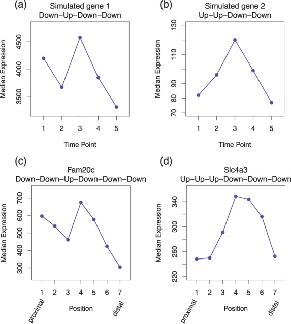
Shown are two genes identified exclusively by EBSeq-HMM in Sim I data (upper) and in case study data (lower). The x-axis shows time points (upper) and positions on mouse limb (lower), and the y-axis shows median gene expression adjusted for library sizes

Note that although EBSeq-HMM has the highest empirical FDR among these five methods, it is still well-controlled under the 5% target FDR. In fact, among all approaches, the empirical FDR from EBSeq-HMM is closest to the target FDR. To better understand the overall performance of each method, the third column in Table 1 shows the F1 score. The F1 score measures a test’s accuracy accounting for both power and false discoveries, where an F1 score reaches its best value at 1 and worst at 0. EBSeq-HMM has the highest F1 score among all approaches.

In addition, Table 1 shows that [consistent with other studies (Nueda et al., 2014)], the suggested threshold of maSigPro ($R^2=0.7$) is conservative and provides lower power than EBSeq-HMM, EBSeq, DESeq2, edgeR and voom. The power is improved by relaxing the threshold, but is still lower than others. The FC analysis works best at threshold 1.3, but is still inferior to the other methods.

Table 2 shows the power, FDR and F1 score for identifying DE genes (either dynamic or sporadic) in Sim II where, again, the target FDR is controlled at 5%. The increased power of EBSeq-HMM in identifying dynamic genes that was demonstrated in Sim I persists when sporadic genes are present, and EBSeq-HMM also shows advantage for identifying sporadic genes.

Table 2.

Operating characteristics for identifying changes in Sim II

	Power (%)	FDR (%)	F1 score (%)	Power (strong) (%)	Power (weak) (%)	Power (sporadic) (%)
EBSeqHMM	94.5	4.5	95.0	99.7	97.4	86.4
EBSeq	81.4	0.1	89.7	93.9	86.1	64.2
DESeq2	84.1	0	91.4	95.2	89.3	67.9
edgeR	84.4	0	91.6	95.4	89.5	68.3
voom	83.2	0	90.8	95.0	88.7	65.9
maSigPro (0.7)	33.1	0	49.7	56.0	37.8	5.5
maSigPro (0.5)	56.8	0.1	72.4	81.6	70.6	18.2
maSigPro (0.3)	67.4	0.5	80.4	89.9	82.3	30.0
FC (2.5)	0.4	0.4	0.8	0.7	0.4	0.1
FC (2)	2.5	1.9	4.9	4.2	2.5	0.8
FC (1.5)	36.1	4.0	52.5	55.9	28.6	23.9
FC (1.3)	83.0	9.0	86.8	97.4	82.5	69.2
FC (1.2)	95.8	20.1	87.1	99.8	97.9	89.6

The first three columns show the average power, FDR and F1 score for detecting DE genes in Sim II. For dynamic genes, the power within the strong and weak groups is further evaluated in columns 4 and 5. Power within the sporadic group is evaluated in column 6. Averages are calculated over 100 Sim II simulations. The standard errors (not shown) for EBSeq-HMM, EBSeq, DESeq2, edgeR, voom and maSigPro (and in most cases FC) were $\le 0.005$.

In spite of this advantage, we note that all methods show reduced power for identifying sporadic genes. This is because in the simulation (and in our case study data upon which the simulation is based), the range of expression differences in sporadic genes is smaller, in general, than in dynamic genes. For example, consider dynamic genes having fold changes at each transition between 1.3 and 1.4. On average, for a dynamic gene that is monotonically increasing, the range in expression would be $\sim {135}^4=332$ over all conditions (for a weak dynamic gene, the range would be $\sim 2.44$). However, in a sporadic gene, the range would be $\sim 1.35$ since only one condition differs from the others.

In addition to identification of DE genes, we also evaluated the ability of EBSeq-HMM and FC to classify genes into distinct expression paths (EBSeq, DESeq2, edgeR, voom and maSigPro were not evaluated as they were not developed for this purpose; Section 2.6). Figure 3 shows results for eight dynamic paths simulated in Sim I; these eight were chosen as they contain the most genes among all simulated paths. The ground truth shows the number of genes simulated in each expression path. Also shown are the average number classified into each path by EBSeq-HMM and by FC analysis at FC threshold K = 1.2 and 1.3 (averages are calculated over 100 Sim I datasets). Correct classifications are shown in blue; incorrect are shown in red. For FC analysis, we chose 1.2 and 1.3 as they performed best under all thresholds considered. As shown, EBSeq-HMM identified more true positives than FC, while the FDR is well below 5%. Similar results were observed in Sim II data (Supplementary Fig. S2).

Fig. 3.

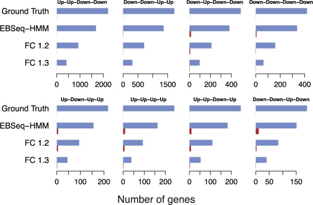
Shown are the number of genes (ground truth) simulated in Sim I as being in each of eight dynamic paths (these eight are shown as they contain the most genes among all simulated paths). Also shown are the average number classified into each path by EBSeq-HMM and by FC analysis at thresholds 1.2 and 1.3 (averages are calculated over 100 Sim I datasets). Correct classifications are shown in blue (first bar); incorrect are shown in red (second bar)

3.2 Case study results

An important problem in regenerative biology is understanding the connection between gene expression patterns and the positional identities of cells throughout development. Once humans and other mammals reach adulthood, they possess a very limited ability to regenerate body parts like limb structures; and it has been hypothesized that a loss of positional identity information is at least partially responsible for the reduction in regenerative capacity. However, a few studies (Chang, 2009; Rinn et al., 2006; Wang et al., 2009) have demonstrated that some aspects of positional identity in mammals are retained into adulthood. Understanding the changes in gene expression across limb positions in mammals is an essential first step in gaining a better understanding of these processes. Toward this end, we conducted RNA-seq experiments to study gene expression changes over seven positions (proximal to distal) along the limbs of adult mice.

EBSeq-HMM, EBSeq, DESeq2, edgeR and voom identified 14 817, 12 825, 11 517, 9520 and 10 259 DE genes at a 5% target FDR, and there is substantial overlap among the lists. Specifically, EBSeq-HMM identified over 90% of the genes identified by the other approaches. maSigPro identified 2479, 6919 and 10 727 DE genes using R² threshold 0.7, 0.5 and 0.3 and FC analyses identified 4225, 6500, 10 881, 14 016 and 15 877 genes for $K=$ 2.5, 2, 1.5, 1.3 and 1.2, respectively. These identifications showed substantially lower overlap with other methods.

Given that the majority of genes identified by EBSeq, DESeq2, edgeR and voom are also identified by EBSeq-HMM, we focus initially on genes that are identified exclusively by EBSeq-HMM. Figure 2c and d shows two examples. As in the simulated data [shown in (a) and (b)], these genes have subtle but consistent changes over the seven limb positions, again demonstrating that by accommodating dependence, EBSeq-HMM has increased power to identify genes showing relatively weak, but consistent, changes. Supplementary Figure S3 shows similar results for other genes identified exclusively by EBSeq-HMM.

Although the simulation and case study results suggest that EBSeq-HMM has increased power for identifying DE genes, the main advantage of EBSeq-HMM over other approaches is in its ability to classify genes into particular expression paths. To illustrate, we consider Hox genes, a set of genes that are of primary interest here as they are well-known to play an important role in maintaining positional identity in adult cells (Rinn et al., 2006; Wang et al., 2009). In our case study data, 33 out of 39 Hox genes were identified as DE by EBSeq-HMM. Figure 4 shows expression levels of the 33 genes along with their most likely expression paths. Although the positional changes for most Hox genes are not well-known, it is known that Hoxb4 and Hoxb8 have up-regulated expression in proximal sites (Rinn et al., 2006; Wang et al., 2009). The EBSeq-HMM paths for these genes are consistent with these prior studies and provide further information as they characterize changes across the seven positions. In addition, the overall pattern of Hox gene expression found here demonstrates that, in general, higher numbered Hox genes are up-regulated distally and lower numbered Hox genes are up-regulated proximally. This is in agreement with existing data and models of proximal-distal patterning of the limb (Zakany and Duboule, 2007).

Fig. 4.

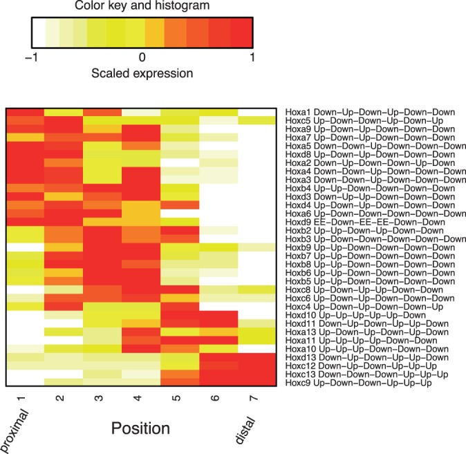
Shown are median expression levels of 33 Hox genes identified as DE by EBSeq-HMM. The expression values were adjusted for library size and further scaled to mean 0 and standard deviation 1 for each gene; median expression over three replicates is shown. Genes were clustered via hierarchical clustering using Euclidean distance and complete linkage. The x-axis shows seven positions over the mouse limb

To explore other genes beyond the Hox family that may be involved in positional identity, we considered 2347 genes that are classified by EBSeq-HMM into one of 64 possible dynamic paths. Among the 64 clusters formed by these dynamic genes, the two largest are Up-Down-Up-Down-Down-Down (827) and Down-Up-Down-Up-Up-Up (218). Figure 5a and b shows median expression of each position for each of these genes. As these groups each contain Hox genes but also previously unknown genes showing similar dynamics across position, the novel identifications define candidates for further study.

Fig. 5.

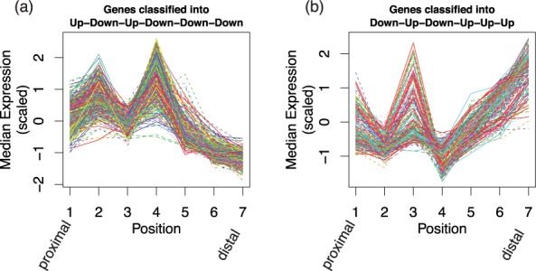
(a), (b) Shown are genes classified as following an Up-Down-Up-Down-Down-Down (left panel, 827 genes) or Down-Up-Down-Up-Up-Up (right panel, 218 genes) expression path in the case study data. Each line indicates one gene. The x-axis shows seven positions over the mouse limb; the y-axis shows median scaled expression within each position

4 Discussion

We have developed an approach called EBSeq-HMM for analysis of ordered RNA-seq experiments. EBSeq-HMM may be used to identify genes that are DE across a set of ordered conditions and to classify genes into their most likely expression paths. There are a number of methods available for identifying DE genes that may be used when data from multiple conditions is available. EBSeq-HMM has two main advantages over these approaches. First, it accommodates dependence across ordered conditions and consequently has increased power to identify genes showing subtle, yet consistent, changes. Second, for every gene, EBSeq-HMM calculates the gene-specific PP associated with each possible expression path and in doing so allows for genes to be classified into distinct expression paths with a pre-specified FDR. Put another way, EBSeq-HMM not only identifies genes that change across conditions, but can be used to specify how they change.

Simulations demonstrated the power of EBSeq-HMM over other approaches to identify DE genes. In particular, results showed that DESeq2, edgeR and voom perform well in detecting trends and/or changes are relatively strong, but that EBSeq-HMM has increased power to identify genes showing weaker changes. EBSeq-HMM also worked well for identifying genes showing sporadic changes (where there is no dependence across ordered conditions as for some genes in Sim II). Applying maSigPro-GLM with its default cutoff for calling DE genes gave significantly reduced power than other approaches. Relaxing the cutoff improved its power, but it was still inferior to the others.

In addition to DE gene identification, EBSeq-HMM performed well for classifying genes into expression paths. We defined a gene as being in a particular path if the gene was classified as DE at FDR 5% (PP of EE was less than 0.05) and the PP of being in that path exceeded 0.5. Given the two step process, observed mis-classification rates were conservatively controlled. Note that in some cases, a DE gene may not be classified to any particular path. For example, if the last time point of a four-condition experiment is known to be noisy, a gene that is initially increasing may have equal PP, say one-third, of being Up-Up-Up, Up-Up-EE, and Up-Up-Down. This gene would be called DE with 5% FDR since PP(EE-EE-EE) < 0.05, but it would not be assigned into a particular expression path if threshold 0.5 was used. In some cases, a user may want to modify these thresholds. If a false negative classification was considered more serious than a false positive, this threshold could be adjusted. Motivation for doing so under varying loss functions is discussed in (Berger, 1985).

5 Implementation

EBSeq-HMM is implemented as an R package (EBSeqHMM), currently available at Bioconductor: www.bioconductor.org/packages/devel/bioc/html/EBSeqHMM.html. EBSeq-HMM requires estimates of gene or isoform expression, but is not specific to any particular estimation method. To estimate library sizes, EBSeq-HMM defaults to median-of-ratios normalization (Anders and Huber, 2010); TMM (Robinson and Oshlack, 2010) and Upper Quartile Normalization (Bullard et al., 2010) are also available in the package.

Like most methods, EBSeq-HMM makes assumptions regarding the distribution governing expression measurements. Consequently, poor performance may result if there are strong departures from these assumptions. Model diagnostics are implemented in EBSeq-HMM to ensure that assumptions can be easily checked. They should be considered with each application and results should not be used if serious departures from model assumptions are observed. A typical diagnostic summary for the case study data is shown in Supplementary Figure S4.

References

- Ailliot P., Monbet V. (2012) Markov-switching autoregressive models for wind time series. Environ. Model. Softw., 30, 92–101. [Google Scholar]
- Anders S., Huber W. (2010) Differential expression analysis for sequence count data. Genome Biol., 11, R106. [DOI] [PMC free article] [PubMed] [Google Scholar]
- Benjamini Y., Hochberg Y. (1995) Controlling the false discovery rate: a practical and powerful approach to multiple testing. J. R. Stat. Soc.Ser. B (Methodological), 57, 289–300. [Google Scholar]
- Berger J.O. (1985) Statistical Decision Theory and Bayesian Analysis . Springer Science & Business Media. [Google Scholar]
- Bullard J.H., et al. (2010) Evaluation of statistical methods for normalization and differential expression in mRNA-seq experiments. BMC Bioinformatics, 11, 94. [DOI] [PMC free article] [PubMed] [Google Scholar]
- Chang H. (2009) Anatomic demarcation of cells: genes to patterns. Science, 326, 1206–1207. [DOI] [PubMed] [Google Scholar]
- Conesa A., et al. (2006) maSigPro: a method to identify significantly differential expression profiles in time-course microarray experiments. Bioinformatics, 22, 1096–1102. [DOI] [PubMed] [Google Scholar]
- Derrien T., et al. (2012) Fast computation and applications of genome mappability. PLoS One, 7, e30377. [DOI] [PMC free article] [PubMed] [Google Scholar]
- Ernst J., et al. (2005) Clustering short time series gene expression data. Bioinformatics, 21(Suppl. 1), i159–i168. [DOI] [PubMed] [Google Scholar]
- Filkov V., et al. (2002) Analysis techniques for microarray time-series data. J. Comput. Biol., 9, 317–330. [DOI] [PubMed] [Google Scholar]
- Glaus P., et al. (2012) Identifying differentially expressed transcripts from RNA-seq data with biological variation. Bioinformatics, 28, 1721–1728. [DOI] [PMC free article] [PubMed] [Google Scholar]
- Hamilton J.D. (1989) A new approach to the economic analysis of nonstationary time series and the business cycle. Econometrica, 357–384. [Google Scholar]
- Hardcastle T.J., Kelly K.A. (2010) baySeq: empirical Bayesian methods for identifying differential expression in sequence count data. BMC Bioinformatics, 11, 422. [DOI] [PMC free article] [PubMed] [Google Scholar]
- Koehler R., et al. (2011) The uniqueome: a mappability resource for short-tag sequencing. Bioinformatics, 27, 272–274. [DOI] [PMC free article] [PubMed] [Google Scholar]
- Langmead B., et al. (2010) Ultrafast and memory-efficient alignment of short DNA sequences to the human genome. Genome Biol., 10, R25. [DOI] [PMC free article] [PubMed] [Google Scholar]
- Law C.W., et al. (2014) Voom: precision weights unlock linear model analysis tools for RNA-seq read counts. Genome Biol., 15, R29. [DOI] [PMC free article] [PubMed] [Google Scholar]
- Leng N., et al. (2013) EBSeq: an empirical Bayes hierarchical model for inference in RNA-seq experiments. Bioinformatics, 29, 1035–1043. [DOI] [PMC free article] [PubMed] [Google Scholar]
- Li B., Dewey C.N. (2011) RSEM: accurate transcript quantification from RNA-seq data with or without a reference genome. BMC Bioinformatics, 12, 323. [DOI] [PMC free article] [PubMed] [Google Scholar]
- Love M.I., et al. (2014) Moderated estimation of fold change and dispersion for RNA-seq data with DESeq2. Genome Biol., 15, 550. [DOI] [PMC free article] [PubMed] [Google Scholar]
- Luan Y., Li H. (2003) Clustering of time-course gene expression data using a mixed-effects model with b-splines. Bioinformatics, 19, 474–482. [DOI] [PubMed] [Google Scholar]
- Ma P., et al. (2009) Identifying differentially expressed genes in time course microarray data. Stat. Biosciences, 1, 144–159. [Google Scholar]
- Nueda M.J., et al. (2014) Next maSigPro: updating maSigPro bioconductor package for RNA-seq time series. Bioinformatics., 30, 2598–2602. [DOI] [PMC free article] [PubMed] [Google Scholar]
- Rinn J., et al. (2006) Anatomic demarcation by positional variation in fibroblast gene expression programs. PLoS Genet., 2, e119. [DOI] [PMC free article] [PubMed] [Google Scholar]
- Robinson M.D., Oshlack A. (2010) A scaling normalization method for differential expression analysis of RNA-seq data. Genome Biol., 11, R25. [DOI] [PMC free article] [PubMed] [Google Scholar]
- Robinson M.D., Smyth G.K. (2007) Moderated statistical tests for assessing differences in tag abundance. Bioinformatics, 23, 2881–2887. [DOI] [PubMed] [Google Scholar]
- Robinson M.D., et al. (2010) edgeR: a bioconductor package for differential expression analysis of digital gene expression data. Bioinformatics, 26, 139–140. [DOI] [PMC free article] [PubMed] [Google Scholar]
- Schlüter R., et al. (2005) Bayes risk minimization using metric loss functions. In: INTERSPEECH, pp. 1449–1452. [Google Scholar]
- Shi Y., Jiang H. (2013) rSeqDiff: detecting differential isoform expression from RNA-seq data using hierarchical likelihood ratio test. PLoS One, 8, e79448. [DOI] [PMC free article] [PubMed] [Google Scholar]
- Teerapabolarn K. (2008) On the negative binomial approximation to the beta-negative binomial distribution. Int. J. Contemp. Math. Sci., 3, 1213–1216. [Google Scholar]
- Trapnell C., et al. (2012) Differential analysis of gene regulation at transcript resolution with RNA-seq. Nat. Biotechnol., 31, 46–53. [DOI] [PMC free article] [PubMed] [Google Scholar]
- Wang K., et al. (2009) Regeneration, repair and remembering identity: the three Rs of Hox gene expression. Trends Cell Biol., 19, 268–275. [DOI] [PMC free article] [PubMed] [Google Scholar]
- Yuan M., Kendziorski C. (2006) Hidden Markov models for microarray time course data in multiple biological conditions. J. Am. Stat. Assoc., 101, 1323–1332. [Google Scholar]
- Zakany J., Duboule D. (2007) The role of Hox genes during vertebrate limb development. Curr. Opin. Genet. Dev., 17, 359–366. [DOI] [PubMed] [Google Scholar]
Associated Data
This section collects any data citations, data availability statements, or supplementary materials included in this article.