Abstract
We propose a new framework for design under uncertainty based on stochastic computer simulations and multi-level recursive co-kriging. The proposed methodology simultaneously takes into account multi-fidelity in models, such as direct numerical simulations versus empirical formulae, as well as multi-fidelity in the probability space (e.g. sparse grids versus tensor product multi-element probabilistic collocation). We are able to construct response surfaces of complex dynamical systems by blending multiple information sources via auto-regressive stochastic modelling. A computationally efficient machine learning framework is developed based on multi-level recursive co-kriging with sparse precision matrices of Gaussian–Markov random fields. The effectiveness of the new algorithms is demonstrated in numerical examples involving a prototype problem in risk-averse design, regression of random functions, as well as uncertainty quantification in fluid mechanics involving the evolution of a Burgers equation from a random initial state, and random laminar wakes behind circular cylinders.
Keywords: surrogate modelling, response surfaces, risk-averse design, uncertainty quantification, machine learning, big data
1. Introduction
Progress in perceptibly diverse areas of science, such as numerical analysis and scientific computing, design optimization, uncertainty quantification and statistical learning, has started to carve an emerging trend in engineering design, in which decision-making becomes increasingly more data-driven rather than merely relying on empirical formulae and expert opinion. A set of versatile tools, ranging from experiments to stochastic simulations can offer invaluable input towards not only performance optimization but also risk assessment, cost effectiveness and operational aspects of a design. A smart management of these powerful resources is expected to play a vital role, especially in the case of novel, high-performance unconventional designs where simple empirical extrapolation can provide no guarantee of optimality. However, employing ensembles of high-fidelity experiments or computer simulations for performing data-driven design optimization for realistic cases may easily become a task of prohibitive cost. A viable solution to this problem is offered by considering surrogate modelling.
A surrogate model can be simply thought of as an intermediate agent that absorbs information coming from a realization of what we consider to be as the true response of a system (up to measurement error), and is able to perform inexpensive predictions as to what the true response might look like in regions where no a priori information is available. Modern statistical learning techniques have opened the path for constructing sophisticated surrogates that are able to accurately capture intrinsic features of the response of complex engineering systems [1–3]. At the heart of surrogate-based modelling, we find classical statistical methods, such as Gaussian process regression, members of which are the so-called kriging and co-kriging predictors [4,2].
Initially introduced in geostatistics by the pioneering work of Matheron [5] and Krige [6], kriging has been a flexible and reliable tool in spatial statistics and has extensively served a widespread spectrum of applications, ranging from classical data assimilation in environmental sciences to modern machine learning techniques in robotics. However, it was the seminal work of Sacks et al. [7] that introduced kriging in the context of design and analysis of computer experiments, and consequently led to a rapidly growing field of application in which kriging has been used as a predictive tool for constructing response surfaces of engineering systems by exploring the spatial correlation between the output of deterministic computer codes. Simpson et al. [8] provide a comprehensive summary of the evolution and recent advancements of this metamodelling approach in the context of multidisciplinary design optimization.
Of particular importance to our study is the work of Kennedy & O'Hagan [9] that introduced the use of first-order auto-regressive stochastic models for predicting the output of a complex computer code when fast approximations are available. We recognize that this approach establishes a coherent mathematical framework for blending heterogeneous variable-fidelity information sources, creating a natural setting for multi-fidelity modelling. Forrester et al. [10] adopted this methodology to build a two-level co-kriging scheme and successfully applied it for optimizing the drag/dynamic pressure ratio of a transonic aircraft wing.
Although the auto-regressive scheme of Kennedy & O'Hagan [9] has served well many disciplines and applications, it suffers from the same limitations as any kriging/co-kriging method. The biggest practical limitation stems from the need to repeatedly invert large, dense, ill-conditioned covariance matrices at the machine learning stage, where the metamodel is trained on a set of known observations. To address this issue, we have aligned our work with some new interesting findings that can significantly enhance the computational efficiency of kriging/co-kriging. First, the treatise of Le Gratiet & Garnier [11] suggests that co-kriging schemes arising from the Kennedy & O'Hagan model [9] with s-levels of variable-fidelity information sources can be effectively decoupled, and equivalently formulated in a recursive fashion as s-independent kriging problems. This allows for the construction of predictive co-kriging schemes by solving a sequence of simpler kriging problems that involve covariance matrices of smaller dimensions (and potentially lower condition numbers), which can be learned from the data by performing optimization in lower dimensional spaces (compared with the coupled setting of Kennedy & O'Hagan [9]). Nevertheless, the machine learning problem for fitting a kriging metamodel to the data at each recursive step still requires the factorization of a dense covariance matrix. To this end, we note that the popular choice of Cholesky decomposition scales with the number of n observed data points as , thus rendering the learning process infeasible for large n. An efficient alternative approach for constructing and learning covariance kernels for spatial statistics was recently put forth by Lindgren et al. [12]. Their idea uses Hilbert space approximation theory to construct sparse representations of the inverse covariance of a Gaussian–Markov random field (GMRF) that solves a certain stochastic partial differential equation (SPDE). As a consequence, the kriging/co-kriging formulation can be recast in a form that exploits the sparsity in the inverse covariance, leading to significant computational savings at the model learning stage, which now scales as fast as [12].
The aim of this work is to establish a new mathematical framework for surrogate-based building of response surfaces that simultaneously takes into account multi-fidelity in models (e.g. high-fidelity direct numerical simulations versus low-fidelity empirical formulae) as well as multi-fidelity in probability space (e.g. high-fidelity tensor product multi-element probabilistic collocation versus low-fidelity sparse grid quadratures). We incorporate elements of statistical learning in an auto-regressive co-kriging methodology to cross-correlate ensembles of multi-fidelity surrogates from which we can accurately and efficiently extract the response of complex nonlinear stochastic dynamical systems. This framework targets a seamless integration of surrogate-based optimization and uncertainty quantification, providing a launch pad for contemporary engineering design under uncertainty.
This paper is structured as follows. In §2, we outline the basic mathematical concepts upon which the proposed framework is built. In particular, §2a describes the setting of multi-fidelity modelling and introduces the core concept of Gaussian process regression in the form of kriging, co-kriging and multi-level recursive co-kriging. We then define a general auto-regressive setting under which multi-fidelity in models and multi-fidelity in probability space can be addressed in unison. Subsequently, §2c presents an overview of the use of GMRFs through the SPDE approach to construct sparse approximations to the inverse covariance in order to boost the efficiency of machine learning algorithms at the model fitting stage. The capabilities of the proposed methodology are demonstrated through four benchmark problems. First, we consider a prototype problem in risk-averse design, in which we seek the optimal dimensions of a structural column with uncertain material properties that undergoes random bending and axial excitation. Second, we present results on the regression of a random function using an ensemble of multi-fidelity surrogates. Third, we study a prototype problem in multi-fidelity uncertainty quantification involving the evolution of viscous Burgers dynamics from a random initial state. Finally, we conclude with presenting an uncertainty quantification problem in fluid dynamics that involves stochastic incompressible flow past a circular cylinder.
2. Methods
We provide a brief overview of the methods we employ for constructing response surfaces by blending information sources of variable fidelity. The core concepts of our methodology lie within the broad topics of Gaussian process regression and machine learning. To this end, we begin our presentation with the univariate regression case, illustrating how spatially correlated variables can be estimated using ordinary kriging. The idea is then extended to the multivariate case, introducing the formulation of ordinary co-kriging. In particular, we focus our attention on the auto-regressive model first put forth by Kennedy & O'Hagan [9] in the context of predicting the output of a complex expensive high-fidelity code by using fast lower fidelity approximations. We show how this model can be generalized to construct a unified framework that can simultaneously address multi-fidelity in models as well as multi-fidelity in probability space. Finally, we conclude our presentation by introducing two concepts that enhance the feasibility and efficiency of computations. The first part relies on the recent contributions of Le Gratiet & Garnier [11], who proved that the s-level auto-regressive model of Kennedy & O'Hagan [9] can be equivalently formulated as s-independent kriging problems. This could potentially lead to substantial computational savings for cases where one may encounter many information sources of variable fidelity. The second part is based on the findings of Lindgren et al. [12], who employed Galerkin projection techniques to construct covariance models of GMRFs. This enables fast computations that leverage on the sparsity of the resulting discrete operators, thus suggesting an efficient algorithmic framework for handling big data at the model inference stage.
(a). Multi-fidelity modelling
Consider a general system whose response can be evaluated using different models. The response typically depends on a set of design parameters and is subject to uncertainties encoded by a set of random parameters, . Given a set of design criteria, our goal is to construct the corresponding response surface that quantifies the dependence of a derived quantity of interest, f(Y(x;ξ)), on the input design variables x and uncertainties ξ (figure 1). Design criteria come in different flavours and generally reflect our priorities and objectives in identifying configurations of the design variables x that qualify as optimal. For example, one may pursue to maximize the performance of a system for a wide range of operating conditions [13], identify a design with a probability density function (PDF) that matches a target performance [14], or minimize the risk associated with undesirable realizations [15] (table 1). All concepts introduced in the subsequent sections aim to address single-objective design optimization problems, where the quantity of interest is the output of a scalar function of the inputs. This can serve as a basis for extending the proposed methodology to multi-objective problems, where the quantity of interest could be a multi-dimensional vector, or even a continuous field.
Figure 1.

Schematic of the multi-fidelity design under uncertainty framework: the quantity of interest Y(x;ξ) is a random field in the design space, realizations of which could originate from information sources of variable fidelity (such as computer codes, experiments, expert opinion, etc.). A response surface S(x) encodes the dependence of a derived quantity of interest f(Y(x;ξ)) on the input design variables x and uncertain parameters ξ. The ability to efficiently construct response surfaces (e.g. ) allows one to asses the system's performance as a function of the random inputs and identify optimal configurations based on the desired design criteria (table 1). (Online version in colour.)
Table 1.
Examples of possible design criteria.
The process usually referred to as multi-fidelity modelling, elaborates on efficiently constructing response surfaces by correlating surrogate models of different fidelity. On one side of the fidelity spectrum, one may have cheaper surrogate models, which are fast to compute but less trustworthy (e.g. potential flow solvers, empirical formulae, etc.), while on the other side we have high-fidelity models that enjoy our outmost trust but can be very expensive to compute (e.g. direct numerical simulations, experiments, etc.). In many cases, exploring the correlation between the two allows us to efficiently construct an accurate representation of the response surface by performing relatively few evaluations of an expensive high-fidelity model and more evaluations of a cheaper surrogate. A linking mechanism that undertakes the task of information fusion naturally arises in the context of multivariate Gaussian regression. Next, we introduce this concept in the context of ordinary kriging and co-kriging.
(i). Kriging
Here we present a brief overview of the kriging predictive scheme. The reader is referred to [1,2,4,7] for a detailed exposition of the subject. The main idea here is to model scattered observations of a field Y (x) as a realization of a Gaussian random field Z(x). These observations could be corrupted by model error or measurement noise that is described by a Gaussian process , leading to an observation model of the form
| 2.1 |
Consequently, the random field (Z(x),Y (x))T has a multivariate normal distribution
| 2.2 |
where, μ=E[Z] is the mean value of Z, Σ is the covariance of Z, is the covariance of the noise , and A is a simple matrix that restricts the random field Z(x) to the locations of observed data y. Additional assumptions on μ(x) may distinguish a linear spatial prediction model into simple Kriging (if μ is assumed to be known), ordinary Kriging (if μ is unknown but independent of x), and universal Kriging (if μ is unknown and is represented as a linear combination of deterministic basis functions) [4].
Starting from the conditional distribution of Z|Y , we can derive equations for the expectation μZ|Y(x), and covariance ΣZ|Y(x) of the ordinary kriging predictor as
| 2.3 |
and
| 2.4 |
Typically, the covariances Σ and are parametrized by a set of hyperparameters, , that can be learned from the data y by maximizing the posterior using maximum-likelihood estimation (MLE) or in a fully Bayesian setting (e.g. Markov Chain (MC) integration). This essentially introduces a machine learning problem for computing the optimal values of the unknown parameters from the data.
The noise process accounts for epistemic uncertainties that lead to differences between our observables and the real response of the system because of inaccurate or uncertain modelling assumptions. In the experimental setting this may correspond to noise or bias in the measurements, whereas in the numerical setting it may account for round-off or truncation errors of the numerical scheme. In general, modelling the nature of results in an intrinsically hard problem that is beyond the scope of this study. Without loss of generality, in what follows we will assume that is a zero-mean Gaussian white noise process with variance , i.e . This should not be confused with aleatoric uncertainties that arise from randomness in the input parameters of the system that will be taken into account by the random vector ξ (figure 1 and §2b).
(ii). Co-kriging
The idea of kriging is naturally extended to the multivariate setting, in which the observation model for Y (x) depends on more than one covariates. Here, we present a brief overview of the approach of Kennedy & O'Hagan [9], which introduced a co-kriging model based on a first-order auto-regressive relation between model output of different levels of fidelity.
Suppose we have s-levels of variable-fidelity model output at locations sorted by increasing fidelity and modelled as observations of a Gaussian field . Then, ys(x) denotes the output of the most accurate and expensive model, while y1(x) is the output of the cheapest least accurate surrogate at our disposal. The auto-regressive co-kriging scheme of Kennedy & O'Hagan [9] reads as
| 2.5 |
where δt(x) is a Gaussian field independent of {Zt−1(x),…,Z1(x)}, and distributed with expectation μδt and covariance Σt, i.e. . Also, ρ(x) is a scaling factor that quantifies the correlation between the model outputs (yt(x),yt−1(x)). In a Bayesian setting, ρ(x) is treated as a random field with an assigned prior distribution that is later fitted to the data through inference. Here, to simplify the presentation we have assume that ρ is a deterministic scalar, independent of x, and learned from the data through maximum-likelihood estimation (see §2d).
The derivation of this model is based on the Markov property
| 2.6 |
which, according to Kennedy & O'Hagan [9], translates into assuming that given Zt−1(x), we can learn nothing more about Zt(x) from any other model output Zt−1(x'), for x≠x'.
The resulting posterior distribution at the tth co-kriging level has a mean and covariance given by
| 2.7 |
where μt is the mean value of Zt(x), Σt is a covariance matrix comprising t blocks, representing all cross-correlations between levels {t,t−1,…,1} and is the covariance of the co-kriging predictor at level t. Also, σt is the variance of the noise at level t, and At is a simple matrix that restricts a realization of the Gaussian field Zt(x) to the locations of observed data yt(x) at level t. Similar to ordinary kriging, the set of unknown parameters {μt,ρt−1,…,ρ1,θt,…,θ1,σt,…,σ1} are determined from the data using machine learning techniques. To simplify the presentation, we have assumed that the scaling factor ρ attains scalar values, hence it does not depend on x. In general, we introduce a spatial dependence by using a representation in terms of a basis ϕ(x), i.e. , where the M unknown modal amplitudes w can be determined through optimization. For cases that exhibit a smooth distribution of the cross-correlation scaling, only a few number of modal components should suffice for capturing the spatial variability in ρ(x), thus keeping the computational cost of optimization to tractable levels.
Although this co-kriging framework provides an elegant way of blending variable-fidelity model output, it may easily become computationally infeasible if many levels of fidelity and/or a large number of data observations are available. The computational barrier is imposed by the need to repeatedly invert the full covariance matrix Σt at the model fitting stage, with the number of different fidelity levels resulting to an increasing matrix size, while large observation datasets introduce ill-conditioning. These are well-known limiting factors for kriging but they become even more evident for co-kriging models where the total number of observations is the sum of the observations at all fidelity levels. However, recent findings of Le Gratiet & Garnier [11] provide an equivalent formulation that overcomes the computational complexity issues of the Kennedy and O'Hagan model by decoupling the aforementioned s-level co-kriging scheme into s-independent kriging problems. The resulting recursive scheme is proved to provide a predictive mean and variance that is identical to the coupled Kennedy and O'Hagan model, although it could potentially lead to a drastic reduction of the size and condition number of the covariance matrices that need to be inverted.
The key idea behind the derivation of Le Gratiet & Garnier [11] is to replace the Gaussian process Zt−1(x) in equation (2.5) with a process that is conditioned by all the known observations {yt−1,yt−2,…,y1} up to level (t−1), while assuming that the corresponding experimental design sets have a nested structure, i.e D1⊆D2⊆⋯⊆Dt−1. Then, the problem at the tth-level reduces to an ordinary kriging predictor with mean and covariance given by
| 2.8 |
Here, we note that the hypothesis of nested design sets can be relaxed only at the expense of a more tedious derivation, and the corresponding expressions of the recursive co-kriging predictor and variance can be found in [16].
To underline the potential benefits of this approach, we note that the matrix Σt in the Kennedy and O'Hagan model (see equation (2.7)) has size , where nt is the number of observations at the tth fidelity level. On the other hand, the recursive co-kriging approach involves the inversion of s covariance matrices (see equation (2.8)) of size nt×nt, where nt is the number of observations yt(x) at level t [11]. Moreover, we note that at each recursive level, the number of unknown parameters to be learned from the data reduce to {μt,ρt−1,θt,σt} compared with the large parametric set of {μt,ρt−1,…,ρ1,θt,…,θ1,σt,…,σ1} of the coupled Kennedy and O'Hagan scheme.
(b). Multi-fidelity in models and in probability space
We can build further upon the presented co-kriging framework to formulate a general methodology that can simultaneously address multi-fidelity in physical models as well as multi-fidelity in probability space. As it is often the case in realistic design scenarios, the output of a system may well be sensitive to a set of inputs ξ that exhibit random variability. Consequently, decision-making towards identifying an optimal design is typically informed by exploring the measures of uncertainty that describe the response of the underlying stochastic dynamical system. This response is often characterized by non-Gaussian statistics that can be estimated numerically by using appropriate sampling and integration techniques. The potential non-Gaussianity in the system response should not be confused with the Gaussian nature of the kriging/co-kriging predictors. The former is an inherent property of the dynamical system that generates the observed data, while the latter introduces a modelling framework for information fusion.
Similar to having multi-fidelity in models, methods of different fidelity can also be incorporated in probability space to provide an accurate quantification of uncertainty introduced by random input. This structure is schematically illustrated in figure 2, where m models of variable fidelity in physical space are driven by random input, hence producing a random response surface Ym(x;ξ). In return, any uncertainty quantification measure of Ym(x;ξ), such as for e.g. the expectation or the risk , can be estimated using a set of p variable-fidelity methods (figure 2). In our framework, the challenge of high stochastic dimensionality is reflected by the accuracy and efficiency of the approximation methods employed to quantify uncertainty in the system. Essentially, this is a high-dimensional integration problem arising in the computation of quantities such as expectation, variance, risk measures, etc. To this end, the practical scalability of our approach can directly benefit from established techniques for high-dimensional integration, such as MC integration [17] or ANOVA decomposition methods [18] (figure 3).
Figure 2.

Multi-fidelity in models and in probability space: m models of variable fidelity in physical space are driven by random input, producing a random response surface Ym(x;ξ). For example, the expectation of a derived quantify of interest can be estimated by employing p methods of variable fidelity in probability space. (Online version in colour.)
Figure 3.
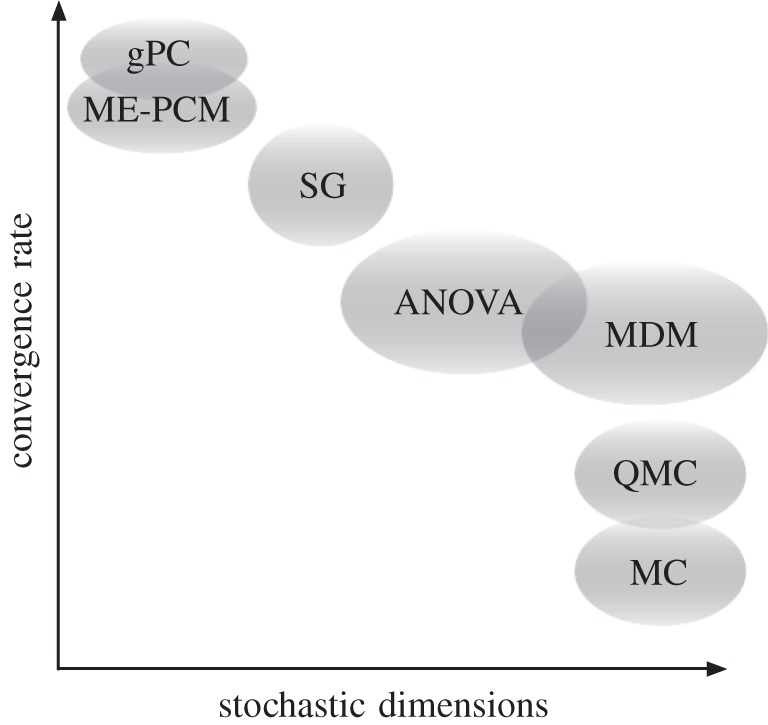
Multi-fidelity in probability space: a non-exhaustive collection of methods in probability space sorted as a function of their convergence rate and practical scalability to high dimensions: generalized polynomial chaos (gPC [19]), multi-element probabilistic collocation (ME-PCM [20]), sparse grids (SG [21]), ANOVA decomposition methods [18], multivariate decomposition methods (MDM [22]), quasi-Monte Carlo (QMC [17]) integration and Monte Carlo (MC [17]) integration.
This construction results in a family of response surfaces that can be organized hierarchically in a p×m matrix, where physical model fidelity is increased along the columns and probability space model fidelity increases along the rows (figure 4). Then, it is meaningful to allow information fusion along the directions by employing the auto-regressive co-kriging framework presented in §2a(ii). For example, moving along the purely vertical direction {↓} results to the following auto-regressive expression for the expectation :
| 2.9 |
where the k-index increases with the fidelity of the estimator of in probability space, while the l-index increases with model fidelity in physical space. Note that the recursive co-kriging scheme allows for sequentially decoupling the inference process to a number of independent steps. The last of these steps should always involve the quantity of interest , as our goal is to construct an accurate representation of the highest fidelity model. However, the intermediate steps need not involve , as their purpose is to sequentially improve the predictor at a level (k<p,l<m) by conditioning on observations of a lower level. Essentially, equation (2.9) provides an example of an intermediate step in which the predictor of level (k+1,l) is enhanced with any correlated information contained in level (k,l).
Figure 4.

Family of response surfaces resulting from simultaneously addressing multi-fidelity in models and in probability space. Physical model fidelity is increased along the columns (red arrow) and probability space model fidelity increases along the rows (blue arrow). The yellow arrow represents a possible optimal information fusion path in the combined fidelity space. (Online version in colour.)
This structure gives rise to the very interesting task of identifying an optimal path traversal between different models for building an accurate representation of the target response surface. This is an open question that we plan to address in a future study. A possible way of attacking this problem is through stochastic dynamic programming techniques for guiding an optimal allocation of available computational resources [23]. Alternatively, one could employ random graph theory to identify optimal information/entropy diffusion paths, where each graph node is weighted by the fidelity and corresponding cost of each model, while edge weights represent the degree of correlation between different models.
Here, we underline that the auto-regressive structure essentially explores spatial cross-correlations between two different fidelity levels, with the target goal being the construction of an accurate estimate for the highest fidelity level. This implies that the user should be able to provide a consistent labelling of different fidelity levels, suggesting that information fusion is considered to be meaningful only when moving from a lower to higher fidelity. If the lower fidelity levels cannot provide information that is spatially correlated to the highest fidelity observations, the co-kriging predictor is likely to return an estimate comparable with a standard kriging scheme through the highest fidelity points. However, the proposed auto-regressive framework provides a mechanism for detecting this pathology, and that is done by monitoring the scaling factor ρ appearing in the auto-regressive scheme (which is learned from the data). Values of ρ away from 1 provide an indication of weak correlation between two levels, thus suggesting revision of the available models.
(c). Gaussian–Markov random fields and the stochastic partial differential equation approach
Kriging and co-kriging methods provide predictive schemes that are constructed by exploring spatial correlations between variables. A key part of this process is fitting a parametric covariance model to the observed data using machine learning and optimization techniques. The main cost of this procedure is the factorization of dense and often ill-conditioned covariance matrices for estimating the likelihood functions that guide the machine learning algorithm. Here, we provide a brief overview of a method that can effectively reduce the cost of inferring covariance models from input data, leading to efficient kriging and co-kriging predictive schemes.
A popular choice of a kernel characterizing the covariance of a random field u(x) stems from the Matérn family [4,2],
| 2.10 |
where ν determines the mean-square differentiability of u(x), κ is a scaling parameter related to the correlation length of u(x), denoted by ρ, and defined as . Also, σ2 is the marginal variance of the process, while Γ(⋅) and Kν(⋅) are the Euler gamma and modified Bessel function of the second kind, respectively. We note that for ν=0.5, the Matérn covariance simply reduces to the exponential covariance kernel, while when we recover the Gaussian kernel [4,2].
A powerful result by Whittle [24] shows that a random field u(x) with a Matérn covariance is a solution to the fractional SPDE
| 2.11 |
where is Gaussian white noise, and τ is a scaling parameter. Admissible solutions to equation (2.11) are referred to as Matérn fields and are proved to be the only stationary solutions to this SPDE [24].
A key idea put forth by Lindgren & Rue in [12] is to employ Hilbert space approximation theory to approximate the solution to equation (2.11) using a projection onto a finite dimensional space spanned by basis functions ϕ1(x),…,ϕN(x) as
| 2.12 |
where {wk} are a set of unknown Galerkin expansion coefficients.
A critical observation of Lindgren & Rue in [12], citing the work of Rozanov [25], states that a random field has a Markov property if and only if the reciprocal of its spectrum is a polynomial. Thereby, the Matérn fields generated by equation (2.11), inherit the Markov property when α assumes integer values. Exploiting this Markov property, Lindgren & Rue [12] were able to use the finite dimensional approximation of u(x) given in equation (2.12) to construct a GMRF with precision matrix Q that approximates the Gaussian field u(x) in the sense that Q−1 is close to the covariance of u(x), denoted by Σ [12]. The main advantage here is that the Markov property, along with the choice of a suitable basis, results in a sparse precision matrix Q (figure 5), and, thus, enables the use of fast numerical methods for sparse matrices. This allows us to recast the kriging/recursive co-kriging formulae (equation (2.3), (2.8)) in terms of sparse GMRF precision matrices obtained from a finite-element discretization of the SPDE (equation (2.11)) in the design space. To this end, the fully discrete form of the SPDE reads as
| 2.13 |
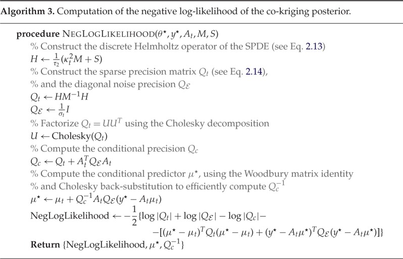
where H=κ2M+S is the discrete Helmholtz operator, M and S are the mass and stiffness matrices, w is a vector containing the unknown Galerkin coefficients of the expansion in equation (2.12), while g is the projection of the right-hand side Gaussian white noise forcing term. Then, according to Lindgren & Rue [12], the sparse GMRF precision matrix of the finite-element solution to equation (2.11) can be obtained recursively for integer values of α as
| 2.14 |
| 2.15 |
| 2.16 |
Figure 5.
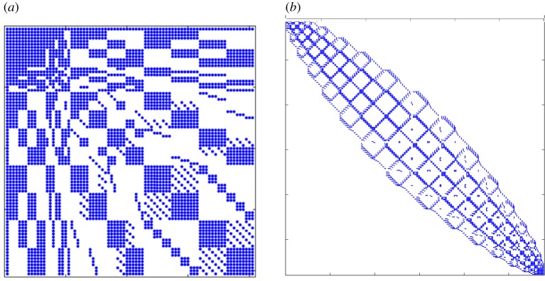
Sparsity patterns of GMRF precision matrices (α=2): (a) Q2 in a two-dimensional square domain discretized by eight quadrilateral elements using a fifth-order polynomial expansion basis. (b) Q2 in a two-dimensional square domain discretized by four quadrilateral elements using a second-order polynomial expansion basis with the corresponding degrees of freedom being re-ordered using the Cuthill–McKee bandwidth reduction algorithm [26]. (Online version in colour.)
In what follows, we assume that α=2. As the design space for all cases considered in this study is two-dimensional, this corresponds to assuming that the predicted response surfaces have continuous derivatives up to second order in the mean-square sense. Here, we also note that deriving proper stochastic boundary conditions for closing the SPDE of equation (2.11) is an active area of research. In practice, equation (2.11) is typically solved using zero Neumann boundary conditions, although this results in numerical boundary layer errors on the covariance of the solution that decay to zero at a distance equal to the correlation length of the random field u(x) away from the boundary [12]. This drawback can be alleviated by smoothly extruding the domain boundaries away of the region of interest, and avoiding spatial discretizations with sharp corners.
The main advantage of using GMRFs through the SPDE approach is that the model inference and kriging prediction stages can be completed simultaneously with cost for arbitrary geometries in two dimensions, and with cost for two-dimensional spatio-temporal kriging problems and arbitrary geometries in three dimensions [12], where m is the sum of both the number of observed data points as well as the points where kriging/co-kriging predictions are sought. This can be achieved by employing a Cholesky or pivoted Cholesky decomposition for sparse matrices, the efficiency of which depends on the bandwidth of the precision matrix. In order to further exploit this property, we can re-order the degrees of freedom in Q using a bandwidth reduction procedure, such as the Cuthill–McKee algorithm [26] (figure 5b).
Despite the fact that GMRF-based inference schemes are not a necessary ingredient of the proposed mixed multi-fidelity methodology, they can provide an effective way of handling big data in two and three dimensions, thus circumventing one of the main limitations of the kriging/co-kriging methods, i.e the general cost of factorizing dense, ill-conditioned covariance matrices. In higher dimensions, one may still adopt this approach by using, for example, a global expansion based on tensor products of an orthogonal basis. Of course, such analysis introduces some limitations, as it is restricted to hypercube domains, and the observed data need to be located (or interpolated) at the collocation points introduced by the global expansion. An alternative approach to addressing high-dimensionality is to employ a data-driven dimensionality reduction technique. To this end, one may construct latent variable models through principal component analysis (PCA), nonlinear PCA, projection-pursuit methods and ANOVA decomposition methods [3] towards identifying a new optimal set of input coordinates that spans a space of lower dimension. Finally, it is worth mentioning that the SPDE approach can be straightforwardly extended to construct more general GMRF models that are capable of addressing complex response features, such as anisotropy and non-stationarity [12].
(d). Sampling strategies and workflow
In this work, we have employed standard infill strategies, mainly relying on uniform random sampling or Latin Hypercube sampling (LHS). In the context of performing inference using GMRFs through the SPDE approach, we construct a tessellation of the input space using triangular/quadrilateral finite-elements in two dimensions, or prismatic/hexahedral/tetrahedral elements in three dimensions, where both sampling and test locations define vertices in the mesh and are chosen with the goal of maintaining a non-degenerate geometric aspect ratio within each element.
In general, a space filling strategy such as LHS can typically serve as a good starting point, followed by a subsequent refinement that is guided by the objectives and problem at hand. For example, if the goal is to locate the global minimum of the response surface one may employ a sampling strategy based on maximizing the expected improvement of the recursive co-kriging predictor [27]. A discussion on possible ways of determining a good allocation of points among different levels has been provided in the treatise of Le Gratiet & Garnier [16], although we believe this is still an open question that is tightly related to the given problem and objectives.
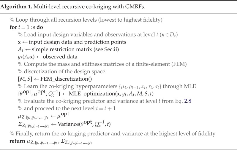
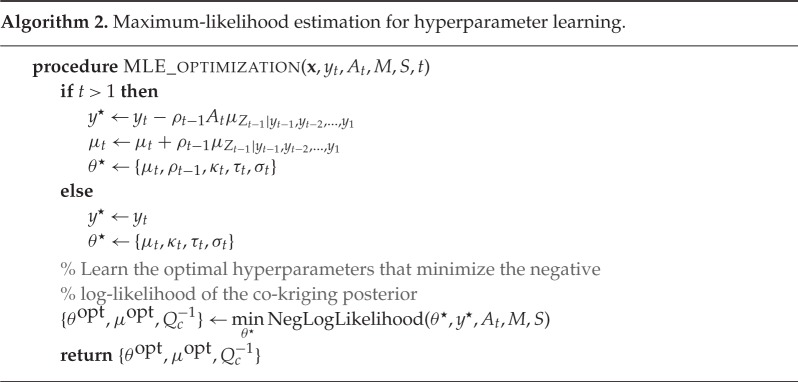
In view of available multi-fidelity data, algorithms 1–4 summarize the main implementation aspects of the proposed multi-level co-kriging framework, formulated using sparse GMRF precision matrices. Namely, we provide pseudocode for the main co-kriging recursion loop (see algorithm 1), the hyperparameter learning through maximum-likelihood estimation (see algorithm 2), the computation of the negative log-likelihood function of the co-kriging posterior (see algorithm 3), and the computation of the co-kriging variance (see algorithm 4).

3. Results
(a). A prototype problem in risk-averse design
Consider a rectangular cross section of a short structural column, with depth x1 and width x2, under uncertain yield stress and uncertain bending and axial loads. Assuming an elastic-perfectly plastic material, a limit state function that quantifies a relationship between loads and capacity is described by the random field [28]
| 3.1 |
where the bending moment load ξ1, the axial load ξ2 and the material yield stress ξ3 are distributed as
Note that lower values of Y indicate more favourable capacity-to-load ratios, while high values correspond to critical regimes where failure may occur. Our aim here is to identify an optimal configuration in the two-dimensional design space D1×D2=[2,20]×[2,10] that satisfies a set of prescribed criteria. Here, we let this goal translate to identifying a design that minimizes the area of the column with the associated design risk staying below a given threshold c. To quantify the risk associated with a given response Y (x;ξ), we employ a superquantile risk measure, which for a parameter α∈[0,1) is defined as [15]
| 3.2 |
For α=0, the superquantile risk measure of a continuously distributed random field Y (x;ξ), reduces to the expectation operator, i.e. , thus characterizing a risk-neutral situation. However, for non-zero values α∈(0,1), the superquantile risk of Y (x;ξ) returns the average of the (1−α)% highest realizations of Y (x;ξ), therefore informing a risk-averse decision-making mindset [15].
The design problem can be formulated in a constrained minimization framework which reads as
| 3.3 |
The expectation operator appearing in the computation of the superquantile risk can be approximated using a variety of different probabilistic methods of different cost and fidelity. Here, we choose to discretize the three-dimensional parametric space of (ξ1,ξ2,ξ3) using two different models. The high-fidelity model is a probabilistic collocation method (PCM) [20] on a tensor product grid with 10 quadrature points along each random dimension (total of 103 quadrature points), while the low-fidelity model is a Smolyak sparse grid level-2 quadrature (SG-L2) [21] with a total of only 58 quadrature points.
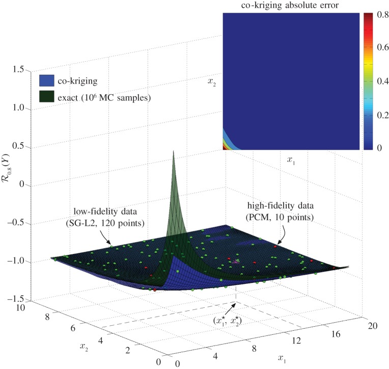
This set-up yields a simple application of the proposed multi-fidelity methodology, where we have a single model in physical space (equation (3.1)) and two levels of fidelity in probability space (PCM, SG-L2). Employing a two-level recursive co-kriging algorithm (see §2a(ii)), we can explore the correlations between the two probabilistic models, and build an accurate representation of the target response surface by mainly using the realizations of the lower fidelity model (SG-L2, 120 points in design space), guided by few realizations of the higher fidelity model (PCM, 10 points in design space).
In figure 6, we present the computed response surface as a function of the design variables (x1,x2) considering the 20% highest realizations of Y . The exact solution corresponds to computing using 106 MC samples [17]. The resulting response surface becomes singular as , while it attains a very flat profile in the rest of the design space. This flat behaviour suggests that the identification of an optimal design as a solution to equation (3.3) is highly sensitive to the accuracy of the computed response surface. Here, we have chosen a design criterion of , yielding an optimal solution for that does not depend on further resolution refinement.
Figure 6.
Exact response surface and co-kriging predictor constructed using 120 low-fidelity (SG-L2) and 10 high-fidelity (PCM) observations. denotes the optimal solution to the optimization problem of equation (3.3), while the inset plot shows the point-wise absolute error of the co-kriging predictor. (Online version in colour.)
Although this is a pedagogical prototype case in risk-averse design under uncertainty, it does not fully reflect the strengths of the proposed multi-fidelity framework as the two probabilistic methods (PCM, SG-L2) both happen to produce very similar estimations of the mean . The next example illustrates better the capabilities of the proposed methodology in the context of multi-fidelity regression of a random function.
(b). Multi-fidelity regression of a random function
Here, we consider a system with two input design variables x=(x1,x2), subject to external uncertainties, described by four standard normal random variables ξ=(ξ1,ξ2,ξ3,ξ4). Let the response of this system, denoted by Y (x;ξ) be described by the random function
| 3.4 |
Now, assume that fe(x;ξ) returns the real high-fidelity response but is expensive to evaluate. On the other hand, let fc(x;ξ) be a low-fidelity cheap to evaluate surrogate model that we can sample extensively as
| 3.5 |
Our goal here is to employ the proposed multi-fidelity framework to construct the response surface of the mean field . In order to approximate the expectation operator, we employ two methods of different fidelity in probability space. To this end, we choose our high-fidelity probabilistic method to be a Smolyak sparse grid level-5 quadrature (SG-L5) [21] that discretizes the four-dimensional parameter space using 4994 quadrature points. Similarly, the low-fidelity method in probability space is a coarser, lSG-L2 with just 57 quadrature points [21].
Therefore, our multi-fidelity setup consists of two models in physical space (fe(x;ξ),fc(x;ξ)), and two models in probability space (SG-L5, SG-L2). This results in a family of response surfaces Sij, that can be organized as
| 3.6 |
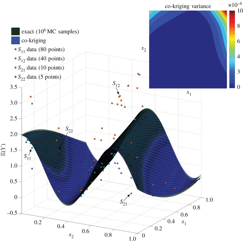
Figure 7 demonstrates the response surface produced using a four-level recursive co-kriging scheme, traversing the available models and data in the order , i.e. from lowest to highest fidelity. The resulting response surface is compared with an ‘exact’ solution that is obtained by MC integration of the high-fidelity physical model fe(x;ξ) using 106 samples. Evidently, the highly nonlinear response of the mean field is captured remarkably well by just using five observations of the expensive highest fidelity model S22, supplemented by a number of inaccurate low-fidelity observations from (S11,S12,S21). This observation is further confirmed by the uncertainty of the predictor, quantified by the co-kriging variance (figure 7, inset), which is bounded by 10−3. To underline the merits of using the proposed multi-fidelity approach note that the relative error between the exact solution and the four-level co-kriging predictor is 10−2. This is in sharp contrast with the corresponding error from fitting a kriging model through the highest fidelity observations S22, which here is as high as 0.5.
Figure 7.
Exact response surface and co-kriging predictor constructed using four levels of fidelity: 80 S11 points (fc(x;ξ), SG-L2), 40 S12 points (fc(x;ξ), SG-L5), 10 S21 points (fe(x;ξ), SG-L2) and five S22 points (fe(x;ξ), SG-L5). The inset plot shows the point-wise variance of the co-kriging predictor. (Online version in colour.)
(c). Multi-fidelity uncertainty quantification in a stochastic Burgers equation
Let us consider the following prototype initial/boundary value problem for the Burgers equation in one input dimension
| 3.7 |
where is a viscosity parameter, while the random initial condition u0(x;ω) and the deterministic forcing term f(x,t) are defined as
| 3.8 |
and
| 3.9 |
For each realization of u0(x;ω), the solution u(x,t;ω) takes values in the space , on which equation (3.7) is endowed with periodic boundary conditions. Moreover, the initial state is characterized by a unit mean and variance, i.e. , , ∀x.
Our goal here is to use the proposed multi-fidelity framework to get an accurate estimate of the kinetic energy
| 3.10 |
To this end, we consider blending the output of an ensemble of variable-fidelity models in physical and probability space. In physical space, we employ Fourier–Galerkin discretizations of equation (3.7), where higher fidelity models are obtained by increasing the number of modes N in the finite-dimensional representation of the solution:
| 3.11 |
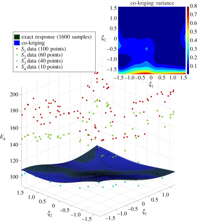
The uncertainty introduced by the two uniform random variables (ξ1,ξ2) in equation (3.8) is resolved by different probabilistic approximation methods. Here, we have employed a high-fidelity tensor product PCM, and several low-fidelity approximations based on MC integration using relatively small numbers of samples. In particular, we have considered four levels of mixed fidelity in physical and probability space. For the first level, labelled as S1, we have considered a low resolution discretization in physical space using only 10 Fourier modes in equation (3.11). This yields an inaccurate solution of equation (3.7), but results in a very low computational cost per sample, thus motivating the use of a high-fidelity method in probability space that discretizes the parametric space with 1600 PCM quadrature points. At the second level, S2, we employ a slightly finer resolution in physical space using 12 Fourier modes, while we decrease the fidelity in probability space by employing MC integration on 60 samples. Similarly, the discretization of the third level, S3, output consists of 15 Fourier modes in physical space, and 40 MC samples. Lastly, in the fourth level, S4, we employ a costly high-fidelity representation in physical space using 60 Fourier modes, but all probabilistic quantities are inferred by using only 10 MC samples.
Figure 8 presents the resulting four-level recursive co-kriging predictor and variance for the multi-fidelity reconstruction of the kinetic energy Ek(t;ω) at t=1 as a function of the random variables ω=(ξ1,ξ2). The inference scheme at each recursive level is formulated using sparse GMRF precision matrices arising from a regular finite element discretization of the (ξ1,ξ2) plane with 1600 elements. It is evident that the proposed methodology is able to return an accurate estimate primarily based on a large number of inexpensive but inaccurate evaluations, supplemented by just a few realizations of the accurate but expensive high-fidelity model.
Figure 8.
Stochastic Burgers equation: four-level recursive co-kriging predictor and variance for the kinetic energy Ek(t;ω) at t=1. S1–S4 denote the training points employed at each level of the mixed multi-fidelity approach in physical and probability space. The exact response surface is obtained using a high-fidelity discretization of equation (3.8) with 60 Fourier modes and 1600 PCM samples. (Online version in colour.)
In table 2, we present a comparison of the computed errors for the mean and variance of Ek(t;ω) for several cases. Here, we would like to underline that the four-level recursive co-kriging predictor (Case III) is able to return an accurate estimate for both quantities of interest, while resulting in substantial computational savings, as it required about two orders of magnitude less resources compared with a full blown high-fidelity analysis (Case IV).
Table 2.
Stochastic Burgers equation: Computed mean, variance and relative errors for the kinetic energy Ek(t;ω) at t=1, and for different methods of variable fidelity in physical and probability space. Case I: High-fidelity in physical space and low-fidelity in probability space (60 Fourier modes—10 MC samples). Case II: Low-fidelity in physical space and high-fidelity in probability space (10 Fourier modes—1600 PCM samples). Case III: Four-level recursive co-kriging using a mixture of variable-fidelity models in physical and probability space (number of samples from lower to higher fidelity: 100, 60, 40, 10). Case IV: High-fidelity in both physical and probability spaces (60 Fourier modes—1600 PCM samples). Case IV is used as a reference solution when computing relative errors.
| relative error |
||||
|---|---|---|---|---|
| case | mean | variance | ||
| I | 104.95 | 58.87 | 0.0177 | 0.1306 |
| II | 172.99 | 149.40 | 0.6192 | 1.2063 |
| III | 106.97 | 69.05 | 0.0012 | 0.0198 |
| IV | 106.83 | 67.72 | N/A | N/A |
(d). Stochastic incompressible flow
We consider two-dimensional unsteady incompressible flow past a circular cylinder of diameter D, subject to a random inflow boundary condition. The flow is governed by the Navier–Stokes equations subject to the incompressibility constraint
| 3.12 |
where v is the fluid velocity vector, p is the fluid pressure, t is time, and ν is the kinematic viscosity of the fluid. The system is discretized in space using the spectral/hp element method (SEM), according to which the computational domain is decomposed into a set of polymorphic non-overlapping elements [26]. Within each element, the solution is approximated as a linear combination of hierarchical, mixed-order, semi-orthogonal Jacobi polynomial expansions [26]. Temporal integration is based on decoupling the velocity and pressure by applying a high-order time-splitting scheme [26].
The random inflow has a parametric expression of the form
| 3.13 |
where (σ1,σ2) are parameters controlling the amplitude of the skewness of the inflow noise (design variables), y is the coordinate transverse to the flow and (ξ1,ξ2) are random variables with standard normal distributions.
Our goal here is to construct the response surface for the 0.6-superquantile risk of the base pressure coefficient (figure 9) at Reynolds number .
Figure 9.

Incompressible stochastic flow past a cylinder: (a) The computational mesh consists of 412 triangular spectral elements of polynomial order 11. (b) Standard deviation of the stream-wise velocity component at time t=4. The quantity of interest here is the base pressure coefficient CBP, where pB denotes the fluid pressure on the cylinder surface at 180° from the stagnation point (base pressure), while and are the free-stream velocity and pressure, respectively.
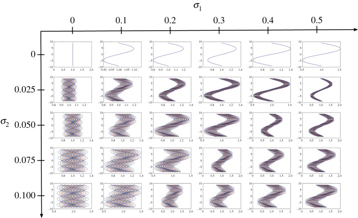
The proposed multi-fidelity modelling framework is illustrated here considering a single model in physical space and three models in probability space. The physical model returns realizations of the flow field solution produced by direct numerical simulations of equation (3.12) using the SEM. All simulations are started from a zero-velocity initial condition, and are integrated until a stable limit-cycle state is reached. This state is characterized by the well-known von Karman vortex shedding pattern in which the unsteady separation of the flow around the cylinder gives rise to a time-periodic base pressure signal. We choose three models in probability space to compute the expectation operator in equation (3.2). The highest fidelity model is probabilistic collocation on a tensor product grid (PCM) [20], the intermediate fidelity is a SG-L2 [21] and lowest fidelity model is MC integration [17]. For each model, we construct a uniform grid in the (σ1,σ2)-plane, and perform an ensemble of simulations at each grid-point according to the corresponding sampling strategy for integrating out (ξ1,ξ2) (table 3). Figure 10 illustrates the PCM samples of the inflow boundary condition for different values of (σ1,σ2). This uncertainty quantification task results to a total of 5526 Navier–Stokes simulations that were performed in parallel on one rack of IBM BG/Q (16 384 cores) with a CPU time of about 40 min.
Table 3.
Size of the uniform discretization grid in the (σ1,σ2)-plane, and number of samples per grid-point for each of the probabilistic methods employed.
| method | (σ1,σ2)-grid | samples/grid-point | total samples |
|---|---|---|---|
| PCM | 6×5 | 64 | 1920 |
| SG-L2 | 11×9 | 22 | 2178 |
| MC | 21×17 | 4 | 1428 |
Figure 10.
Modelling of the stochastic inflow: probabilistic collocation (PCM) samples of the velocity inflow profile on a uniform 6×5 (σ1,σ2)-grid. At each grid point, a total of 64 samples is used to integrate out the randomness introduced by (ξ1,ξ2) in equation (3.13). Note that σ1 controls the skewness of the inflow profile, while σ2 acts as a noise amplifier. (Online version in colour.)
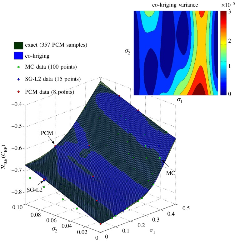
Figure 11 shows the response surface for the 0.6-superquantile risk of the base pressure coefficient , computed using a three-level recursive co-kriging. The predictive scheme is trained using 100 low-fidelity (MC), 15 intermediate fidelity (SG-L2) and only five high-fidelity (PCM) observation points in the (σ1,σ2)-plane. The accuracy of the co-kriging predictor is assessed against an ‘exact’ response surface constructed by using 357 uniformly distributed observations of the highest fidelity model (PCM), returning an error of 0.051 in the norm. More importantly, the uncertainty of the co-kriging predictor is negligible, as its variance is firmly bounded below 3×10⁻⁵. Note that if we only used a one-level kriging scheme trained on the five high-fidelity observations, the resulting is 3.536. It is evident that incorporating information from lower fidelity sources can drastically improve the accuracy of the metamodel.
Figure 11.
Response surface of the 0.6-superquantile risk of the base pressure coefficient , computed using a three-level recursive co-kriging scheme, on 100 low-fidelity (MC), 15 intermediate fidelity (SG-L2) and five high-fidelity (PCM) observation points in the (σ1,σ2)-plane. The exact surface corresponds to 357 uniformly distributed observations of the highest fidelity model (PCM). The inset plot shows the point-wise variance of the co-kriging predictor. (Online version in colour.)
4. Discussion
The scope of this work is to define a comprehensive mathematical framework that allows for the seamless integration of surrogate-based optimization and uncertainty quantification in engineering design problems. The proposed methodology targets the construction of response surfaces of complex stochastic dynamical systems by blending multiple information sources via auto-regressive stochastic modelling. We develop a general setting, under which multi-fidelity in models and multi-fidelity in probability space can coexist in tandem. A computationally efficient framework is developed using multi-level recursive co-kriging and GMRFs, resulting in very robust schemes in two- and three dimensions.
The capabilities of our implementation were tested for three different cases. In all cases, we were able to successfully exploit cross-correlations within ensembles of surrogate models and efficiently construct an accurate estimate for the response of the given stochastic system. In particular, we were able to construct the response surface and identify an optimal risk-averse design for a benchmark problem involving a short structural column with random material properties being subject to random loads. Next, we considered the regression of a random function, for which different fidelity models and information sources were available both in physical and probability spaces. An accurate representation is obtained by only using a minimal amount of expensive high-fidelity observations along with many cheap, low-quality realizations of different surrogates. The third benchmark case we considered involved evolving the Burgers equation from a random initial state and tracking the statistics of the kinetic energy of the system at a later time. Our results demonstrate how the proposed multi-fidelity framework can provide an accurate quantification of uncertainty with orders of magnitude of decrease in computational demands. Finally, we presented a realistic uncertainty quantification case for a laminar stochastic wake past a circular cylinder. For this case, we were able to obtain an accurate and reliable estimation of the response surface for the superquantile risk of the base pressure coefficient—a quantity that is known for its high sensitivity to the flow conditions.
A limiting factor of our presentation stems from the fact that all demonstrations were confined to two-dimensional problems. Although this significantly contributes towards enhancing the clarity of the presented concepts, we acknowledge that it does not establish a direct link to realistic high-dimensional design problems. To this end, the proposed framework can be extended to hypercube design spaces, in which covariance models can be similarly trained on the data through the SPDE approach, that can now be discretized using orthogonal tensor product expansion bases. This technique can provide an adequate extension to handle high-dimensional problems, however, its cost and optimality need to be carefully assessed. Our future plans will focus on evaluating the available tools and identifying an optimal strategy for addressing high-dimensionality in both the design and probability spaces.
Supplementary Material
Supplementary Material
Supplementary Material
Supplementary Material
Acknowledgements
We are thankful to Dr Lucia Parussini (Department of Mechanical Engineering, University of Trieste, Italy) for her help during the initial implementation stages of this work.
Data accessibility
The datasets supporting this article have been uploaded as part of the electronic supplementary material (ESM).
Author' contributions
P.P. developed and implemented the methods, designed and performed the numerical experiments and drafted the manuscript; D.V. conceived and supervised the design and implementation of the methods and simulations; J.O.R. provided guidance on the use of risk measures and risk-averse design and helped draft the manuscript; G.E.K. conceived and coordinated the study. All authors gave final approval for publication.
Competing interests
We declare we report no competing interests linked to this study.
Funding
P.P., D.V. and G.E.K. gratefully acknowledge support from DARPA grants nos HR0011-14-1-0060, AFOSR grant no. FA9550-12-1-0463 and the resources at the Argonne Leadership Computing Facility (ALCF), through the DOE INCITE program. J.O.R. acknowledges support from DARPA grant no. HR001-14-1-225.
References
- 1.Forrester A, Sóbester A, Keane A. 2008. Engineering design via surrogate modelling: a practical guide. New York, NY: John Wiley & Sons. [Google Scholar]
- 2.Rasmussen CE, Williams CKI. 2005. Gaussian processes for machine learning. Cambridge, MA: The MIT Press. [Google Scholar]
- 3.Hastie T, Tibshirani R, Friedman J, Hastie T, Friedman J, Tibshirani R. 2009. The elements of statistical learning. Berlin, Germany: Springer. [Google Scholar]
- 4.Cressie N. 1993. Statistics for spatial data. New York, NY: Wiley-Interscience. [Google Scholar]
- 5.Matheron G. 1963. Principles of geostatistics. Econ. Geol. 58, 1246–1266. (doi:10.2113/gsecongeo.58.8.1246) [Google Scholar]
- 6.Krige DG. 1951. A statistical approach to some mine valuation and allied problems on the Witwatersrand. Ph.D. thesis, University of the Witwatersrand. [Google Scholar]
- 7.Sacks J, Welch WJ, Mitchell TJ, Wynn HP. 1989. Design and analysis of computer experiments. Stat. Sci. 4, 409–423. (doi:10.1214/ss/1177012413) [Google Scholar]
- 8.Simpson TW, Toropov V, Balabanov V, Viana FA. 2008. Design and analysis of computer experiments in multidisciplinary design optimization: a review of how far we have come or not. In 12th AIAA/ISSMO multidisciplinary analysis and optimization conf, Victoria, BC, Canada, 10–12 September, vol. 5, pp. 10–12. Reston, VA: AIAA. [Google Scholar]
- 9.Kennedy MC, O'Hagan A. 2000. Predicting the output from a complex computer code when fast approximations are available. Biometrika 87, 1–13. (doi:10.1093/biomet/87.1.1) [Google Scholar]
- 10.Forrester AI, Sóbester A, Keane AJ. 2007. Multi-fidelity optimization via surrogate modelling. Proc. R. Soc. A 463, 3251–3269. (doi:10.1098/rspa.2007.1900) [Google Scholar]
- 11.Le Gratiet L, Garnier J. 2014. Recursive co-kriging model for design of computer experiments with multiple levels of fidelity. Int. J. Uncertain. Quantification 4, 365–386. (doi:10.1615/Int.J.UncertaintyQuantification.2014006914) [Google Scholar]
- 12.Lindgren F, Rue H, Lindström J. 2011. An explicit link between Gaussian fields and Gaussian Markov random fields: the stochastic partial differential equation approach. J. R. Stat. Soc. B 73, 423–498. (doi:10.1111/j.1467-9868.2011.00777.x) [Google Scholar]
- 13.Phadke MS. 1995. Quality engineering using robust design. Englewood Cliffs, NJ: Prentice Hall, PTR. [Google Scholar]
- 14.Seshadri P, Constantine P, Iaccarino G, Parks G. 2014. Aggressive design: a density-matching approach for optimization under uncertainty. (http://arxiv.org/abs/1409.7089)
- 15.Rockafellar RT, Royset JO. 2015. Engineering decisions under risk-averseness. ASCE-ASME J. Risk Uncertain. Eng. Syst. A 1, 04015003 (doi:10.1061/AJRUA6.0000816) [Google Scholar]
- 16.Le Gratiet L. 2013. Multi-fidelity Gaussian process regression for computer experiments. Ph.D. thesis, Université Paris-Diderot, Paris VII, France. [Google Scholar]
- 17.Binder K, Heermann D. 2010. Monte Carlo simulation in statistical physics: an introduction. Berlin, Germany: Springer Science & Business Media. [Google Scholar]
- 18.Yang X, Choi M, Lin G, Karniadakis GE. 2012. Adaptive ANOVA decomposition of stochastic incompressible and compressible flows. J. Comput. Phys. 231, 1587–1614. (doi:10.1016/j.jcp.2011.10.028) [Google Scholar]
- 19.Xiu D, Karniadakis GE. 2003. Modeling uncertainty in flow simulations via generalized polynomial chaos. J. Comput. Phys. 187, 137–167. (doi:10.1016/S0021-9991(03)00092-5) [Google Scholar]
- 20.Foo J, Karniadakis GE. 2010. Multi-element probabilistic collocation method in high dimensions. J. Comput. Phys. 229, 1536–1557. (doi:10.1016/j.jcp.2009.10.043) [Google Scholar]
- 21.Novak E, Ritter K. 1996. High dimensional integration of smooth functions over cubes. Numer. Math. 75, 79–97. (doi:10.1007/s002110050231) [Google Scholar]
- 22.Kuo FY, Sloan IH, Wasilkowski GW, Woźniakowski H. 2010. Liberating the dimension. J. Complex. 26, 422–454. (doi:10.1016/j.jco.2009.12.003) [Google Scholar]
- 23.Royset JO. 2013. On sample size control in sample average approximations for solving smooth stochastic programs. Comput. Optim. Appl. 55, 265–309. (doi:10.1007/s10589-012-9528-1) [Google Scholar]
- 24.Whittle P. 1963. Stochastic-processes in several dimensions. Bull. Int. Stat. Inst. 40, 974–994. [Google Scholar]
- 25.Rozanov YA. 1982. Markov random fields. Berlin, Germany: Springer. [Google Scholar]
- 26.Karniadakis GE, Sherwin SJ. 2005. Spectral/hp element methods for computational fluid dynamics. Oxford, UK: Oxford University Press. [Google Scholar]
- 27.Jones DR, Schonlau M, Welch WJ. 1998. Efficient global optimization of expensive black-box functions. J. Glob. Optim. 13, 455–492. (doi:10.1023/A:1008306431147) [Google Scholar]
- 28.Kuschel N, Rackwitz R. 1997. Two basic problems in reliability-based structural optimization. Math. Methods Oper. Res. 46, 309–333. (doi:10.1007/BF01194859) [Google Scholar]
Associated Data
This section collects any data citations, data availability statements, or supplementary materials included in this article.
Supplementary Materials
Data Availability Statement
The datasets supporting this article have been uploaded as part of the electronic supplementary material (ESM).


