NEURAL HETEROGENEITIES INFLUENCE ENVELOPE AND TEMPORAL CODING AT THE SENSORY PERIPHERY

Abstract

Peripheral sensory neurons respond to stimuli containing a wide range of spatio-temporal frequencies. We investigated electroreceptor neuron coding in the gymnotiform wave-type weakly electric fish Apteronotus leptorhynchus. Previous studies used low to mid temporal frequencies (<256 Hz) and showed that electroreceptor neuron responses to sensory stimuli could be almost exclusively accounted for by linear models, thereby implying a rate code. We instead used temporal frequencies up to 425 Hz, which is in the upper behaviorally relevant range for this species. We show that electroreceptors can: (A) respond up to the highest frequencies tested and (B) display strong nonlinearities in their responses to such stimuli. These nonlinearities were manifested by the fact that the responses to repeated presentations of the same stimulus were coherent at temporal frequencies outside of those contained in the stimulus waveform. Specifically, these consisted of low frequencies corresponding to the time varying contrast or envelope of the stimulus as well as higher harmonics of the frequencies contained in the stimulus. Heterogeneities in the afferent population influenced nonlinear coding as afferents with the lowest baseline firing rates tended to display the strongest nonlinear responses. To understand the link between afferent heterogeneity and nonlinear responsiveness, we used a phenomenological mathematical model of electrosensory afferents. Varying a single parameter in the model was sufficient to account for the variability seen in our experimental data and yielded a prediction: nonlinear responses to the envelope and at higher harmonics are both due to afferents with lower baseline firing rates displaying greater degrees of rectification in their responses. This prediction was verified experimentally as we found that the coherence between the half-wave rectified stimulus and the response resembled the coherence between the responses to repeated presentations of the stimulus in our dataset. This result shows that rectification cannot only give rise to responses to low frequency envelopes but also at frequencies that are higher than those contained in the stimulus. The latter result implies that information is contained in the fine temporal structure of electroreceptor afferent spike trains. Our results show that heterogeneities in peripheral neuronal populations can have dramatic consequences on the nature of the neural code.

Uncovering the mechanisms by which sensory neurons encode behaviorally relevant stimuli remains an important problem in systems neuroscience. This is complicated by the fact that sensory neurons can respond both linearly and nonlinearly to stimulation. An example of this is seen in the auditory system, where neurons will not only respond to the stimulus waveform itself, but also to its time varying contrast or envelope (e.g. Frisina, 2001). Simply speaking, the envelope can be thought of as the line that connects successive maxima in the stimulus waveform (Scharf and Buus, 1986). Psychophysical studies have shown that the information contained in the envelope waveform is sufficient for speech perception in humans (Smith et al., 2002; Zeng et al., 2005). Envelopes are also found in natural visual images and are presumably used by the brain in order to distinguish contrast-based visual contours (Grosof et al., 1993; Mareschal and Baker, 1998; Tanaka and Ohzawa, 2006). Another example of a nonlinear code consists of temporal coding where the neural response displays precision at time scales that are smaller than those contained in the stimulus waveform and has been observed in a variety of systems (Carr and Konishi, 1990; Carr, 1993; Joseph and Hyson, 1993; Johansson and Birznieks, 2004; Jones et al., 2004). The mechanisms that underlie the generation of nonlinear codes are poorly understood in general and this is particularly the case for the coding of envelopes.

Gymnotiform weakly electric fish sense distortions of their self-generated electric field (electric organ discharge, EOD) through an array of electroreceptors located on their skin surface (Zakon, 1986; Kawasaki, 2005). These distortions can be due to objects such as prey in their environment or to interference with the electric field of a conspecific. Here, we focus on the coding properties of P-type electroreceptor afferents in wavetype gymnotiform fish whose probability of firing an action potential on a given EOD cycle depends on the amplitude of the EOD, that is, they respond to amplitude modulations (AMs) of the EOD through smooth changes in firing rate (Scheich et al., 1973; Bastian, 1981a). Static nonlinearities, such as saturation and rectification, have been described for these P-units but only for stimulus intensities that are outside those found in behaviorally relevant situations (Scheich et al., 1973). Therefore, most analysis of these neurons has been performed using linear systems identification techniques (Wessel et al., 1996; Nelson et al., 1997; Kreiman et al., 2000). Recent results using information theoretic measures have confirmed the mostly linear response properties of P-units and no response to stimulus envelopes has been observed (Carlson and Kawasaki, 2006, 2008; Chacron, 2006; Middleton et al., 2006). These electroreceptor afferents make synaptic contact unto pyramidal cells within the electrosensory lateral line lobe (ELL) of the hindbrain. In contrast to primary afferents, pyramidal cells show strong nonlinear coding (Chacron, 2006; Middleton et al., 2006), which is at least partly due to the fact that these cells respond to the stimulus waveform as well as its envelope (Middleton et al., 2006).

An important caveat is that previous studies have characterized the responses of primary afferents to AM stimuli only up to a maximum temporal frequency of 256 Hz (Bastian, 1981a). While the range of AM frequencies caused in the context of electrolocation of objects is only 25 Hz, the AM frequencies experienced in communication situations can range from a few hertz up to 400 Hz with the highest frequencies occurring in male-female interactions in A. leptorhynchus (Nelson and MacIver, 1999; Zakon et al., 2002). Further, when conspecifics interact at close range, the resulting AM contrasts can be considerably higher than those used in previous work (Wessel et al., 1996; Nelson et al., 1997; Kreiman et al., 2000; Kelly et al., 2008) (G. Hupé and J.E. Lewis, personal communication).

We recorded the responses of P-type electroreceptor afferents to AM stimuli consisting of bandpass-filtered Gaussian white noise with 50 Hz bandwidth and center frequencies up to 400 Hz and for contrast up to 45%. We found that these neurons respond both to envelopes and to frequencies that are higher than those contained in the AM stimulus waveform. A combination of quantitative analysis techniques and mathematical modeling is used to provide an explanation for this result. Whereas previous studies have often assumed that peripheral electrosensory receptor neurons displayed a rate code, our results show that these can actually display strongly nonlinear responses to behaviorally relevant stimuli in the form of responses to envelopes as well as higher harmonics of the frequencies contained in the stimulus. The latter result implies that these electroreceptors use a temporal code to transmit information about the AM stimulus.

EXPERIMENTAL PROCEDURES

The weakly electric fish species Apteronotus leptorhynchus was used exclusively in this study. Fish were obtained from tropical fish dealers and acclimated to the laboratory as per published guidelines (Hitschfeld et al., 2009). Fish were immobilized by injection of 0.05 ml of tubocurarine chloride hydrate solution (5 mg/ml; SIGMA, St. Louis, MO, USA) and were artificially respirated with a constant flow of water over their gills (−10 ml/min). Water temperature was kept between 26 and 28 °C. Surgical procedures to expose the caudal lobe of the cerebellum were performed as previously described (Bastian, 1996a,b; Bastian et al., 2002; Chacron and Bastian, 2008; Krahe et al., 2008; Toporikova and Chacron, 2009). All animal care and surgical procedures were approved by McGill University’s animal care committee.

Recording

Sharp glass micropipette electrodes (50–100 MΩ) backfilled with 3 M KCl were used to record in vivo from P-type electrosensory afferent axons in the deep fiber layer of the ELL as done previously (Bastian, 1981a; Chacron et al., 2005a; Chacron, 2006). These units are easily identified as their probability of firing increases with increasing EOD amplitude (Scheich et al., 1973). The recorded potential was amplified (Duo 773 Electrometer, World Precision Instruments, Sarasota, FL, USA), and digitized (10 kHz sampling rate) using CED 1401plus hardware and Spike2 software (Cambridge Electronic Design, Cambridge, UK).

Stimulation

Under natural conditions, electric fish will experience both AMs as well as phase modulations of their own EOD. In this study, we only consider AMs, because they represent the relevant stimulus for the P-type primary afferents (Scheich et al., 1973). As the electric organ of A. leptorhynchus consists of modified spinal motoneurons, it remains functional during the neuromuscular blockade used in the experiments. The generation of our electrosensory stimuli followed established techniques (Bastian, 1981a; Bastian et al., 2002; Chacron, 2006; Krahe et al., 2008; Toporikova and Chacron, 2009). Briefly, the stimuli were EOD AMs and were produced by applying a train of sinusoidal waveforms to the fish. A single-cycle sinusoid was triggered at the zero crossing of each EOD cycle and its period was set to be slightly less than that of the EOD cycle, which ensured that the train remained synchronized to the animal’s own EOD. The AM stimuli consisted of zero-mean Gaussian white noise stimuli that were band-pass filtered (4th order Butterworth filter) between f_m − 25 Hz and f_m + 25 Hz, where f_m =100, 200, 300, or 400 Hz. These AM waveforms were multiplied with the train of single-cycle sinusoids (MT3 multiplier; Tucker-Davis Technologies, Gainesville, FL, USA). The resulting signal was isolated from ground (World Precision Instruments A395 linear stimulus isolator), passed through a step attenuator for controlling its intensity, and then applied via two electrodes located on either side of the animal (Fig. 1A, electrodes 1 and 2). Each stimulus lasted 20 s and was repeated five times for each neuron that we recorded from.

Fig. 1.

Experimental methods. (A) Schematic diagram of the experimental setup. The animal is placed in a water-filled tank and AMs of its own EOD are delivered via stimulating electrodes 1 and 2. We recorded the changes in EOD amplitude through a small dipole (3) positioned 1–2 mm lateral to the animal. (B) Example traces of the signal recorded through the dipole when the AM consisted of 75–125 Hz noise showing the amplitude-modulated EOD (black) and the AM (blue). Also shown in red is the envelope, a non-linear transformation of the AM. (C) Power spectra of the amplitude-modulated EOD (black), AM (blue) and envelope (red) showing the different frequency contents of these signals. For interpretation of the references to color in this figure legend, the reader is referred to the Web version of this article.

We measured all stimuli presented to the animal using a small dipole positioned lateral to the animal 1–2 mm away from the skin (Fig. 1A) (Bastian et al., 2002). The stimulus contrast was defined as the ratio of the standard deviation of the EOD amplitude during stimulation to the baseline EOD amplitude (i.e. the value obtained in the absence of stimulation). The dipole was located approximately at the center of the animal were the isopotential lines of the electric field are approximately parallel to the skin surface (Rasnow et al., 1993). The stimuli were calibrated to obtain contrasts of 15%, 30%, and 45%. We note that, as predicted from modeling studies (Kelly et al., 2008), such contrasts are indeed experienced under natural conditions, such as when two fish are in close proximity to one another as occurs during agonistic encounters (G. Hupé and J.E. Lewis, personal communication).

Analysis

All data analysis was performed using custom written Matlab routines (MathWorks, Natick, MA, USA). The recorded membrane potential was first high-pass filtered (100 Hz; 8th order Butterworth). Spike times were defined as the times at which this signal crossed a given threshold value from below. A binary sequence R(t) was then constructed from the spike times in the following manner: time was first discretized into bins of width dt=0.1 ms. The value of bin i was set to 1 if there was a spike at time t_j such that i*dt< t_j <(i+1)*dt and to 0 otherwise. Note that, since the bin width dt is smaller than the absolute refractory period of the neuron, there can be at most one spike time that can occur within any given bin. This binary sequence is subsequently referred to as the neural response in the text.

Linear versus nonlinear coding

The AM stimulus waveform S(t) was sampled at 10 kHz. We quantified correlations between the neural response R(t) and the AM waveform S(t) using the stimulus-response coherence C_SR(f) which is given by (Rieke et al., 1996):

$$C_{SR}(f)=\frac{{\mid P_{SR}(f)\mid }^2}{P_{SS}(f)P_{RR}(f)}$$

where P_SR(f) is the cross-spectrum between S(t) and R(t). Here, P_RR(f) and P_SS(f) are the power spectra of R(t) and S(t), respectively. The coherence ranges between 0 and 1 and quantifies the degree to which the signals S(t) and R(t) are linearly correlated at frequency f (Roddey et al., 2000). Equivalently, the coherence measures the fraction of the stimulus at frequency f that can be accurately reproduced using an optimal linear encoding model (i.e. a model which transforms the stimulus in order to obtain the response) (Roddey et al., 2000).

We also quantified the variability in the neural response R(t) to repeated presentations of the same stimulus S(t) using the response-response coherence C_RR(f). Specifically, let R₁–R₅ be the responses obtained from the five presentations of stimulus S(t), the response-response coherence C_RR(f) is then defined by (Roddey et al., 2000; Chacron, 2006):

$$C_{RR}(f)=\frac{\frac{1}{10}{\displaystyle \sum _{i=2}^5}{\displaystyle \sum _{j=1}^{i-1}}{\mid P_{R_i{R}_j}(f)\mid }^2}{P_{RR}{(f)}^2}$$

where P_RiRj(f) is the cross-spectrum between the responses R_i(t) and R_j(t). The stimulus-response coherence C_SR(f) is related to a lower bound on the amount of information that is contained in the spike train whereas the square rooted response-response coherence [C_RR(f)]^1/2 is related to an upper bound on the amount of information that is contained in the spike train (Borst and Theunissen, 1999; Marsat and Pollack, 2004; Passaglia and Troy, 2004; Chacron, 2006).

Intuitively, any trial-to-trial variability in the neural response to repeated presentations of the same stimulus will decrease the response-response coherence C_RR(f). As such, previous studies have shown that the square rooted response-response coherence [C_RR(f)]^1/2 measures the maximum possible fraction of the response at frequency f that can be accurately reproduced using an optimal encoding model, which is in general nonlinear (Roddey et al., 2000). As mentioned above, the stimulus-response coherence C_SR(f) measures the fraction of the response at frequency f that can be accurately reproduced using the optimal linear encoding model (Roddey et al., 2000). Note that, in general, we have [C_RR(f)]^1/2≥C_SR(f) as a nonlinear model can outperform a linear one. As such, the difference between the stimulus-response C_SR(f) and the square rooted response-response coherence [C_RR(f)]^1/2 quantifies the degree to which a nonlinear model might be necessary to explain the relationship between the stimulus S(t) and the response R(t) at frequency f (Roddey et al., 2000). As such, such a difference implies that there could be a nonlinear relationship between the stimulus and response. One can test and therefore gain information as to the nature of this nonlinear relationship by first applying a given nonlinear transformation to the stimulus S(t) and then computing the coherence between the transformed stimulus and the neural response R(t). If this coherence is equal to [C_RR(f)]^1/2 at frequency f, then this implies that there was indeed a nonlinear relationship between the stimulus and response at frequency f and that we have uncovered its nature. Note that such approaches have been used previously with success (Middleton et al., 2006).

Specifically, we applied two nonlinear transformations to the stimulus S(t). The first consisted of extracting the envelope E(t) in the following way. First, the Hilbert transform Ŝ(t) of S(t) was computed as:

$$\widehat{S}(t)=\frac{1}{\pi }C\left[\underset{-\infty }{\overset{\infty }{\int }}\frac{S(\tau )}{t-\tau }d\tau \right]$$

where C represents the Cauchy principal value (Zygmund, 1968). The time varying envelope E(t) was then computed as:

$$E(t)=\sqrt{S{(t)}^2+\widehat{S}{(t)}^2}$$

We then computed the stimulus-response coherence between the response R(t) and the envelope E(t), C_ER(f), as:

$$C_{ER}(f)=\frac{{\mid P_{ER}(f)\mid }^2}{P_{EE}(f)P_{RR}(f)}$$

The second nonlinear transformation consisted of rectifying the stimulus S(t) by setting the values below a given threshold equal to that threshold in order to obtain S_rect(t). In order to test whether rectification could explain the nonlinear responses of electroreceptor afferents, we then computed the stimulus-response coherence between the rectified stimulus S_rect(t) and the response R(t) as:

$$C_{\mathit{RECT}}(f)=\frac{{\mid P_{S_{\mathit{rect}}R}(f)\mid }^2}{P_{S_{\mathit{rect}}{S}_{\mathit{rect}}}(f)P_{RR}(f)}$$

where P_SrectR(f) is the cross-spectrum between the rectified stimulus S_rect(t) and the response R(t), and P_SrectSrect(f) is the power spectrum of the rectified stimulus S_rect(t).

Phase histograms

We computed phase histograms from our data in the following manner. We estimated the phase ϕ(t) from the stimulus waveform S(t) as:

$$\phi (t)=arctan\left(\frac{\widehat{S}(t)}{S(t)}\right)$$

and then built histograms of the phase values corresponding to the spike times.

Segregating envelope responsive and non-envelope responsive cells

To segregate our data into envelope responsive (ER) and non-envelope responsive (NER) cells, we focused on the envelope-response coherence C_ER(f) for the 75–125 Hz stimulus because envelope coding was maximal for this frequency range. For each neuron we then took the maximum value of C_ER(f) and averaged it across the population for each contrast. The average values, <C_ER(f)≥0.14 (15% contrast), 0.23 (30%) and 0.29 (45%) were used as thresholds. Neurons for which the peak value of C_ER(f) was above the threshold for at least one contrast were tagged as ER and the remaining neurons as NER. Note that all ER neurons except one had all three peak values greater than average. Using this criterion we obtained 21 (43%) ER neurons and 28 (57%) NER neurons.

Input-output transfer function

We characterized the input-output transfer function of electroreceptors in the following manner. The response R(t) was first filtered using a 15 point Kaiser filter in order to obtain the time dependent firing rate. Previous studies have shown that such a filter provides a good estimate of modulations in the time varying firing rate of neurons provided that the mean firing rate is high (Cherif et al., 2008), which is the case here as primary afferents have firing rates greater than 150 Hz (Gussin et al., 2007). The stimulus waveform S(t) was aligned to the time dependent firing rate and transformed according to:

$$S_{\mathit{norm}}(t)=\frac{S(t)-min[S(t)]}{max[S(t)]-min[S(t)]}$$

where min[S(t)] and max[S(t)] are the minimum and maximum values of S(t), respectively. The normalized stimulus S_norm(t) thus ranges between 0 and 1. We then plotted the time dependent firing rate as a function of this normalized stimulus to obtain the input-output transfer function. This transfer function was then fitted with a sigmoid given by:

$$\mathit{SIG}(x)=\frac{r_{max}}{1+exp\left(-\frac{x-S_{1/2}}{k}\right)}$$

where r_max is the maximum firing rate, S_1/2 is the inflexion point defined by:

$$\mathit{SIG}(S_{1/2})=\frac{r_{max}}{2}$$

and k is proportional to the inverse of the slope of the sigmoid at the inflexion point S_1/2.

Modeling

In order to gain greater understanding as to what causes a neuron to respond to the envelope, we used a previously described leaky integrate and fire model with dynamic threshold (LIFDT) (Chacron et al., 2000, 2001a, 2003b) with a burst current (Chacron et al., 2001b, 2004). The model is described by the following differential equations:

$$\begin{array}{c}{V}^Y=-\frac{V}{{\tau }_v}+\frac{I_{\mathit{stim}}(t)}{{\tau }_v}\\ {\theta }^Y=\frac{{\theta }_0-\theta }{{\tau }_{\theta }}\\ I_{\mathit{stim}}(t)=(S(t)+A_0)sin(2\pi f_{\mathit{EOD}}t)\mathrm{\Theta }[S(t)+A_0]\mathrm{\Theta }[sin(2\pi f_{\mathit{EOD}}t)](1+\sigma \xi (t))+I_b(t)+I_{\mathit{bias}}\\ I_b^Y(t)=-\frac{I_b}{{\tau }_b}+\mathrm{\Delta }{I}_b\sum _{i=1}^{N(t)}\delta (t-d-t_i)\end{array}$$

where v is the membrane potential, τ_v is the membrane time constant, θ is the threshold, and τ_θ is the threshold time constant. Here θ₀ is the threshold equilibrium value. When v is equal to θ, a spike is said to occur and v is immediately reset to 0 and remains equal to 0 for the duration of the absolute refractory period T_r. Further, θ is incremented by a fixed amount Δθ. I_stim(t) is the total input current consisting of the modulated EOD waveform, a bias current I_bias, and a bursting current I_b(t). σ ξ(t) is a Gaussian white noise process with zero mean and standard deviation σ, f_EOD is the EOD frequency, and Θ(t) is the Heaviside function defined by:

$$\begin{array}{lll}\mathrm{\Theta }(t)=1\hfill & if\hfill & t\ge 0\hfill \\ \mathrm{\Theta }(t)=0\hfill & if\hfill & t<0\hfill \end{array}$$

The additive current I_b(t) controls the amount of bursting in the model. This current decays exponentially with time constant τ_b and is incremented by a fixed amount ΔI_b after a time delay d following each spike time t_i. We note that a full biophysical justification of this current and of the model in general can be found in (Chacron et al., 2001a,b; Chacron et al., 2004). Previous studies have also shown that this model could reproduce experimental data from electroreceptor afferents with good accuracy (Chacron et al., 2001a,b, 2004). The model was simulated numerically using an Euler-Maruyama algorithm (Kloeden and Platen, 1999) with integration time step dt=0.025 ms. Parameter values used are given in Table 1.

Table 1.

Parameter values used in numerical simulations of our model are similar to those used in previous studies (Chacron et al., 2001b, 2004)

τv	τθ	A0	fEOD	ξ	θ0	Δθ	ΔIb	d	tb
0.8 ms	7.75 ms	0.06	760 Hz	0.1	0.03	0.01	0.07	0	1 ms

We generated experimentally observed heterogeneities in the baseline firing rate by varying the parameter I_bias between 0 and 0.315 (with A₀ fixed at 0.06) which led to baseline firing rates between 149.4 and 450.4 Hz in our model. This range is in good agreement with the one obtained from experimental observations (Xu et al., 1996; Gussin et al., 2007). We note that similar results could be obtained by varying A₀ between 0.06 and 0.131 with I_bias=0 (data not shown).

RESULTS

We recorded from n=49 receptor afferents in nine fish (mean EOD frequency 761±64 Hz). AMs of the animal’s own EOD were delivered via two transverse electrodes in the “global” stimulation geometry (Bastian et al., 2002; Chacron, 2006; Krahe et al., 2008; Toporikova and Chacron, 2009; Avila-Akerberg et al., 2010) (Fig. 1A). We chose the AM stimuli (Fig. 1B, blue) to have temporal frequency content between f_m − 25 Hz and f_m +25 Hz, where f_m = 100, 200, 300, or 400 Hz. We computed the instantaneous amplitude, or envelope (Fig. 1B, red) of the AM using the Hilbert transform as described in the methods. We note that all the stimuli used in this study have an envelope that contains temporal frequencies within the range 0–50 Hz (Fig. 1C, red).

Electroreceptor afferents display nonlinear responses to high frequency EOD AMs

Afferents responded strongly to the AM waveform as shown by a representative example (Fig. 2). The action potential times tended to occur most frequently during the stimulus downstrokes and only rarely during the stimulus upstrokes as seen for five repetitions of the same AM stimulus waveform (Fig. 2A, dots). While this may seem surprising at first, we note that this is due to the axonal transmission delay of ~5 ms between the surface of the skin and the recording site (Nelson et al., 1997; Chacron et al., 2003b). A qualitative inspection of Fig. 2 showed that this example afferent responded to both the high frequency (75–125 Hz) of the AM (Fig. 2A) and the lower frequency (1–50 Hz) of the envelope (Fig. 2B) extracted from the AM using the Hilbert transform. This is most easily seen by plotting the responses as well as the envelope and AM stimulus waveforms on a longer time scale where it is seen that the probability to fire action potentials increased for larger values of the envelope (Fig. 2B).

Fig. 2.

Electroreceptor afferents respond to the AM itself as well as its envelope. (A) AM waveform (75–125 Hz, 30% contrast, solid black) and raster plot showing the spike times (bars) obtained in response to five repeated presentations of this AM stimulus. The unit fires action potentials for a narrow range of AM phases. The envelope waveform (dashed) is also shown (dashed gray). (B) The responses of this same electroreceptor to the same AM waveform are shown for a larger length of time. This unit displayed increases in firing rate as a function of increases in envelope amplitude. Note that the time scale bar differs between panels (A, B) and that the envelope and AM signals were slightly offset with respect to one another in both panels for display purposes.

Quantifying linear and non-linear electroreceptor afferent responses

We quantified nonlinear responses across our dataset by computing the coherence between the AM and the neural response, C_SR(f), as well as the coherence between the envelope and neural response, C_ER(f). These quantities were then compared to the square root of the response-response coherence between spike trains obtained from repeated presentations of the same stimulus, [C_RR(f)]^1/2. The coherence measures the strength of correlations between the stimulus and the response and ranges between 0 (no correlation) and 1 (maximum correlation). While C_SR(f) quantifies the fraction of the stimulus at frequency f that can be correctly estimated by an optimal linear encoding model, [C_RR(f)]^1/2 quantifies the maximum fraction of the stimulus at frequency f that could be correctly estimated by an optimal encoding model (Roddey et al., 2000). Any difference between C_SR(f) and [C_RR(f)]^1/2 indicates that a nonlinear encoding model could potentially outperform the optimal linear encoding model. Such differences can occur if the neuron is responding to nonlinear transformations of the stimulus (Middleton et al., 2006) (see Experimental procedures).

In order to elucidate whether electroreceptor afferents responded to nonlinear transformations of the AM waveform, we compared the envelope response coherence, C_ER(f), to [C_RR(f)]^1/2. Fig. 3 shows [C_RR(f)]^1/2 (dashed), C_SR(f) (grey), and C_ER(f) (black) for a representative afferent for AM bandwidths of 75–125 Hz (Fig. 3A), 175–225 Hz (Fig. 3B), 275–325 Hz (Fig. 3C), and 375–425 Hz (Fig. 3D). This unit displayed a strong response to the 75–125 Hz AM stimulus as quantified by a peak stimulus response coherence that was greater than 0.8. The peak value of the stimulus-response coherence C_SR(f) decreased for higher frequency stimuli (Fig. 3, compare grey curves) but remained above 0.4. The square root of the response-response coherence, [C_RR(f)]^1/2, was almost equal to the stimulus-response coherence C_SR(f) over the AM stimulus’ temporal frequency content (Fig. 3, compare dash and grey curves). However, [C_RR(f)]^1/2 displayed non-zero values at frequencies different than those contained in the AM. In particular, it displayed peaks at low temporal frequencies (~10 Hz), which were most pronounced for 75–125 Hz noise stimuli (Fig. 3). This implies that, at these frequencies, the neuron might be responding to a nonlinear transformation of the AM. As previous studies have shown that these frequencies are contained within the envelope waveform (Middleton et al., 2006), we computed the coherence between the envelope and spike train, C_ER(f). We found that C_ER(f) was non-zero at low frequencies and furthermore was approximately equal to [C_RR(f)]^1/2 for these frequencies (compare black and dashed curves in Fig. 3A–D), indicating that this electroreceptor was indeed responding to the envelope. This electroreceptor afferent also displayed a large [C_RR(f)]^1/2 at the harmonic of the AM (2*f_m) which is not contained in the stimulus waveform itself implying that this electroreceptor might be responding to a nonlinear transformation of the stimulus at these frequencies which are not associated with the envelope. We will return to this important point later.

Fig. 3.

Quantifying afferent responses to AM stimuli of different frequency content. Coherence curves between the response of the same neuron as in Fig. 2 and the AM C_SR(f) (grey), envelope C_ER(f) (black) as well as the square rooted response-response coherence [C_RR(f)]^1/2 (dashed). These curves were calculated for 75–125 Hz (A), 175–225 Hz (B), 275–325 Hz (C) and 375–425 Hz (D) AM stimuli and for 30% contrast.

We next quantified the responses of electroreceptor afferents using coherence measures across our dataset (Fig. 4). The population-averaged values for the stimulus-response (Fig. 4A), response-response (Fig. 4B) and envelope-response (Fig. 4C) coherences are shown for 15% (white), 30% (grey) and 45% (black) contrast. Electroreceptor afferents responded best to the lowest stimulus frequencies (75–125 Hz) and their coherence values decreased with increasing stimulus frequency content for C_SR(f) and C_ER(f). The stimulus-response coherence C_SR(f) was still surprisingly high with values above 0.4 for 375–425 Hz (Fig. 4A) indicating that, on average, receptor afferents can indeed respond to the highest AM frequencies that can occur under natural conditions in A. leptorhynchus. Our results show that the envelope-response coherence C_ER(f) decreased with increasing mean frequency of stimulation (Fig. 4C). Furthermore, the square rooted response-response coherence [C_RR(f)]^1/2 decreased to values that were approximately equal to those of the stimulus-response coherence C_SR(f) for high stimulation frequencies (compare Fig. 3A, D). This implies that correlations between the AM stimulus and the neural response were largely linear in nature at these frequencies (compare Fig. 4A, B). The stimulus-response coherence C_SR(f) increased in value with increasing stimulus contrast but at a lower rate than the envelope-response coherence C_ER(f) (compare Fig. 4A, C). This indicates that, as stimulus contrast increases, an optimal nonlinear encoding model could capture a greater percentage of the information transmitted about the stimulus. This is similar to what is seen in other systems (Roddey et al., 2000).

Fig. 4.

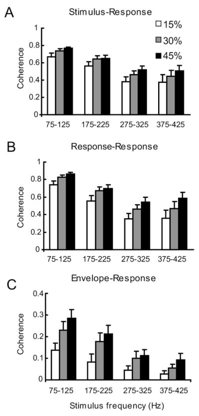
Summary of population-averaged afferent responses to AM stimuli of different contrasts (15%, 30%, and 43%) and frequency bandwidths (75–125, 175–225, 275–325, 375–425 Hz). (A) Population-averaged peak values for the stimulus-response coherence C_SR(f). (B) Population-averaged peak values for the square rooted response-response coherence [C_RR(f)]^1/2. (C) Population-averaged peak values for the envelope-response coherence C_ER(f).

Nonlinear responses and baseline firing statistics

Previous studies have shown that electroreceptor afferents display large heterogeneities in their baseline (i.e. in the absence of AMs) firing rate (Xu et al., 1996; Nelson et al., 1997; Chacron et al., 2005a; Gussin et al., 2007). Therefore, we investigated whether these heterogeneities were correlated with nonlinear responses in electroreceptor afferents.

Our results show that, while the maximum value of the stimulus-response coherence C_SR(f) was not significantly correlated with the baseline firing rate (Fig. 5A; r=−0.063; P=0.8), the maximum value of the envelope-response coherence C_ER(f) was strongly negatively correlated with the firing rate (r=−0.68; P<0.005) for 30% contrast and 75–125 Hz stimuli (Fig. 5B). In fact, we observed a strong correlation between the baseline firing rate and the maximum value of the envelope-response coherence for most stimulus frequency ranges and contrasts used in this study. The only notable exception is for high frequency stimulation (375–425 Hz) for which afferents generally do not respond well to the envelope except for the highest contrasts (Fig. 4C). These correlation coefficients are shown in Table 2.

Fig. 5.

Effects of electroreceptor afferent heterogeneities on their responses to AM stimuli. (A) The stimulus-response coherence C_SR(f) was independent of the baseline firing rate (i.e. in the absence of an AM). (B) The envelope-response coherence C_ER(f) was strongly negatively correlated with the baseline firing rate (r=−0.68; P<0.005). (C) The envelope-response coherence C_ER(f) and the square rooted response-response coherence [C_RR(f)]^1/2 evaluated at the first harmonic of the mean frequency contained in the stimulus waveform (i.e. f=200 Hz) were positively correlated (r=0.88; P<0.005). (D) Population-averaged baseline firing rates for envelope responsive (ER, black) and for non-envelope responsive (NER, gray) afferents. (E) Population-averaged coefficient of variation (CV) values for envelope responsive (ER, black) and for non-envelope responsive (NER, gray) afferents. * indicates statistical significance at the P = 0.05 levels using a Wilcoxon ranksum test.

Table 2.

Correlation coefficients between the baseline firing rate and the maximum of the envelope-response coherence obtained for the different stimulus frequency ranges and contrasts used in this study

	75–125 Hz	175–225 Hz	275–325 Hz	375–425 Hz
15%	r=−0.62; P=0.001	r=−0.58; P=0.008	r=−0.44; P=0.042	r=−0.04; P=0.915
30%	r=−0.68; P<0.001	r=−0.51; P=0.001	r=−0.44; P=0.007	r=−0.07; P=0.813
45%	r=−0.46; P=0.003	r=−0.40; P=0.003	r=−0.42; P=0.011	r=−0.59; P=0.026

It is possible that some of the heterogeneities reported in terms of envelope coding might be due to differences in the EOD frequency. While there was a small but significant positive correlation between the baseline firing rate and the EOD frequency (r=0.3032, P=0.03, n=49), normalizing the baseline firing rate of each electroreceptor by the animal’s EOD frequency (i.e. normalizing time to be in units of EOD cycles) did not qualitatively affect the significance of the correlation coefficients reported in Table 2 (data not shown). This suggests that the differences in EOD frequency cannot explain the heterogeneity of envelope responses observed across our dataset.

Finally, the maximum value of the envelope-response coherence was strongly positively correlated with the value of the square-rooted response-response coherence evaluated at f=2*f_m (Fig. 5C, r=0.88; P<0.005), implying that the responses to the envelope and the coherence between responses at higher harmonics of the frequencies contained in the stimulus might be caused by the same nonlinearity.

In order to better understand how heterogeneities in firing rate can influence nonlinear coding and thus gain insight as to the nature of the mechanism that enables nonlinear coding in electroreceptors, we divided our dataset into envelope responsive and non-envelope responsive neurons as described in the experimental procedures (see Fig. 5B for a graphical representation of the division at 30% contrast). Out of the 49 electroreceptors in our dataset, 21 (~43%) were classified as envelope responsive while the remaining 28 (~57%) were classified as non-envelope responsive. We found that envelope responsive neurons had significantly lower baseline firing rates than non-envelope responsive neurons (Fig. 5D; Wilcoxon ranksum test; P<0.001; df=48), which is expected from the strong negative correlation that was observed between the maximum values of the envelope response coherence and the baseline firing rate (Fig. 5B). Envelope responsive neurons were also found to display more variability than non-envelope responsive neurons as quantified by the coefficient of variation (CV) of the interspike intervals (ISIs; Fig. 5E; Wilcoxon ranksum test; P=0.0158; df=48). Because units with low firing rates have a greater tendency to display rectification, we hypothesized that nonlinear coding in afferents is due to rectification. Thus, we hypothesized that the coherence between responses at higher frequencies are due to the fact that the electroreceptor neurons are responding to a nonlinear transformation of the AM stimulus, rectification, and that rectification can explain the observed response to the envelope.

Modeling electroreceptor afferent responses to AM stimuli

We investigated the potential role of rectification in explaining the experimentally observed nonlinear responses of electroreceptors by using a phenomenological leaky integrate-and-fire with dynamic threshold model (LIFDT; Fig. 6A). Previous studies have provided a full biophysical justification for this model and have shown that it can reproduce both the experimentally observed heterogeneities in the baseline firing statistics of primary electrosensory afferents (Chacron et al., 2000, 2001b, 2004) as well as the experimentally observed responses to sensory input (Chacron et al., 2005b; Chacron, 2006).

Fig. 6.

Modeling linear and nonlinear afferent responses to sensory stimulation. (A) Example membrane potential (V, black), threshold (Θ, gray) and stimulus (AM, dashed) from the model. Spiking occurs when the membrane potential crosses the threshold from below, at which time voltage is reset to zero. Note that we were using 30% contrast. (B) The stimulus-response coherence C_SR(f) as a function of the firing rate of the model (dashed) was comparable to that obtained from our experimental data (solid). (C) The envelope-response coherence C_ER(f) as a function of firing rate decreased with increasing firing rate of the model neuron (dashed) similar to our experimental data (solid). (D) The square rooted response-response coherence [C_RR(f)]^1/2 evaluated at 200 Hz (i.e. the first harmonic of the mean frequency contained in the stimulus waveform) decreases as a function of increasing firing rate in the model (dashed), which is similar to our experimental data (solid).

We first applied AM stimuli to the model and found that it could qualitatively reproduce the results seen experimentally. Indeed, the stimulus-response coherence C_SR(f) was independent of the firing rate (Fig. 6B, dashed line). Moreover, the envelope-response coherence C_ER(f) decreased as a function of increasing firing rate (Fig. 6C dashed lines). We further observed that the value of the square rooted response-response coherence at the first harmonic (200 Hz) also decreased as a function of increasing firing rate as observed in the data (Fig. 6D).

We next tested whether rectification could account for the responses displayed by the model. In order to do so, we computed the stimulus response coherence of our model neuron with a stimulus that was rectified using different thresholds while keeping other parameters in the model fixed (Fig. 7A). Plotting the power spectra of these rectified waveforms revealed that they contained power not only at low frequencies associated with the envelope but also at frequencies that were twice those contained in the AM stimulus waveform (Fig. 7B). We next computed the coherence between the rectified stimulus waveform and the neural response, C_RECT(f). Our results show that C_RECT(f) had a similar profile to that of the square-rooted response-response coherence [C_RR(f)]^1/2 (Fig. 7C). Moreover, it is seen that the magnitude of the response at the envelope frequencies and at the first harmonic are maximal when the rectification threshold is equal to the mean of the stimulus waveform (i.e. when the stimulus is half-wave rectified) (Fig. 7D). Finally, we observed that the encoding of frequencies that were contained in the original stimulus waveform decreased for positive levels of rectification (Fig. 7D).

Fig. 7.

Rectification as a mechanism for generating nonlinear responses to sensory stimulation. (A) Time series of the AM stimulus waveform with different levels of half wave rectification. The values of the stimulus that were below the rectification threshold were set to the value of the threshold. (B) Power spectra associated with the stimulus rectification in (A). (C) Stimulus response coherence between the model neuron response for 75–125 Hz stimulation and the rectified AM C_RECT(f) for different levels of rectification shown in (A). This was obtained for a fixed value of the current I_bias corresponding to a representative firing rate (FR) of 150 Hz. (D) The coherence between the response and the rectified stimulus waveform C_RECT(f) was evaluated at frequencies corresponding to the envelope (20 Hz, red), AM (100 Hz, blue) and to the first harmonic (200 Hz, green) as a function of the level of rectification for a fixed value of I_bias=0 corresponding to a mean firing rate of 150 Hz. (E) The coherence between the response and the rectified stimulus waveform was evaluated at frequencies corresponding to the envelope (20 Hz, red), AM (100 Hz, blue) and to the first harmonic (200 Hz, green) as a function of the neuron’s firing rate (which was varied by changing the value of the parameter I_bias in the model between 0 and 0.0315) for a fixed level of rectification of zero. For interpretation of the references to color in this figure legend, the reader is referred to the Web version of this article.

These results show that rectification of the stimulus waveform is the nature of the nonlinear transformation being performed by our electroreceptor neuron model and implies that its response contains information at frequencies that are higher than those contained in the stimulus waveform. Equivalently, this implies that information is contained in the response at time scales that are shorter than those contained in the stimulus, which is by definition a temporal code (Theunissen and Miller, 1995; Dayan and Abbott, 2001; Jones et al., 2004; Sadeghi et al., 2007).

We then tested whether changes in the baseline firing rate brought about by changing the value of the parameter I_bias could account for the differences in nonlinear coding seen in our experimental data. We computed the stimulus-response coherence between the model’s output and the half-wave rectified stimulus for different values of I_bias. Our results show that the coherence values for frequency ranges corresponding to the envelope, stimulus waveform, and first harmonic followed trends as a function of firing rate that were qualitatively similar to those found for the experimental data (compare Figs. 6B–D and 7E).

Our model thus predicts that rectification can lead to the experimentally observed nonlinear responses in electroreceptor afferents, that information is contained in the fine structure of their spike trains, and that changes in the baseline firing rate can account for the observed heterogeneities in nonlinear coding.

Verifying the model’s prediction

In order to verify our model’s prediction that envelope responsive neurons display greater levels of rectification than non-envelope responsive neurons, we filtered the data spike trains to obtain an estimate of the time dependent firing rate and superimposed the original stimulus waveform that was time shifted by 5 ms to account for axonal transmission delays (see above) (Fig. 8A). It is seen that this particular neuron only fired action potentials when the stimulus was positive and not when the stimulus was negative, thereby strongly suggesting that this neuron was implementing half-wave rectification (Fig. 8A). We next computed the stimulus-response coherence between the half-wave rectified stimulus and the neural response C_RECT(f) and compared it to the square rooted response-response coherence [C_RR(f)]^1/2 from this particular neuron. It is seen that both quantities agree qualitatively over the frequency range (Fig. 8B, compare solid black and dashed black curves). This further supports our hypothesis that this neuron is implementing half-wave rectification. An example non-envelope responsive neuron did not show coherence peaks at envelope and harmonic frequencies, for either the square rooted response-response coherence [C_RR(f)]^1/2 or coherence between the response and the half-wave rectified stimulus C_RECT(f) (Fig. 8B, compare solid gray and dashed gray curves).

Fig. 8.

Verifying the model’s prediction. (A) Instantaneous firing rate (solid black) and stimulus (dashed) time series from an example afferent. The spike times are also shown (dots). (B) Left: Stimulus-response coherence between the half-wave rectified stimulus and the response C_RECT(f) (solid) and the square rooted response-response coherence [C_RR(f)]^1/2 (dashed), for example, envelope responsive (black) and non-envelope responsive (gray) afferents. Right: Population averages of the coherence between the half-wave rectified stimulus and the response C_RECT(f) evaluated at f=200 Hz for envelope responsive (black) and non-envelope responsive (grey) neurons. (C) The average firing rate is plotted against the normalized stimulus amplitude (hollow circles) with the standard error bars (gray) to obtain the input-output function. These data were fitted with a sigmoid function (solid black). Also shown are the sigmoid function’s inflection point S_1/2, maximum value r_max., and inverse slope at the inflection point k. (D–F) Population-averaged sigmoid fits for ER and NER afferents show differences in the position of their inflection points S_1/2. Insets: S_1/2 is larger for ER neurons. These data are shown for 75–125 Hz AM frequency content and for 15%, 30% and 45% contrast, respectively. (G) Left: Phase histograms from an example ER afferent (black) and NER afferent (gray). It is seen that the ER afferent displays greater rectification. Right: Population-averaged values of rectification were larger for ER neurons than for NER neurons. The rectification values were defined as the percent of bins for which the count was less than 30% of the mean bin count.

We then tested whether the envelope responsive neurons in our dataset displayed more rectification than the non-envelope responsive ones. The value of the stimulus-response coherence C_RECT(f) computed between the half-wave rectified stimulus and the response evaluated at 200 Hz was significantly higher for envelope-responsive neurons than for non-envelope responsive ones (P<0.001, Wilxocon ranksum test, n=35) indicating that half-wave rectification better accounts for the responses of envelope-responsive neurons (Fig. 8B).

We next plotted the neuron’s firing rate from Fig. 8A as a function of the corresponding normalized stimulus amplitude to obtain an input-output transfer function similar to what has been done previously (Gussin et al., 2007). We fitted a sigmoid function to the resulting frequency-versus-amplitude curve. This sigmoid was characterized by three parameters: the peak firing rate r_max, the inflection point S_1/2, and k which is proportional to the inverse slope at S_1/2 (Fig. 8C). Overall, we found that sigmoid fits to the input transfer functions of envelope responsive (black curve) and non-envelope responsive neurons (grey curve) differed mainly in the position of their inflection points S_1/2 for 15% (Fig. 8D), 30% (Fig. 8E), and 45% (Fig. 8F) contrasts. These differences were significant in all cases (Fig. 8D–F (insets); Wilcoxon ranksum tests; P<0.005 in all cases). Because the slopes of the input-output transfer functions were similar for both envelope responsive and non-envelope responsive neurons, the higher values of the inflection point S_1/2 observed for envelope-responsive neurons indicate that these display a greater tendency for rectification. Finally, we computed phase histograms of envelope-responsive and non-envelope responsive neurons. For a linear system, we would expect the phase histogram to vary smoothly as a function of the stimulus. In contrast, rectification is manifested in a low count over a range of phase values. Phase histograms computed from example envelope responsive and non-envelope responsive neurons show that the number of bins whose count is below a threshold value is higher for the envelope-responsive neuron (Fig. 8G). We defined a rectification index as the percentage of bins whose counts were below 30% of the mean bin count. This rectification index was significantly larger for envelope responsive neurons than for non-envelope responsive neurons (Fig. 8G, inset; Wilcoxon rank-sum test; P<0.005). The results from all these analyses suggest that rectification accounts for the nonlinear responses seen in electroreceptor afferents. We therefore conclude that rectification is most likely responsible for the nonlinear responses seen experimentally and that rectification is, as expected, more prominent in afferents with low baseline firing rates.

DISCUSSION

We have studied the responses of P-type electroreceptor afferents to high frequency AM stimulation. Our results show that these neurons can display strong responses to temporal AM frequencies up to 425 Hz that were nonlinear for a large fraction of neurons in our dataset. These nonlinearities in the response were shown to occur because electroreceptor afferents responded to a nonlinear transformation of the AM stimulus that gave rise to responses that were coherent at low temporal frequencies associated with the envelope and at higher harmonics of the frequencies contained in the AM waveform. We further showed that the neural response of some afferents was coherent with the envelope of the AM waveform. Since the magnitude of this envelope response was strongly positively correlated with response coherence measured at higher harmonics, we hypothesized that they were due to the same mechanism. In order to understand the nature of this mechanism, we partitioned our data into envelope responsive and non-envelope responsive cells and compared their properties. We found that envelope responsive neurons tended to have lower baseline firing rates than non-envelope responsive neurons. Based on a phenomenological model of electroreceptor afferent activity, we predicted that rectification could account for both the envelope response as well as the response coherence seen at higher harmonics. We then tested our modeling prediction experimentally by performing a rectification operation on the AM waveform and computing the coherence between the resulting rectified stimulus and the neural response. As this coherence was non-zero both for low frequencies associated with the envelope and at higher harmonics of the frequencies contained in the AM waveform, we concluded that rectification could indeed account both for envelope coding as well as the coherence between responses seen at higher frequencies. Moreover, this result showed that information about the stimulus is present at frequencies higher than those contained in the stimulus waveform itself. This implies that information is present at time scales that are shorter than those contained in the stimulus, which is indicative of a temporal code. Finally, we found that nonlinear coding in electroreceptors was strongly correlated with a tendency to display rectification in units with lower baseline firing rates.

Electroreceptor afferents respond to high frequency AM stimuli

Our study shows for the first time that individual electroreceptor afferents can detect AMs whose temporal frequency content can be as high as 425 Hz. This is contrary to previous studies that have shown that the responses of individual electroreceptors can start to decline for frequencies as low as 100 Hz (Bastian, 1981a; Chacron et al., 2005a). We note that Bastian (1981a) recorded from electroreceptors in A. albifrons whereas we recorded from electroreceptors in A. leptorhynchus and that this might account for differences between our results and his. However, it is most likely that the differences between our results and previous studies are due to the fact that the stimuli and contrasts used here were different than those used in those studies. Indeed, unlike previous studies, we used higher contrasts and stimuli with narrow frequency ranges.

Amplitude modulations in this frequency range can occur during interactions between males and females whose EOD frequencies can differ by as much as 400 Hz creating beats at that frequency in A. leptorhynchus. The information about high frequency AMs is most likely transmitted to higher order neurons as behavioral studies have shown that A. leptorhynchus responds to these stimuli (Engler and Zupanc, 2001). We note that A. leptorhynchus is not the only species of weakly electric fish that experiences AMs with such high frequency content. Indeed, both Eigenmannia virescens and A. albifrons can experience AMs with frequency content as high as 500 Hz (Scheich and Bullock, 1974; Tan et al., 2005). It is likely that the nonlinear coding present in the electroreceptors of A. leptorhynchus would also be present in these species. Further studies are necessary to verify this hypothesis and are beyond the scope of this paper.

Nonlinear coding in the peripheral electrosensory system

Electroreceptor afferents have traditionally been assumed to transmit information through a rate code as it was thought that their time dependent firing rate carried all the information about variations in EOD amplitude (Scheich et al., 1973; Bastian, 1981a,b; Gussin et al., 2007). As such, they have traditionally been characterized using linear systems identification techniques (Scheich et al., 1973; Bastian, 1981a; Wessel et al., 1996; Kreiman et al., 2000; Benda et al., 2005). While the presence of static nonlinearities, such as rectification and saturation, has been shown previously, they were only described for constant-amplitude stimuli at intensities outside of the physiological range (Scheich et al., 1973). More recent studies found mostly linear coding of AMs for contrasts of 10–20% (Chacron, 2006; Gussin et al., 2007). In contrast, we have shown that a large proportion of electroreceptors displayed significant nonlinear responses for contrasts as low as 15%. This apparent discrepancy is most likely due to the lower temporal frequencies used in the earlier studies (up to 50 Hz in Gussin et al. (2007) and up to 120 Hz in Chacron (2006)). Electroreceptor afferents have been shown to display stronger responses to stimuli with higher temporal frequency content (Nelson et al., 1997; Kreiman et al., 2000; Chacron et al., 2005a). High-frequency stimuli as used in the present study are thus more likely to cause nonlinearities in the response, such as rectification. Further, we note that a modeling study predicted that electroreceptor afferents might display responses to the envelope (Longtin et al., 2008). Our results have shown that there was a strong negative correlation between the baseline firing rate and the magnitude of the envelope response, thereby suggesting that the former is a strong contributor to determining whether a given electroreceptor afferent responds to the envelope. We note however that other sources might also be contributing to nonlinear coding in electroreceptors and that further studies are necessary to elucidate their nature.

We found that electroreceptor afferents with the highest firing rates were the least likely to display nonlinear coding. This is surprising as these afferents should be the most likely to show firing rate saturation which would lead to nonlinear coding. Indeed, previous studies have shown that sufficiently intense stimulation will elicit saturation (Scheich et al., 1973; Gussin et al., 2007). Yet, we did not observe any direct consequence of saturation using high frequency AM stimuli with contrasts as high as 45%. One possible explanation for this discrepancy is that our stimuli were not sufficiently strong to elicit saturation. This was, however, not the case as most of our neurons displayed strong bursting (i.e. firing on consecutive EOD cycles), which corresponds to saturation because P-units can fire at most one spike per EOD cycle (Scheich et al., 1973). Further studies are needed to fully understand why rectification plays a much greater role than saturation in eliciting nonlinear responses in peripheral electrosensory neurons.

We have also shown that the precision of spike timing in electroreceptor afferent spike trains exceeded that present in our stimuli, thereby showing that they could encode information in the timing of action potentials. By definition (Theunissen and Miller, 1995; Dayan and Abbott, 2001), our results have thus shown the presence of a timing code in electroreceptors and furthermore shown that this code was due to rectification in the response of some of these afferents to the stimuli used in this study. This result agrees with the growing amount of evidence that spike timing codes might be used as early as the sensory periphery in the somatosensory (Johansson and Birznieks, 2004) as well as vestibular (Sadeghi et al., 2007) systems. An important question is then whether information that is carried in the spike timing of electroreceptors is actually decoded by their postsynaptic targets: pyramidal cells within the ELL. Actual recordings from ELL pyramidal cells using stimuli similar to the ones used here are necessary to answer this question and are beyond the scope of this paper. We note however that our results in no way show that envelope coding by electroreceptors requires precise spike timing and are thus compatible with previous modeling results showing rate coding for envelopes in a model neuron (Middleton et al., 2007). While it could be argued that the response to higher harmonics that we observed is an artefact of the rectification displayed by some electroreceptors and might not carry any behavioral relevance, a growing amount of evidence suggests that this is not the case. Indeed, some species take into account the higher harmonics contained in a call when choosing their mate (Bodnar, 1996; Hennig, 2009) while insects can reliably track contrast-based motion patterns (Theobald et al., 2008). Further studies are needed to elucidate these important questions in the electrosensory system.

Multiple mechanisms for generating an envelope response in the electrosensory system

A previous study has shown that pyramidal cells in the ELL responded to the envelope of time varying 40–60 Hz AM stimuli for 12.5% contrast whereas receptor afferents did not (Middleton et al., 2006). This study proposed that the envelope response originated from an inhibitory ELL interneuron, the ovoid cell (Middleton et al., 2006). Our results show that envelope responses can be generated already in the primary electroreceptor afferents. While it remains to be shown if ELL pyramidal neurons display envelope responses to the stimuli used in the present study, this is likely to be the case for two reasons: (1) primary afferents tend to display synchronous activity to high frequency stimuli (Benda et al., 2005, 2006); (2) ELL pyramidal neurons respond strongly to synchronous afferent activity (Bastian et al., 2002; Chacron et al., 2003a). As such, pyramidal cells may receive at least two streams of information about the time varying envelope: one through direct input from primary afferents and one through an inhibitory interneuron. Further studies are needed to understand their potential interactions in shaping ELL pyramidal cell responses to time varying envelopes.

Are time varying envelopes behaviourally relevant?

While it is clear that envelopes are behaviourally relevant in other sensory modalities such as auditory (Smith et al., 2002; Zeng et al., 2005) and visual (Grosof et al., 1993; Mareschal and Baker, 1998; Tanaka and Ohzawa, 2006), the coding of envelopes is a relatively new subject in the electrosensory system. In wave-type weakly electric fish, envelopes of the AM are produced when fish move relative to each other and when three or more fish interact. A recent field study has shown that Apteronotus can be found in groups of three or more suggesting that these envelopes do occur in the wild (Stamper et al., 2010). However, Stamper et al. (2010) also observed that fish in groups of three or more appeared to adjust their EOD frequencies in order to increase the temporal frequency of envelopes to a minimum of 20 Hz. This suggests that envelopes containing low frequencies might interfere with the animal’s ability to detect AM stimuli whose temporal frequency content is less than 20 Hz, such as those caused by prey (Nelson and MacIver, 1999) as well as same-sex conspecifics. Preliminary data suggest that weakly electric fish display an active avoidance behavior when presented with low frequency envelopes (S. Stamper, M. Madhav, N. Cowan, E.S. Fortune, personal communication). This suggests that the coding of envelopes is important in the electrosensory system, as it is in other sensory modalities. Further studies are however needed to test this hypothesis.

Comparison between auditory, visual and electrosensory envelope processing

We showed that low firing rate electrosensory afferents were more likely to encode the envelope due to rectification. This is in agreement with auditory studies showing that auditory nerve fibers with low spontaneous firing rates also encode the amplitude modulation of carrier frequencies more reliably than those with high firing rates. This information is then passed on to neurons within the cochlear nucleus that extract the envelope response of the auditory afferents (Frisina, 2001).

Our result, that rectification in electroreceptor afferents is required for nonlinear coding of stimuli is also in agreement with studies in the visual system. Neurons within the striate and extrastriate visual cortex are tuned to both the spatial frequency content of visual images as well as the frequencies associated with contrast modulations. It has been proposed that this occurs because the first order stimulus statistics are filtered linearly while the second order statistics (i.e. the contrast envelope) are encoded through a different pathway consisting of an initial linear filter, followed by nonlinear rectification, and subsequently by low-pass filtering (Mareschal and Baker, 1998). It thus appears that rectification is used in multiple sensory modalities to encode contrast modulations or envelopes. Moreover, temporal coding has also been observed in tactile afferents (Johansson and Birznieks, 2004) and might be explained by mechanisms such as rectification.

CONCLUSION

Our results show that peripheral electrosensory neurons respond to much higher AM frequencies than previously thought and that they can display significant nonlinearities in their responses to high frequency AM stimuli. We have shown in particular that a significant proportion (~43%) of these neurons can encode time varying envelopes and furthermore display precision in their spike timing that exceeds that present in sensory stimuli. Future studies should focus on whether envelope and spike timing information carried by primary afferent spike trains is decoded by higher order neurons and, in the case of envelopes, how this information is integrated with envelope information generated by inhibitory interneurons.

Abbreviations

AM

amplitude modulations

ELL

electrosensory lateral line lobe

EOD

electric organ discharge

ER

envelope responsive

NER

non-envelope responsive

References

- Avila-Akerberg O, Krahe R, Chacron MJ. Neural heterogeneities and stimulus properties affect burst coding in vivo. Neuroscience. 2010;168:300–313. doi: 10.1016/j.neuroscience.2010.03.012. [DOI] [PMC free article] [PubMed] [Google Scholar]
- Bastian J. Electrolocation.1. How the electroreceptors of Apteronotus albifrons code for moving objects and other electrical stimuli. J Comp Physiol. 1981a;144:465–479. [Google Scholar]
- Bastian J. Electrolocation.2. The Effects of moving objects and other electrical stimuli on the activities of 2 categories of posterior lateral line lobe cells in Apteronotus albifrons. J Comp Physiol. 1981b;144:481–494. [Google Scholar]
- Bastian J. Plasticity in an electrosensory system. I. General features of a dynamic sensory filter. J Neurophysiol. 1996a;76:2483–2496. doi: 10.1152/jn.1996.76.4.2483. [DOI] [PubMed] [Google Scholar]
- Bastian J. Plasticity in an electrosensory system. II. Postsynaptic events associated with a dynamic sensory filter. J Neurophysiol. 1996b;76:2497–2507. doi: 10.1152/jn.1996.76.4.2497. [DOI] [PubMed] [Google Scholar]
- Bastian J, Chacron MJ, Maler L. Receptive field organization determines pyramidal cell stimulus-encoding capability and spatial stimulus selectivity. J Neurosci. 2002;22:4577–4590. doi: 10.1523/JNEUROSCI.22-11-04577.2002. [DOI] [PMC free article] [PubMed] [Google Scholar]
- Benda J, Longtin A, Maler L. Spike-frequency adaptation separates transient communication signals from background oscillations. J Neurosci. 2005;25:2312–2321. doi: 10.1523/JNEUROSCI.4795-04.2005. [DOI] [PMC free article] [PubMed] [Google Scholar]
- Benda J, Longtin A, Maler L. A synchronization-desynchronization code for natural communication signals. Neuron. 2006;52:347–358. doi: 10.1016/j.neuron.2006.08.008. [DOI] [PubMed] [Google Scholar]
- Bodnar DA. The separate and combined effects of harmonic structure, phase, and FM on female preferences in the barking treefrog (Hyla gratiosa) J Comp Physiol A. 1996;178:173–182. doi: 10.1007/BF00188160. [DOI] [PubMed] [Google Scholar]
- Borst A, Theunissen FE. Information theory and neural coding. Nat Neurosci. 1999;2:947–957. doi: 10.1038/14731. [DOI] [PubMed] [Google Scholar]
- Carlson BA, Kawasaki M. Ambiguous encoding of stimuli by primary sensory afferents causes a lack of independence in the perception of multiple stimulus attributes. J Neurosci. 2006;26:9173–9183. doi: 10.1523/JNEUROSCI.1513-06.2006. [DOI] [PMC free article] [PubMed] [Google Scholar]
- Carlson BA, Kawasaki M. From stimulus estimation to combination sensitivity: encoding and processing of amplitude and timing information in parallel, convergent sensory pathways. J Comput Neurosci. 2008;25:1–24. doi: 10.1007/s10827-007-0062-6. [DOI] [PMC free article] [PubMed] [Google Scholar]
- Carr CE. Processing of temporal information in the brain. Annu Rev Neurosci. 1993;16:223–243. doi: 10.1146/annurev.ne.16.030193.001255. [DOI] [PubMed] [Google Scholar]
- Carr CE, Konishi M. A circuit for detection of interaural time differences in the brain-stem of the barn owl. J Neurosci. 1990;10:3227–3246. doi: 10.1523/JNEUROSCI.10-10-03227.1990. [DOI] [PMC free article] [PubMed] [Google Scholar]
- Chacron MJ. Nonlinear information processing in a model sensory system. J Neurophysiol. 2006;95:2933–2946. doi: 10.1152/jn.01296.2005. [DOI] [PMC free article] [PubMed] [Google Scholar]
- Chacron MJ, Bastian J. Population coding by electrosensory neurons. J Neurophysiol. 2008;99:1825–1835. doi: 10.1152/jn.01266.2007. [DOI] [PMC free article] [PubMed] [Google Scholar]
- Chacron MJ, Doiron B, Maler L, Longtin A, Bastian J. Non-classical receptive field mediates switch in a sensory neuron’s frequency tuning. Nature. 2003a;423:77–81. doi: 10.1038/nature01590. [DOI] [PubMed] [Google Scholar]
- Chacron MJ, Longtin A, Maler L. Negative interspike interval correlations increase the neuronal capacity for encoding time-dependent stimuli. J Neurosci. 2001a;21:5328–5343. doi: 10.1523/JNEUROSCI.21-14-05328.2001. [DOI] [PMC free article] [PubMed] [Google Scholar]
- Chacron MJ, Longtin A, Maler L. Simple models of bursting and non-bursting P-type electroreceptors. Neurocomputing. 2001b;38:129–139. [Google Scholar]
- Chacron MJ, Longtin A, Maler L. To burst or not to burst? J Comput Neurosci. 2004;17:127–136. doi: 10.1023/B:JCNS.0000037677.58916.6b. [DOI] [PMC free article] [PubMed] [Google Scholar]
- Chacron MJ, Longtin A, St-Hilaire M, Maler L. Suprathreshold stochastic firing dynamics with memory in P-type electroreceptors. Phys Rev Lett. 2000;85:1576–1579. doi: 10.1103/PhysRevLett.85.1576. [DOI] [PubMed] [Google Scholar]
- Chacron MJ, Maler L, Bastian J. Electroreceptor neuron dynamics shape information transmission. Nat Neurosci. 2005a;8:673–678. doi: 10.1038/nn1433. [DOI] [PMC free article] [PubMed] [Google Scholar]
- Chacron MJ, Maler L, Bastian J. Feedback and feedforward control of frequency tuning to naturalistic stimuli. J Neurosci. 2005b;25:5521–5532. doi: 10.1523/JNEUROSCI.0445-05.2005. [DOI] [PMC free article] [PubMed] [Google Scholar]
- Chacron MJ, Pakdaman K, Longtin A. Interspike interval correlations, memory, adaptation, and refractoriness in a leaky integrate-and-fire model with threshold fatigue. Neural Comput. 2003b;15:253–278. doi: 10.1162/089976603762552915. [DOI] [PubMed] [Google Scholar]
- Cherif S, Cullen KE, Galiana HL. An improved method for the estimation of firing rate dynamics using an optimal digital filter. J Neurosci Methods. 2008;173:165–181. doi: 10.1016/j.jneumeth.2008.05.021. [DOI] [PubMed] [Google Scholar]
- Dayan P, Abbott LF. Theoretical neuroscience. Cambridge, MA: MIT Press; 2001. [Google Scholar]
- Engler G, Zupanc GK. Differential production of chirping behavior evoked by electrical stimulation of the weakly electric fish, Apteronotus leptorhynchus. J Comp Physiol A. 2001;187:747–756. doi: 10.1007/s00359-001-0248-8. [DOI] [PubMed] [Google Scholar]
- Frisina RD. Subcortical neural coding mechanisms for auditory temporal processing. Hear Res. 2001;158:1–27. doi: 10.1016/s0378-5955(01)00296-9. [DOI] [PubMed] [Google Scholar]
- Grosof DH, Shapley RM, Hawken MJ. Macaque V1 neurons can signal “illusory” contours. Nature. 1993;365:550–552. doi: 10.1038/365550a0. [DOI] [PubMed] [Google Scholar]
- Gussin D, Benda J, Maler L. Limits of linear rate coding of dynamic stimuli by electroreceptor afferents. J Neurophysiol. 2007;97:2917–2929. doi: 10.1152/jn.01243.2006. [DOI] [PubMed] [Google Scholar]
- Hennig RM. Walking in Fourier’s space: algorithms for the computation of periodicities in song patterns by the cricket Gryllus bimaculatus. J Comp Physiol A Neuroethol Sens Neural Behav Physiol. 2009;195:971–987. doi: 10.1007/s00359-009-0473-0. [DOI] [PubMed] [Google Scholar]
- Hitschfeld EM, Stamper SA, Vonderschen K, Fortune ES, Chacron MJ. Effects of restraint and immobilization on electrosensory behaviors of weakly electric fish. ILAR J. 2009;50:361–372. doi: 10.1093/ilar.50.4.361. [DOI] [PMC free article] [PubMed] [Google Scholar]
- Johansson RS, Birznieks I. First spikes in ensembles of human tactile afferents code complex spatial fingertip events. Nat Neurosci. 2004;7:170–177. doi: 10.1038/nn1177. [DOI] [PubMed] [Google Scholar]
- Jones LM, Depireux DA, Simons DJ, Keller A. Robust temporal coding in the trigeminal system. Science. 2004;304:1986–1989. doi: 10.1126/science.1097779. [DOI] [PMC free article] [PubMed] [Google Scholar]
- Joseph AW, Hyson RL. Coincidence detection by binaural neurons in the chick brain-stem. J Neurophysiol. 1993;69:1197–1211. doi: 10.1152/jn.1993.69.4.1197. [DOI] [PubMed] [Google Scholar]
- Kawasaki M. Electroreception. In: Bullock TH, Hopkins CD, Popper AN, Fay RR, editors. Springer handbook of auditory research. Vol. 21. New York, NY: Springer; 2005. [Google Scholar]
- Kelly M, Babineau D, Longtin A, Lewis JE. Electric field interactions in pairs of electric fish: modeling and mimicking naturalistic inputs. Biol Cybern. 2008;98:479–490. doi: 10.1007/s00422-008-0218-0. [DOI] [PubMed] [Google Scholar]
- Kloeden PE, Platen E. Numerical solution of stochastic differential equations. Berlin: Springer; 1999. [Google Scholar]
- Krahe R, Bastian J, Chacron MJ. Temporal processing across multiple topographic maps in the electrosensory system. J Neurophysiol. 2008;100:852–867. doi: 10.1152/jn.90300.2008. [DOI] [PMC free article] [PubMed] [Google Scholar]
- Kreiman G, Krahe R, Metzner W, Koch C, Gabbiani F. Robustness and variability of neuronal coding by amplitude-sensitive afferents in the weakly electric fish Eigenmannia. J Neurophysiol. 2000;84:189–204. doi: 10.1152/jn.2000.84.1.189. [DOI] [PubMed] [Google Scholar]
- Longtin A, Middleton JW, Cieniak J, Maler L. Neural dynamics of envelope coding. Math Biosci. 2008;214:87–99. doi: 10.1016/j.mbs.2008.01.008. [DOI] [PubMed] [Google Scholar]
- Mareschal I, Baker CL., Jr A cortical locus for the processing of contrast-defined contours. Nat Neurosci. 1998;1:150–154. doi: 10.1038/401. [DOI] [PubMed] [Google Scholar]
- Marsat G, Pollack GS. Differential temporal coding of rhythmically diverse acoustic signals by a single interneuron. J Neurophysiol. 2004;92:939–948. doi: 10.1152/jn.00111.2004. [DOI] [PubMed] [Google Scholar]
- Middleton JW, Harvey-Girard E, Maler L, Longtin A. Envelope gating and noise shaping in populations of noisy neurons. Phys Rev E Stat Nonlin Soft Matter Phys. 2007;75:021918. doi: 10.1103/PhysRevE.75.021918. [DOI] [PubMed] [Google Scholar]
- Middleton JW, Longtin A, Benda J, Maler L. The cellular basis for parallel neural transmission of a high-frequency stimulus and its low-frequency envelope. Proc Natl Acad Sci U S A. 2006;103:14596–14601. doi: 10.1073/pnas.0604103103. [DOI] [PMC free article] [PubMed] [Google Scholar]
- Nelson ME, MacIver MA. Prey capture in the weakly electric fish Apteronotus albifrons: sensory acquisition strategies and electrosensory consequences. J Exp Biol. 1999;202:1195–1203. doi: 10.1242/jeb.202.10.1195. [DOI] [PubMed] [Google Scholar]
- Nelson ME, Xu Z, Payne JR. Characterization and modeling of P-type electrosensory afferent responses to amplitude modulations in a wave-type electric fish. J Comp Physiol A. 1997;181:532–544. doi: 10.1007/s003590050137. [DOI] [PubMed] [Google Scholar]
- Passaglia CL, Troy JB. Impact of noise on retinal coding of visual signals. J Neurophysiol. 2004;92:1023–1033. doi: 10.1152/jn.01089.2003. [DOI] [PMC free article] [PubMed] [Google Scholar]
- Rasnow B, Assad C, Bower JM. Phase and amplitude maps of the electric organ discharge of the weakly electric fish, Apteronotus leptorhynchus. J Comp Physiol A. 1993;172:481–491. doi: 10.1007/BF00213530. [DOI] [PubMed] [Google Scholar]
- Rieke F, Warland D, de Ruyter van Steveninck RR, Bialek W. Spikes: exploring the neural code. Cambridge, MA: MIT Press; 1996. [Google Scholar]
- Roddey JC, Girish B, Miller JP. Assessing the performance of neural encoding models in the presence of noise. J Comput Neurosci. 2000;8:95–112. doi: 10.1023/a:1008921114108. [DOI] [PubMed] [Google Scholar]
- Sadeghi SG, Chacron MJ, Taylor MC, Cullen KE. Neural variability, detection thresholds, and information transmission in the vestibular system. J Neurosci. 2007;27:771–781. doi: 10.1523/JNEUROSCI.4690-06.2007. [DOI] [PMC free article] [PubMed] [Google Scholar]
- Scharf B, Buus S. Audition I, stimulus, physiology, thresholds. In: Boff KR, Kaufman L, Thomas JP, editors. Handbook of perception and human performance: sensory processes and perception. Vol. 14. New York, NY: Wiley; 1986. pp. 14.1–14.71. [Google Scholar]
- Scheich H, Bullock TH. Handbook of sensory physiology. Vol. 3. New York, NY: Springer; 1974. The detection of electric fields from electric organs; pp. 201–256. [Google Scholar]
- Scheich H, Bullock TH, Hamstra RH., Jr Coding properties of two classes of afferent nerve fibers: high-frequency electroreceptors in the electric fish, Eigenmannia. J Neurophysiol. 1973;36:39–60. doi: 10.1152/jn.1973.36.1.39. [DOI] [PubMed] [Google Scholar]
- Smith ZM, Delgutte B, Oxenham AJ. Chimaeric sounds reveal dichotomies in auditory perception. Nature. 2002;416:87–90. doi: 10.1038/416087a. [DOI] [PMC free article] [PubMed] [Google Scholar]
- Stamper SA, Carrera GE, Tan EW, Fugere V, Krahe R, Fortune ES. Species differences in group size and electrosensory interference in weakly electric fishes: implications for electrosensory processing. Behav Brain Res. 2010;207:368–376. doi: 10.1016/j.bbr.2009.10.023. [DOI] [PubMed] [Google Scholar]
- Tan EW, Nizar JM, Carrera GE, Fortune ES. Electrosensory interference in naturally occurring aggregates of a species of weakly electric fish, Eigenmannia virescens. Behav Brain Res. 2005;164:83–92. doi: 10.1016/j.bbr.2005.06.014. [DOI] [PubMed] [Google Scholar]
- Tanaka H, Ohzawa I. Neural basis for stereopsis from second-order contrast cues. J Neurosci. 2006;26:4370–4382. doi: 10.1523/JNEUROSCI.4379-05.2006. [DOI] [PMC free article] [PubMed] [Google Scholar]
- Theobald JC, Duistermars BJ, Ringach DL, Frye MA. Flies see second-order motion. Curr Biol. 2008;18:R464–R465. doi: 10.1016/j.cub.2008.03.050. [DOI] [PubMed] [Google Scholar]
- Theunissen F, Miller JP. Temporal encoding in nervous systems—a rigorous definition. J Comput Neurosci. 1995;2:149–162. doi: 10.1007/BF00961885. [DOI] [PubMed] [Google Scholar]
- Toporikova N, Chacron MJ. SK channels gate information processing in vivo by regulating an intrinsic bursting mechanism seen in vitro. J Neurophysiol. 2009;102:2273–2287. doi: 10.1152/jn.00282.2009. [DOI] [PMC free article] [PubMed] [Google Scholar]
- Wessel R, Koch C, Gabbiani F. Coding of time-varying electric field amplitude modulations in a wave-type electric fish. J Neurophysiol. 1996;75:2280–2293. doi: 10.1152/jn.1996.75.6.2280. [DOI] [PubMed] [Google Scholar]
- Xu Z, Payne JR, Nelson ME. Logarithmic time course of sensory adaptation in electrosensory afferent nerve fibers in a weakly electric fish. J Neurophysiol. 1996;76:2020–2032. doi: 10.1152/jn.1996.76.3.2020. [DOI] [PubMed] [Google Scholar]
- Zakon H, Oestreich J, Tallarovic S, Triefenbach F. EOD modulations of brown ghost electric fish: JARs, chirps, rises, and dips. J Physiol Paris. 2002;96:451–458. doi: 10.1016/S0928-4257(03)00012-3. [DOI] [PubMed] [Google Scholar]
- Zakon HH. The electroreceptive periphery. In: Bullock TH, Heiligenberg W, editors. Electroreception. New York: John Wiley & Sons; 1986. pp. 103–156. [Google Scholar]
- Zeng FG, Nie K, Stickney GS, Kong YY, Vongphoe M, Bhargave A, Wei C, Cao K. Speech recognition with amplitude and frequency modulations. Proc Natl Acad Sci U S A. 2005;102:2293–2298. doi: 10.1073/pnas.0406460102. [DOI] [PMC free article] [PubMed] [Google Scholar]
- Zygmund A. Trigonometric series. 2. Cambridge: Cambridge University Press; 1968. [Google Scholar]