Interpreting support vector machine models for multivariate group wise analysis in neuroimaging

Abstract

Machine learning based classification algorithms like support vector machines (SVMs) have shown great promise for turning a high dimensional neuroimaging data into clinically useful decision criteria. However, tracing imaging based patterns that contribute significantly to classifier decisions remains an open problem. This is an issue of critical importance in imaging studies seeking to determine which anatomical or physiological imaging features contribute to the classifier’s decision, thereby allowing users to critically evaluate the findings of such machine learning methods and to understand disease mechanisms. The majority of published work addresses the question of statistical inference for support vector classification using permutation tests based on SVM weight vectors. Such permutation testing ignores the SVM margin, which is critical in SVM theory. In this work we emphasize the use of a statistic that explicitly accounts for the SVM margin and show that the null distributions associated with this statistic are asymptotically normal. Further, our experiments show that this statistic is a lot less conservative as compared to weight based permutation tests and yet specific enough to tease out multivariate patterns in the data. Thus, we can better understand the multivariate patterns that the SVM uses for neuroimaging based classification.

1. Introduction

1.1. Objectives

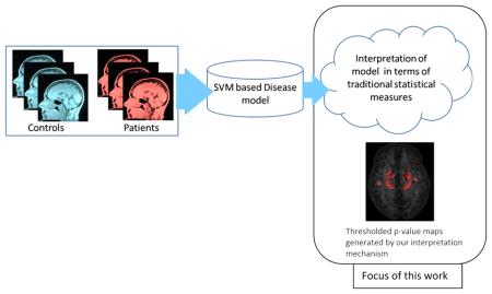
Understanding spatial imaging patterns associated with normal or pathologic structure and function of the brain is a major focus in neuroimaging. The simplest and the most prolific approaches to address this problem stem from early work in mass univariate data analysis. For instance, voxel based morphometry Ashburner and Friston (2000) Friston et al. (1993) Chung (2012) for population wide neuroimaging analysis still remains one of the most informative and useful tools in the neuroimaging community. However, relatively recent developments have lead to the emergence of a new class of methods for analyzing neuroimaging data. Machine learning based methods Davatzikos (2004) Cuingnet et al. (2011) De Martino et al. (2008) Fan et al. (2007) Gaonkar and Davatzikos (2012) Xu et al. (2009) Van De Ville et al. (2007) Van De Ville et al. (2004) Mingoia et al. (2012) can offer diagnostics based on neuroimaging data. Such diagnostic scores are especially relevant in the study of neurological diseases. An important characteristic of these machine learning methods is that they utilize information from the entire image in order to deliver the diagnosis. This is distinctly different from using information related to one or another region gleaned from a mass univariate analysis. Thus, machine learning based methods are especially well suited for imaging based diagnosis of neurological diseases in which the etiological mechanism might involve patterns of deficits in several brain regions acting together as opposed to focal lesion like pathologies. Thus, it is critical to identify the specific brain regions that the diagnostic scores produced by these methods are based on. This is the general focus of the current work. Specifically the current work focuses on interpreting neuroimaging based disease models generated by support vector machines (SVMs) Vapnik (1995) Burges (1998). SVMs have been widely used in the neuroimaging community to generate diagnostic scores on the basis of brain images Mouro-Miranda et al. (2005) Wang et al. (2007) Cuingnet et al. (2011) Craddock et al. (2009) Fan et al. (2007) Batmanghelich et al. (2012) Vemuri et al. (2008) Davatzikos et al. (2011).

While SVMs use multivariate imaging information to make decisions, tracing the pattern of brain regions most relevant to the SVM decision is a non trivial pursuit. A mechanism for tracing these patterns using the widely understood statistical p-values is the primary topic of this work. It should be noted that in the low dimensional high sample size setting confidence intervals associated with the Hotelling T²- statistic Morrison (1967) provide such a mechanism. However, the Hotelling T²- statistic is not estimable in the high dimension low sample size setting encountered in medical imaging. Further, while machine learning literature does provide mechanisms for ranking features using algorithms based on various criteria and constraints, these do not always provide inference in terms of the generally well understood and widely used statistical p-values. The clinical community prefers statistical p-values partly due to clinical training and partly because p-values provide a mathematically rigorous way of determining whether an observed pattern could be obtained by chance from the null distribution.

1.2. Background

Now, we attempt to place the current work in the context of existing literature. Before we delve into related work it is important to bear in mind that the primary focus of this work is to understand what regions of the brain are utilized by a support vector machine model to deliver diagnostic scores (such as the scores described in Klöoppel et al. (2008) or Fan et al. (2007)). Thus, the question we wish to address is: Which regions does an SVM model use to make the diagnosis? This is slightly different from the question that is the subject of more traditional multi/univariate analyses which is : Which specific regions differ between two groups that are apriori known to be distinct? Nevertheless, we put our work in the context of both paradigms. We will explain the differences between these paradigms and their relation to the presented work in the following paragraphs.

Pioneering work that applied multivariate analysis to functional time series data was presented in Friston et al. (1995) Friston et al. (1993). Eigen-analysis for functional data analysis was presented in Friston (1997). Early work in McIntosh et al. (1996) described the extraction of multivariate spatial patterns using partial least squares regression. Related work regarding model selection in multivariate analysis was presented in Kherif et al. (2002). While a substantial portion of early work still focussed on voxel specific multivariate effects, it paved the way for later development of the field of multivariate analysis.

Independent components analysis (ICA) was one of the earliest of multivariate analysis methods. It remains one of the most prolific methods used for fMRI data analysis Xu et al. (2009) McKeown and Sejnowski (1998) Smith et al. (2004) Svenséen et al. (2002) Stone et al. (2002) Perlbarg et al. (2007). SVM Wang et al. (2007) Cuingnet et al. (2011) Craddock et al. (2009) Fan et al. (2007) Batmanghelich et al. (2012) Vemuri et al. (2008) Davatzikos et al. (2011) Mouro-Miranda et al. (2005) based tools for imaging based diagnoses came a little later and addressed a paradigm completely different from that of ICA. We build upon this work in SVM based neuroimaging analyses. Our focus in this paper is rather narrow. Specifically we focus on developing a statistical inference framework for interpreting diagnostic models provided by the SVM.

While the p-values produced by our inference framework may be applied to improve the interpretability of neuroimaging based SVM classifier it should not be confused for multivariate statistical testing frameworks like MANOVA Casella and Berger (2002) Srivastava and Du (2008) Fujikoshi et al. (2004) (or its equivalents). It should also not be confused with assessing the overall significance of the accuracy of classification. Work by Golland and Fischl (2003) Ojala and Garriga (2010) Hsing et al. (2003) Pesarin and Wiley (2001) is more relevant to addressing these problems. Also, in the strictest sense, our framework should be considered complementary to local univariate/multivariate analyses that are commonly used for identifying neuroimaging based differences between populations.

The primary differences between our approach and approaches like voxel based morphometry (VBM)/SVM searchlights Xiao et al. (2008) Rao et al. (2011) Etzel et al. (2013)) are 1) that our approach focusses on interpreting an SVM model and 2) that our approach is based on a global perspective that considers an image as a single high dimensional point. Consequently, the p-values generated from our method may not suffer from some of the limitations of searchlights described in Etzel et al. (2013) and the limitations of univariate methods described in Davatzikos (2004). This is because some of the limitations described by Etzel et al. (2013) and Davatzikos (2004) are primarily due to a relatively local scope of the respective analyses.

Specifically, SVM searchlights use cross validation to derive a p-value for the separability of the local multivariate patterns. It is possible that an SVM classifier training to identify disease using image data, due to its global scope, uses a combination of regions that are invisible to the relatively local searchlight/VBM analyses. However, it is equally likely that an SVM classifier trained as such does not utilize a large portion of regions that actually differ between patients and controls to make its diagnostic decision. It is always important to bear in mind that while machine learning approaches such as the SVM perform multivariate analysis, they do so with the express aim of estimating/training a function that can predict a variable of interest (e.g. patients vs. controls) from the pattern over a set of variables (voxel intensities). Thus, the patterns of p-values identified by the use of the searchlight may be distinct from that identified using the work presented here because the two approaches ultimately ask different questions. The searchlight asks whether a specific region differs between two groups. The approach presented here attempts to address the question: how important a specific region is to an SVM model trained to distinguish between two groups.

In a certain sense the the work presented here is the SVM counterpart of recent work by Bühlmann and Van De Geer (2011) in addressing the statistical inference problem for L1-regularized high dimensional regression methods (related to the LASSO). These methods can be modified to yield p-values as well. However, LASSO and L1-regression based methods are designed to eliminate redundant features Zou and Hastie (2005) to a much greater extent than L2-regularized methods such as SVMs. They are also quite sensitive to regularization Gaonkar and Davatzikos (2013). Thus, in the extremely high dimensional setting in neuroimaging these may not be ideal unless the dimensionality is reduced to something smaller than the sample size available. It should be noted that in the low dimension high sample size setting these methods can be very effective. Good examples of using the LASSO in imaging are fMRI analysis presented in Bunea et al. (2011) and shape analysis presented in Kim et al. (2012); Chung (2012).

Further, this section would perhaps be incomplete without mentioning the work of Cuingnet et al. (2011) and Rasmussen et al. (2011) both of which influenced the drafting of this document. Specifically, Cuingnet et al. (2011) introduced us to the concept of SVM based permutation testing. The work by Rasmussen et al. (2011) generalizes the concept of SVM weight based visualization to kernel based non-linear classification frameworks. While there exist certain disadvantages to using SVM weights directly (see Cuingnet et al. (2011)), the work by Rasmussen et al. (2011) provides a roadmap for future development of this method.

It is also important to note that work presented here draws heavily upon our recent work from Gaonkar and Davatzikos (2013). Thus, we have summarized certain sections of our previous work here and reproduced certain derivations in the appendix. In Gaonkar and Davatzikos (2013) we showed that the null distribution of SVM weight vectors estimated via permutation tests is asymptotically normal in high dimension low sample size settings found in neuroimaging. In Gaonkar and Davatzikos (2013) we followed previously published neuroimaging literature which used the components of SVM weight vector as permutation statistics. However, we later realized that using SVM weight vector components directly ignored the most important aspect of SVM theory, namely the margin. Classification with a wider margin is inherently better than classification with a narrower one (see figure 1). This is the basis of SVM theory (Vapnik, 1995). Using w alone, risks accepting the null hypothesis even when the margin associated with SVM classification is very high leading to very conservative inference. Thus, permutation testing must be done with a statistic that is margin aware. This paper focuses on the development of an inference framework using such a statistic.

Figure 1.

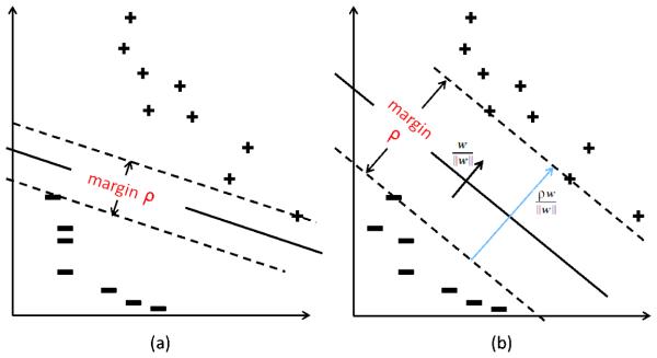
(a) Classification hyperplane with small margin (b) Classification hyperplane with larger margin preferred by SVM optimization. Also shown is the vector $\frac{\rho \mathbf{w}}{\parallel w\parallel }$ which encodes margin information and is proportional the statistic used in this paper.

Thus, we are proposing a margin aware analytic inference framework for interpreting SVM models in neuroimaging. This is motivated by 1) a need for a clinically understandable, p-value based, way to interpret SVM models that accounts for SVM margins explicitly and 2) the need for a fast and efficient tool for multivariate morphometric analysis in the face of ever increasing dimensionality of medical imaging (and other) data.

In the following sections we build upon the work in Gaonkar and Davatzikos (2013) and Cuingnet et al. (2011) to 1) present and explore a margin aware statistic that can be used to interpret SVM models using permutation tests 2) develop analytic null distributions that can be coupled with the proposed statistic for inference 3) present results for validating the proposed analysis and its approximation using suimulated and actual neuroimaging data. We collect our thoughts on contributions,limitations and future work associated with the method in the discussions section before concluding the manuscript.

2. Materials and Methods

2.1. Permutation testing with SVMs

In this subsection we specifically stress upon certain aspects of previous work that are critical to understanding this paper. We state the main results necessary for developing the margin aware statistic. We have reproduced sections of the original work Gaonkar and Davatzikos (2013) in the appendix that delve into the detail of the derivations that drive these results. In what follows we briefly review SVM theory, permutation testing on SVM theory and the main result of Gaonkar and Davatzikos (2013).

Given preprocessed brain images corresponding to two known labels (eg. normal vs. pathologic, activated vs. resting) , the SVM solves a convex optimisation problem under linear constraints that finds the hyperplane that separates data pertaining to the different labels with maximum margin. This hyperplane minimizes ‘structural risk’ (Vapnik, 1995) which is a specific measure of label prediction accuracy that generalizes well in high dimensional space. Given an image of a patient whose status is unknown, the SVM can then use the previously obtained hyperplane (also called learnt model) to predict the labels. The process of learning this model from data in which the state labels are known is called training. The process of predicting state labels for previously unseen imaging data is called testing.

In SVM theory the data are represented by feature vectors with the i^th image being represented by the vector x_i ∈ ℝ^d. We require that all images contain the same number d of informative voxels. Pathological (or functional) states are typically denoted by labels y_i ∈ {+1, −1}. For instance, these labels might indicate the presence/absence of stimulus or disease. The SVM model is parameterized by w ∈ ℝ^d which can be visualized as a d- dimensional hyperplane (see figure 1). Explicitly the problem solved can be written as:

$$\begin{array}{cc}\hfill & \{{\mathbf{w}}^{\ast },b^{\ast }\}=argmin{}_{\mathbf{w},b}\frac{1}{2}\parallel \mathbf{w}{\parallel }^2\hfill \\ \hfill & subj.to.y_i({\mathbf{w}}^T{\mathbf{x}}_i+b)\ge 1{\forall }_i=1,\dots ,m\hfill \end{array}$$ (1)

Note that m is the number of subjects in the training data. Also note that we do not include the SVM slack term. This is based on the reasoning that the inclusion of the slack variables in the SVM formulation is primarily to allow for a feasible solution in the absence of perfect separability of the data with respect to the labels (Vapnik, 1995). Thus, in high dimension low sample size data, where perfect separability is guaranteed the solutions of the hard and soft margin SVMs should essentially be the same, except for very small values of C.

The SVM algorithm described above associates a weight vector coefficient $w_j^{\ast }$ with every dimension of the input space. In imaging this corresponds to a specific voxel. While the weight map itself has been used for interpreting SVM models Rasmussen et al. (2011) Guyon et al. (2002), it has been noted that using SVM weights can assign relatively low weights to significant features and relatively larger weights to irrelevant features Hardin et al. (2004) Cuingnet et al. (2011) Gaonkar and Davatzikos (2013). We have also documented this behavior in figure 4 and the associated experiment. A second shortcoming of a purely weight based interpretation is the lack of a statistical p-value based inference. As explained earlier, a p-value based inference machinery can be of a distinct advantage for communicating results to non specialist collaborators in the clinical community. Some of these limitations of can be overcome by using SVM weights as statistics for permutation testing. Permutation testing involves the generation of a large number of shuffled instances of data labels by random permutations Pesarin and Wiley (2001). Each shuffled instance is used to train one SVM. For each instance of shuffled labels, this generates one hyperplane parameterized by the corresponding vector w. Then for any component of w, we have one value corresponding to a specific shuffling of the labels. Collecting the values corresponding to any one component of w allows us to construct a null distribution for that component of w. Recall that each component of ‘ w’ corresponds to a voxel location in the original image space. Thus, permutation testing leads to a null distribution associated with every voxel in the image space.

Figure 4.

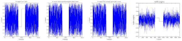
Inference on multivariate toy data p-values generated using standard t-tests (left) Inference using experimental permutation tests (middle-left) Inference using analytic permutation tests (middle-right) Inference using SVM weights (right)

One can use the Lyapunov central limit theorem to show that these null distributions are normal and have a mean and variance can be predicted from the data. This was the primary contribution of our previous work Gaonkar and Davatzikos (2013). We have reproduced a short version of the derivation of this normality in the appendix of this manuscript. Essentially, If X ∈ ℝ^m×d is a matrix with d >> m and y ∈ ℝ^m is a set of randomly permuted labels corresponding to images in X, SVM solutions associated with a majority of the permutations can be approximated by solving a much simpler problem:

$$\begin{array}{cc}\hfill & mi{n}_{\mathbf{w},b}\parallel \mathbf{w}{\parallel }^2\hfill \\ \hfill & subj.to.\mathbf{X}\mathbf{w}+\mathbf{J}j=y\hfill \end{array}$$ (2)

The solution to this problem may be written as:

$$\mathbf{w}\approx \mathbf{Cy}$$ (3)

where:

$$\mathbf{C}={\mathbf{X}}^{\mathbf{T}}[{\left({\mathbf{XX}}^{\mathbf{T}}\right)}^{-1}+{\left({\mathbf{XX}}^{\mathbf{T}}\right)}^{-1}\mathbf{J}{(-{\mathbf{J}}^{\mathbf{T}}{\left({\mathbf{XX}}^{\mathbf{T}}\right)}^{-1}\mathbf{J})}^{-1}{\mathbf{J}}^{\mathbf{T}}{\left({\mathbf{XX}}^{\mathbf{T}}\right)}^{-1}]$$ (3)

with J ∈ ℝ^m being a vector with each component equal to 1.

Since permutation testing involves random relabelling of the data, the majority ofpermutations use labels which do not coincide with y. In the absence of labels that correspond to any meaningful phenomenon in the data, we expect the generalization error of the corresponding SVM model to be high. Given the high dimensionality we expect gross over fitting to achieve the minimum in equation 1. Since learning is ultimately based on data compression Kearns and Vazirani (1994) we may conjecture, for random permutations no compression will be achieved by the SVM. The SVM model might just store all the samples and the respective labels. In the specific context of SVMs this may lead to most (if not all) samples becoming support vectors. Conjecture apart, we actually observed this phenomenon in experiments performed with structural and functional neuroimaging datasets as documented in Gaonkar and Davatzikos (2013). This phenomenon ultimately lead us to equation (3)

Since the equation (3) ultimately expresses SVM weights as linear combinations of the labels one can establish the asymptotic gaussianity of the distribution of SVM weights (produced by the permutation procedure) using the Lyapunov central limit theorem (see appendix). Indeed, the null distribution of w_j (the j^th component of w) is given by:

$$\frac{w_j-{\mu }_j}{{\sigma }_j}\stackrel{n}{\to }\mathcal{N}(0,1)$$

as m → ∞ with

$${\mu }_j=(2p-1)\sum _{i=1}^m{C}_{ij}{\sigma }_j^2=(4p-4p^2)\sum _{i=1}^m{C}_{ij}^2$$ (5)

with i ∈ {1, ….,m} indexing the samples, j ∈ {1, …,d} indexing voxels and p being the fraction of labels that are +1. To obtain p-values for a specific voxel we need to compare the $w_j^{\ast }$ computed using the original labels to the distribution given by (5). However, as stated earlier, the main theme of this work is that these p-values do not account for margin information. Hence, we use an alternate statistic which we describe next.

2.2. The margin aware statistic

In this section we describe the intuition behind a ‘margin aware’ statistic for SVM based permutation testing and contrast it to the statistics we used in our previous work. We also present a strategy for approximating permutation based null distributions associated with this statistic.

Suppose ρ is the margin associated with an SVM classifier trained on a specific permutation of the labels. Then we want to compute the null distribution of

$$s_j=\frac{\rho }{2}\frac{w_j}{\parallel \mathbf{w}\parallel }$$ (6)

The statistic s_j represents the components of the vector $\frac{\rho \mathbf{w}}{\parallel \mathbf{w}{\parallel }^2}$ that is perpendicular to the separating hyperplane and has magnitude proportional to the margin associated with the classifier. The index j counts over voxels.

The intuition behind this definition is presented in figure 1.

SVM theory dictates that it is not only the direction of the hyperplane but also the margin that it achieves which makes it superior to competing solutions. This is in fact the heart of the SVM formulation and also the reason for its success in high dimensional classification. It is known that increased margin generally corresponds to a higher classification accuracy for SVMs. The quantitative embodiment of this assertion is the radius margin bound on the generalization error of the SVM Burges (1998)(Vapnik, 1995). Yet, the statistics used in a large proportion of previous work, Gaonkar and Davatzikos (2013) Mouro-Miranda et al. (2005) Wang et al. (2007) Rasmussen et al. (2012) Rasmussen et al. (2011) including our own, completely ignores the margin. Using s_j instead of w_j for permutation testing incorporates the higher confidence associated with a higher margin directly into the statistical p-values generated by the permutation procedure and this in turn yields better interpretation as evidenced by experiments here and elsewhere Cuingnet et al. (2011). The rest of this section focusses on developing an analytic expression for estimating the null distribution of s_j. In order to approximate these distributions we first note that the SVM margin can be written in terms of the weight vector as:

$$\rho =\frac{2}{\parallel \mathbf{w}\parallel }$$

Thus the statistic s_j can be written as:

$$s_j=\frac{w_j}{\left({\mathbf{w}}^T\mathbf{w}\right)}$$ (8)

In order to approximate the null distributions of s_j we use (5) and note that for C given by (4) we have:

$$\mathbf{CJ}=0$$ (9)

Thus:

$$\sum _{i=1}^m{C}_{ij}=0\Rightarrow {\mu }_j=0\Rightarrow E\left(w_j\right)=0$$ (10)

We then proceed using classical (see (Casella and Berger, 2002), example 5.5.27 on page 245) Taylor asymptotic approximations to estimate the mean and the variance of s_j:

$$E\left(s_j\right)=E\left(\frac{w_j}{{\mathbf{w}}^T\mathbf{w}}\right)\approx \frac{E\left(w_j\right)}{E\left({\mathbf{w}}^T\mathbf{w}\right)}=0$$ (11)

And similarly we can approximate the variance as:

$$\begin{array}{cc}\hfill var\left(s_j\right)& \approx \frac{var\left(w_j\right)}{E{\left({\mathbf{w}}^{\mathbf{T}}\mathbf{w}\right)}^2}+\frac{E{\left(w_j\right)}^2}{E{\left({\mathbf{w}}^{\mathbf{T}}\mathbf{w}\right)}^4}var\left({\mathbf{w}}^T\mathbf{w}\right)\hfill \\ \hfill & -2\frac{E\left(w_j\right)}{E{\left({\mathbf{w}}^{\mathbf{T}}\mathbf{w}\right)}^4}cov(w_j,{\mathbf{w}}^{\mathbf{T}}\mathbf{w})\hfill \\ \hfill & =\frac{var\left(w_j\right)}{E{\left({\mathbf{w}}^{\mathbf{T}}\mathbf{w}\right)}^2}\hfill \end{array}$$ (12)

We estimate E(w^Tw) using the theory of quadratic forms (Searle, 2012):

$$E\left({\mathbf{w}}^T\mathbf{w}\right)=tr\left({\Sigma }_w\right)+{\mu }^{\mathit{T}}\mu \sum _{k=1}^d({{\sigma }_k}^2+{\mu }_k^2)=\sum _{k=1}^d{{\sigma }_k}^2$$ (13)

Thus, we can write (12) as:

$$var\left(\frac{w_j}{{\mathbf{w}}^{\mathbf{T}}\mathbf{w}}\right)\approx \frac{var\left(w_j\right)}{E{\left({\mathbf{w}}^{\mathbf{T}}\mathbf{w}\right)}^2}=\frac{{\sigma }_j^2}{{\left[\sum _{k=1}^d{\sigma }_k^2\right]}^2}$$ (14)

Further, since s_j may be written as a continuous and smooth function of the components of w which are themselves normally distibuted with a positive definite co-variance matrix, we have that s_j is approximately normally distributed by the multivariate delta method (Casella and Berger, 2002):

$${\left(\frac{{\sigma }_j}{\left[\sum _{k=1}^d{\sigma }_k^2\right]}\right)}^{-1}{s}_j\stackrel{d}{\to }\mathcal{N}(0,1)$$ (15)

2.3. About the Alzheimers disease neuroimaging initiative (ADNI)

Data used used in the preparation of this article were obtained from the ADNI database (adni.loni.ucla.edu). The ADNI was launched in 2003 by the National Institute on Aging, the National Institute of Biomedical Imaging and Bioengineering, the Food and Drug Administration, and private pharmaceutical companies and non-profit organizations as a $ 60 million, 5-year publicprivate partnership. The primary goal of ADNI has been to test whether serial magnetic resonance imaging, positron emission tomography, other biological markers, and clinical and neuropsy-chological assessment can be combined to measure the progression of MCI and early AD. Determination of sensitive and specific markers of very early AD progression is intended to aid researchers and clinicians to develop new treatments and monitor their effectiveness, as well as lessen the time and cost of clinical trials.

The principal investigator of this initiative is Michael W. Weiner, MD, VA Medical Center and University of California San Francisco. ADNI is the result of efforts of many co-investigators from a broad range of academic institutions and private corporations, and subjects have been recruited from over 50 sites across the USA and Canada. The initial goal of ADNI was to recruit 800 adults, ages 5590years, to participate in the research, approximately 200 cognitively normal older individuals to be followed up for 3years, 400 people with MCI to be followed up for 3years, and 200 people with early AD to be followed up for 2years. For up-to-date information, see www.adni-info.org.

The data collection and sharing for this project was funded by the Alzheimer’s Disease Neuroimaging Initiative (ADNI) (National Institutes of Health Grant U01 AG024904). ADNI is funded by the National Institute on Aging, the National Institute of Biomedical Imaging and Bioengineering, and through generous contributions from the following: Abbott, AstraZeneca AB, Bayer Schering Pharma AG, Bristol-Myers Squibb, Eisai Global Clinical Development, Elan Corporation, Genentech, GE Healthcare, GlaxoSmithKline, Innogenetics, Johnson and Johnson, Eli Lilly and Co., Medpace, Inc., Merck and Co., Inc., Novartis AG, Pfizer Inc, F. Hoffman-La Roche, Schering-Plough, Synarc, Inc., as well as non-profit partners the Alzheimer’s Association and Alzheimer’s Drug Discovery Foundation, with participation from the U.S. Food and Drug Administration. Private sector contributions to ADNI are facilitated by the Foundation for the National Institutes of Health (www.fnih.org). The grantee organization is the Northern California Institute for Research and Education, and the study is coordinated by the Alzheimer’s Disease Cooperative Study at the University of California, San Diego. ADNI data are disseminated by the Laboratory for Neuro Imaging at the University of California, Los Angeles. This research was also supported by NIH grants P30 AG010129, K01 AG030514, and the Dana Foundation.

3. Experiments and Results

3.1. Simulated data

In this section we present inference on simulated datasets using the proposed framework. The primary aim of this section is to demonstrate the validity of the proposed machinery. We show that the proposed statistic can indeed identify features/regions we would expect the SVM model to utilize for making a diagnosis. The other objective is to emphasize the non incremental value of this work by highlighting the difference between the margin based statistic proposed here and permutation testing based on the SVM weights themselves (Gaonkar and Davatzikos, 2013)(Gaonkar and Davatzikos, 2012).

We simulate high dimension low sample size data that contain univariate and multivariate effects of interest which differentiate two subsets of the data. When single features (voxels in neuroimaging; genes and measures of their expression in genomics) can be used to detect differences between two groups, we say that a univariate effect is present at that feature. When one feature has to be used in conjunction with another (or many other) features to distinguish between two groups we say that multivariate effects are present. We simulate data with both univariate and multivariate effects and show that our framework can be used to identify these effects. We also contrast our method with the widely used univariate analyses.

3.1.1. Detection of simulated univariate effect

The aim of simulation was to show that the proposed method can detect regions that differ between groups in a univariate sense. The data simulation involves 1) generation of random noise data X ∈ ℝ^100×2000 by sampling a standard uniform distribution 2) random assignment of labels +1 and −1 to the 100 samples 3) subtracting a fixed value of 0.3 from 350 features in all samples labeled +1. The results are presented in figure 2. The intention here was to simulate an effect which could easily be detected using a t-test. This can be seen from the low p-values assigned by the t-tests to the subtraction region in figure 2. The SVM based permutation test using the margin aware statistic can find this region as well. The analytic approximation to the margin based statistic is equally effective in identifying the required region. Thus, the performance of our proposed statistic is comparable to the t-test when pure univariate effects can differentiate between data.

Figure 2.

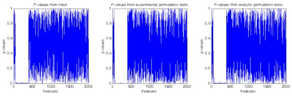
Inference for data where univariate effects may be used to distinguish labels (left) with p-values calculated by t-tests (middle) p-values calculated by permutation testing using the margin aware statistic and (right) p-values calculated by the analytical approximation to permutation testing using the margin aware statistic

3.1.2. Detection of simulated multivariate effect

We consider multivariate effects be present when only a combination of two or more features can separate positively and negatively labelled samples. The simplest illustration of a simulated multivariate effect is shown in figure 3 where the green circles and blue crosses indicate distinct labels. The x and the y co-ordinates of each point represent values of features. Note that either x or y, used alone cannot differentiate blue from green. However, when used together one can easily draw a line that separates blue from green on the plot. This is why multivariate predictive analysis is considered superior to univariate analysis. The simulation scheme used to obtain data separable using a multivariate effect is illustrated in figure 3.

Figure 3.

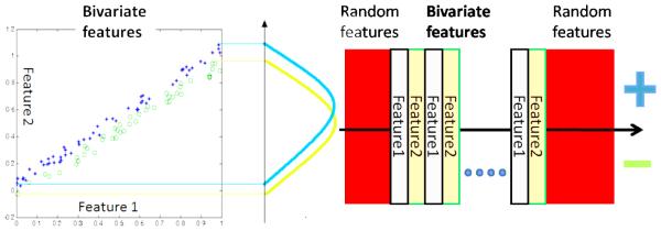
(Left) Features which can be used in a combined way but cannot be used individually to separate categories (Right) Illustration depicting simulation procedure for generation of multivariate toy data

The procedure consists of generation of bivariate features and corresponding labels (such as those illustrated by figure 3) followed by addition of random noise features. To generate the bivariate features we 1) sample 100 points (z_i) from a standard uniform distribution 2) sample points u_i from the standard normal distribution. 3) choose a factor f < 0.1 and generate point pairs (z_i, z_i + fu_i). 4) generate labels using the criterion label = sign(fu_i). A plot of a specific set of these pairs is shown in figure 3. In order to simulate such an effect in high dimensions we horizontally stack 200 of these point-pairs as indicated by the gray-orange rectangles in figure 3 leading to a total of 400 signal features. We also add 1600 noise features (indicated by red rectangles). These are generated by sampling the standard uniform distribution. Thus we have 100 samples and 2000 features. This simulates the high dimension low sample size setting. For inference purposes we run t-tests, actual permutation tests using the margin aware statistic and the analytic permutation tests proposed. The results are presented in figure 4. We also show SVM weights corresponding to the simulated features in figure 4 for comparison purposes. The figure shows that SVM weights or t-tests alone may not be sufficient to identify regions that the SVM model uses for classification. Using permutation testing to model the variance of the weights provides a certain edge over using the weights directly or over univariate testing in this sense.

3.2. Why permutation testing with margin based statistics is better than permutation testing with SVM weights

In our previous work we proposed the use of permutation tests on SVM weights for interpreting SVM models (Gaonkar and Davatzikos, 2013). We showed in (Gaonkar and Davatzikos, 2013) that this approach compares favorably with the use of standard univariate analysis as well as with using the weight vectors themselves. The method also had lower false positive detection rates as compared to univariate analysis. However, with additional experimentation we found the method to be lacking in one key aspect. The method presented in (Gaonkar and Davatzikos, 2013) is highly sensitive to the size of the abnormality (see figure 5). This is because SVM weights associated with each voxel/feature get smaller if the number of voxels/features driving the group difference increase. This raises the p-values associated with these features and reduces the sensitivity of the associated p-value map. In this sense using ‘w’ alone seems to work more like the LASSO or the elastic net. We show here through simulated experiments that the margin based statistic alleviates this shortcoming of the original method.

Figure 5.

(Left column) p-values generated using t-tests with red circles indicating the location of the ground truth simulated effects (Middle column) p-values generated using SVM weights alone as described in (Gaonkar and Davatzikos, 2013). Note that as the size of the simulated abnormality is increased the p-values increase to as high as p=0.8. Orange circles indicate the approximate location of ground truth (Right column) p-values generated using the margin based statistic. Green circles indicate approximate location of ground truth.

3.2.1. Effect of simulated abnormality size on the analysis

In order to demonstrate the increased sensitivity of the weight based statistic to the size of the abnormality we create 3 separate datasets. Each of these datasets have their own simulated abnormality. The procedure used to create the data includes 1)generation of a random noise matrix of size ℝ^100×1000 2) Randomly labeling 50 of these samples as +1 and the other 50 as −1. 3) Subtracting 0.3 from a pre-chosen subset of the 1000 features. Depending of the effect desired we chose either 50, 150 or 250 features from which the subtraction was made. For each of these datasets we show a plot of p-values generated using a) univariate testing b) the analytic approximation to the SVM weight vectors presented in (Gaonkar and Davatzikos, 2013) c) The analytic testing framework proposed in this paper. These results are shown in the figure 5. From figure 5, we see that 1) using permutation tests based on SVM weights can detect small abnormalities 2) as the dimensionality increases, p-values based SVM weights can get as high as 0.8-0.9 which makes the abnormality undetectable at the standard threshold (α = 0.05) 3) The margin based p-value is relatively robust in this respect. In the following subsection we present similar results in neuroimaging data with simulated abnormalities.

3.2.2. Neuroimaging data with simulated abnormalities of different sizes

All the previously presented simulations use simulated effects as well as simulated noise. In order to bring the simulations closer to actual neuroimaging data we present a few experiments in this subsection using actual neuroimaging data. For this experiment we used grey matter tissue density (RAVENS (Davatzikos et al., 2001)) maps generated using ADNI data that was provided to us by authors of (Davatzikos et al., 2011). These maps are generated using an established pipeline which will be described in the section, ‘Experiments on ADNI data: qualitative analysis’. The use of these maps as opposed to the raw images provides feature correspondence across the sample. Establishing such correspondence is a non-trivial image processing task that the authors of (Davatzikos et al., 2011) have addressed.

We chose 152 grey matter RAVENS maps , from selected normal controls and introduced simulated an abnormality in exactly 76 of them. The region in which the abnormality was to be introduced was painted in using ITK-SNAP (Yushkevich et al., 2006). The abnormality is simulated by reducing the map intensity by 30%.

We used both SVM weight based permutation tests (Gaonkar and Davatzikos, 2013) and the margin based statistic described here to analyze the data. We also performed the above simulation with both, a small and a large simulated abnormality. The results are shown in figure 6. In general the following conclusions may be drawn from figure 6: First even in the presence of the noise profile associated with actual neuroimaging data, the proposed method of inference performs well. Second, this experiment re-iterates the finding that inference based on permutation tests using SVM weights is highly sensitive to the size of the simulated abnormality. The margin based statistic does not seem to suffer from this problem.

Figure 6.

Detecting focal and non-focal simulated effects in neuroimaging data. First two columns from the left show detection using proposed statistic. Third column shows regions detected using permutations based on SVM weights only. The last column shows ground truth

3.3. Experiments with ADNI data: Qualitative analysis

We describe experiments with regional tissue density (RAVENS (Davatzikos et al., 2001)) maps generated using Alzheimer’s disease (ADNI) data that was provided to us by authors of (Davatzikos et al., 2011).

This data was generated from raw T1-images by processing them through a series of pre-processing steps. The preprocessing protocols included a) skull removal using the BET algorithm (Smith, 2002) b) n3 bias correction using N3(Sled et al., 1998) c) segmentation using adaptive k-means (Pham and Prince, 1999) d) registration to a common template and generation of RAVENS maps using the (Davatzikos et al., 2001) protocol. The data provided were in the form of grey matter , white matter and ventricular tissue density (Davatzikos et al., 2001) maps. We chose 100 controls and 100 patients from the provided dataset to run these experiments. For each subject all 3 RAVENS maps were concatenated into a single feature vector. Thus we obtained one feature vector per subject. One thousand SVMs were trained using random permutations of the labelings (controls and patients) to obtain the null distributions of the proposed statistics for these subject specific feature vectors. These null distributions were used to compute experimental p-values. The analytical p-values were obtained using the distributions described by our framework (15).

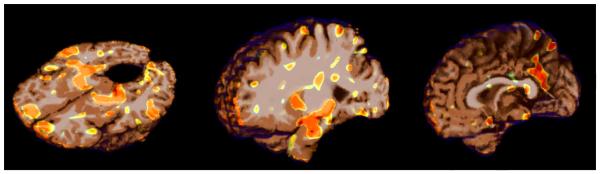
Figure 7 shows volumetric renderings of the negative logarithm of p-values corresponding to the grey matter tissue density maps overlaid on a brain volume. We include renderings for both analytically and experimentally obtained p-values overlaid on the T1-brain image. It can be seen from these images that the experimental and analytic p-value maps are at least visually indistinguishable. Based on our simulated experiments we interpret regions with lower p-values (higher -log(p-values)) to be more important to the classification function. Regions identified by thresholding the p-map using the Benjamini-Yekutieli procedure at a q-value((Benjamini and Yekutieli, 2001)) of 0.1 are shown in figure 8. Upon thresholding the p-map using the Bonferroni procedure at α = 0.05 only the hippocampi are highlighted (See figure 9). Despite the usefulness of the two corrected p-value maps we surmise that the the negative log p-value maps of figure 7 provide for a better depiction of the relative importance of different brain regions in relation to the SVM model. While figures 7,8 and 9 provide a visual description of the SVM p-value maps on ADNI data, for the sake of completeness we have included a more quantitative picture of the approximation in the scatter plot presented in figure 11. We also present briefly a quantitative analysis of the error of approximation (w.r.t. actual permutation testing) in section 6.

Figure 7.

Visual comparison of experimentally (left) vs analytically (right) generated -log(p-value) maps on ADNI data

Figure 8.

Regions detected after applying multiple comparisons corrections using the Benjamini-Yekutieli procedure at q ≤ 0.1

Figure 9.

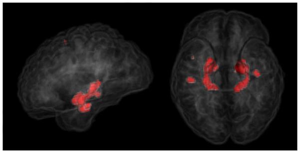
Regions detected after applying multiple comparisons corrections using the Bonferroni correction at α = 0.05

Figure 11.

Scatter plots comparing actual permutation testing with analytical approximation

3.4. Experiments with ADNI data: Comparison with local univariate analysis

As described in the introduction the primary focus of this work is to understand what regions of the brain are utilized by a support vector machine model to deliver diagnostic scores from imaging data. Thus, we are addressing the global multivariate paradigm and asking the question: What network of interacting regions does this SVM model use to make the diagnosis? This is slightly different from the local paradigm that is typically a subject of more traditional local univariate analyses which is : Which specific regions differ between two groups which are apriori known to be distinct?

The SVM models are thought to utilize global structural or functional imaging patterns to differentiate between groups. Thus, SVM based analyses may be suitable to identify a network of regions that acts synergistically to manifest a group difference. In contrast local univariate analyses may be more suitable to identify how a specific region differs between two groups. Thus, there is an inherent complementarity between these two types of analyses. We demonstrate this complementarity by comparing the result of a univariate analyses to that of the proposed multivariate analyses on ADNI data in figure 10.

Figure 10.

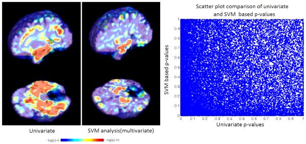
Complementary nature of SVM based analysis and univariate analysis (left) scatter plot of p-values obtained from univariate and multivariate analyses (right)

The univariate p-value map shown in figure 10 is generated by performing two sample t-tests between the grey matter tissue density values at individual voxels. The analytical approximation to permutation testing is used to generate the SVM based p-value map. A scatter plot comparing p-values obtained from the two analyses is also included in figure 10. The scatter plot shows that the two p-value maps are distinct. Some regions such as the hippocampi are significant according to both p-value maps. However, some other regions such as the orbito-frontal lobes are better highlighted in the SVM based map. Other regions in the temporal lobe are seem more clearly in univariate analysis. These results are not necessarily novel, but are simply presented here as a confirmation of the the view that local univariate analyses and global SVM based multivariate analyses offer complementary information for population based statistical analysis.

Further, it is also important to remember that the multivariate analysis presented here is focussed on interpreting the SVM model. Thus, we might say that the SVM uses a global pattern involving the hippocampus in combination with the highlighted regions of the orbito-frontal cortex to make its predictions. This, the SVM does despite the fact that the univariate voxelwise differences between patients and controls in this region are not as strong as some other regions in the temporal lobe.

Thus, we may interpret, to successfully achieve better separation between controls and patients in a multivariate sense, the SVM model relied not only on the hippocampus and the temporal lobe but also on the orbito-frontal regions. Further, the SVM leave one out cross-validation accuracy of 87% gives us an idea of the predictive power of the highlighted multivariate pattern. As such there is no comparable measure to cross-validation accuracy in univariate analysis.

Further, it is important to remember that interpretations based on the SVM p-value maps (just as is the case VBM or with looking at SVM weights) can only provide qualitative guidelines as to what fundamentally drives classification with SVMs and what ultimately drives disease. The pathophysiology that drives a specific disease is likely to be far more complicated than what can be gleaned using any of these methods alone.

3.5. Quantitative analysis

We present scatter plots between experimental and analytical p-values in figure 11. The approximation accuracy seems to be higher at the low and high p-value ranges. These plots are based off the data used for generating figures 2,4 and the ADNI data.

The convergence between the analytic p-values and the experimental ones as measured by the average per voxel error is rapid. From figure 12 we can see that the average per voxel error in the p-values does not change substantially whether one uses 500 permutations or 1000 permutations. It does change substantially if one uses 100 permutations rather than 50. This was one of the factors behind choice of one thousand permutations for our experiments.

Figure 12.

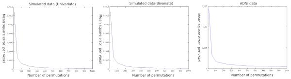
Convergence of the analytical approximation to experimental permutation tests

To investigate the behaviour of the approximation at ultra low p-values, we plot the negative logarithm of experimentally obtained p-values against their analytic counterparts in figure 13 using simulated data (that was also used for generating figure 2). At first glance it seems that the approximation is worse for low p-values and this seems like a limitation of the approximation itself. However, if one repeats the experiment with the use of successively larger number of permutations to obtain the experimental p-value maps a different picture emerges. The approximation error at low p-values is lower as the number of permutations used for generating experimental p-value maps is increased. This result is consistent with similar observations made in the original work (Gaonkar and Davatzikos, 2013). Thus, the errors at low p-values are possibly a limitation of our inability to perform a large enough number of permutation tests as opposed to a limitation of the approximation itself.

Figure 13.

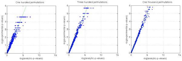
Variation of approximation error at low p-values with number of permutations

To understand how the accuracy of this approximation decays with factors such as dimensionality, sample size and number of permutations we can use the fact that s_j can be expressed as a function of w_j and w^Tw.

$$s_j=f(w_j,{\mathbf{w}}^{\mathbf{T}}\mathbf{w})=\frac{w_j}{{\mathbf{w}}^{\mathbf{T}}\mathbf{w}}$$ (16)

Then if Δw_j is the uncertainity in estimating w_j we can use error propagation theory to deduce:

$${\left(\Delta s_j\right)}^2\approx {\left({\partial }_{w_j}f\right)}^2{\left(\Delta w_j\right)}^2+{\left({{\partial }_{\mathbf{w}}}^{\mathbf{T}}\mathbf{w}f\right)}^2{\left(\Delta {\mathbf{w}}^{\mathbf{T}}\mathbf{w}\right)}^2+crossterms$$ (17)

Ignoring, the higher order terms we get:

$${\left(\frac{\Delta s_j}{s_j}\right)}^2=\left[{\left(\frac{\Delta w_j}{w_j}\right)}^2+{\left(\frac{\Delta {\mathbf{w}}^{\mathbf{T}}\mathbf{w}}{{\mathbf{w}}^{\mathbf{T}}\mathbf{w}}\right)}^2\right]>{\left(\frac{\Delta w_j}{w_j}\right)}^2$$ (18)

Thus the relative error in approximating s_j is larger than that of approximating w_j alone. The above expression provides a relationship between the approximation error on s_j and w_j. The behavior of the approximation error on p-values generated using the w_j (as compared to actual permutations) has been documented in (Gaonkar and Davatzikos, 2013). Any increase in error in approximating components of w will produce a monotonic increase in the approximation error of s_j. Thus, factors such as a lower dimensionality and lower sample size which can increase the approximation error of w_j, automatically lead to a corresponding increase in s_j. Also based on (18) the increase in relative error for s_j will be larger than the corresponding increase in relative error for w_j. Consequently we would expect the error in approximation of the p-value maps to be larger for maps based on s_j as compared to those based on w_j.

4. Discussion

4.1. Contributions

We have investigated a statistic that can be used to understand SVM models using permutation testing. Further we have provided an analytical alternative to computationally intensive permutation testing. The proposed framework provides a statistical p-value based framework for interpretation of SVM models. This makes SVM based multivariate inference as simple to use as VBM based univariate inference and provides a view of the phenomenon under investigation that is complementary to univariate analysis. While the speed up provided by the approximation is important , the fact that the statistics are asymptotically normal is more important. The gaussianity of the proposed statistics, opens up a whole world of statistical properties, tests and analyses predicated on the gaussianity assumption. For instance, the t-test itself assumes a distributional form on the underlying data that is close to normality. This is also true for a whole lot of other results in statistical theory. All of this theory can be brought to bear for understanding SVM models in future work.

4.2. Limitations

The approximation proposed above is ultimately based on the approximation detailed in (Gaonkar and Davatzikos, 2013). Thus it inherits the limitations of (Gaonkar and Davatzikos, 2013). Since the primary motivation here is to interpret SVM models and provide a multivariate analysis tool for clinical studies we have not carried out an investigation into the exact mathematical conditions under which the approximations will fail. However, it is instructive to try and understand where the method will fail with respect to the several assumptions it relies upon.

First, as we have shown in the ‘Quantitative analysis’ section, the relative error of s_j is a monotonic function of relative error of the w_j for j ∈ 1, …d. Hence, based on the trends presented in (Gaonkar and Davatzikos, 2013) one can expect that a) The relative error will decrease with an increase in dimensionality of the data b) The relative error will decrease with an increase in sample size of the data.

A second important facet of the method is the relation between m and d. The application of the central limit theorem in (Gaonkar and Davatzikos, 2013) relies upon m → ∞. The assumption that all samples tend are support vectors seems to apply only when d >> m. In order to further understand this relationship we present here a simple experiment with simulated univariate data. We plot the ratio m/d to the ratio of nSV s/m for simulated univariate data in figure 14. It can be seen from the plot that for m/d > 0.2, less than 95% of samples remain support vectors during permutation tests. This would constitute a substantial deviation from our assumption. Thus, it may not be wise to use the approximation in such a case. Fortunately, for image analysis, the number of voxels in an image (even a downsampled image) is in the range of millions while sample sizes barely touch a few hundreds. Thus, we expect m/d << 0.2 for neuroimaging studies for the most part. However, care must be exercised in applying this approximation when m is too large in comparison to d.

Figure 14.

Plot of adherence to assumption that all samples are support vectors as m gets closer to d

A third limitation relates to the definition of C. The definition of C depends on XX^T)⁻¹. If the inversion fails due to any reason the approximation will cease to work.

A further limitation of the method is that it remains very conservative especially when correcting for family wise error rate using the Bonferroni correction. Note that if we were to use a permutation based method such as (Nichols and Holmes, 2002) for FWER correction we would need to actually perform the permutations. This is because we still cannot model the distribution of the maximae of the margin statistic analytically. Recent work by the authors of (Hinrichs et al., 2013) might offer an insight into analytically modelling these distributions. However, this has not been addressed in our current manuscript. Secondly we have used the simplest form of permutation testing for deriving these results. Machine learning and statistics literature is replete with more intricate forms of these tests (Ojala and Garriga, 2010)(Nichols and Holmes, 2002). Indeed there is an entire literature on permutation testing (Pesarin and Wiley, 2001).

While we think that the scope of the current manuscript is too narrow to address each of these issues, we do hope to address some of them in future work.

5. Conclusion

The motivation behind writing this paper is to provide analysts working on large clinical data a fast, intuitive and easy to use tool for interpreting SVM models and for performing multivariate analysis. While SVMs have been successfully used for diagnostic tasks interpreting what portion of the data is most relevant to the SVM decision has been an open problem. We have attempted to provide a statistical p-value based answer to this question.

The approximation described ensures that we can perform this analyses in time and memory comparable to univariate analyses. The gaussianity of the resulting distributions is significant because it opens up the possibility of application of a large body of statistical literature in the analysis of SVM models. The computational advantage obtained over regular permutation testing is especially significant given that the sheer size of imaging/genetic datasets keeps increasing exponentially due to continuous advancements in the underlying acquisition technology. The increased speed also makes it easier to repeat analyses with different variables and parameters or with the addition or subtraction of data. Additionally, methods like this can be very valuable to data analysis in the burgeoning field of neuroimaging genomics where data dimensionalities and sample sizes are expected to be even larger.

Highlights.

• Support vector machines (SVM) use multivariate imaging information for diagnosis.

• Approximate SVM permutation tests for population statistics

• Improved statistics used for SVM permutation testing

• Fast multivariate inference

• Difference between multivariate and univariate inference

Appendix A. Distribution of SVM weight vectors

In the notation of section 2.1 we can write the hard margin SVM formulation as:

$$\begin{array}{cc}\hfill & mi{n}_{\mathbf{w},b}\frac{1}{2}\parallel \mathbf{w}{\parallel }^2\hfill \\ \hfill & subj.to.y_i({\mathbf{w}}^{\mathbf{T}}{\mathbf{x}}_i+b)\ge 1\hfill \\ \hfill & \forall \in \{1,\dots ,m\}\hfill \end{array}$$ (A.1)

It is required that for the ‘support vectors’ (indexed by l ∈ {1,2, .., n_sv}) we have w^Tx_l + b = y_l ∀l. Now, if all our data were support vectors this would allow us to write the constraints in optimization (A.1) as Xw + Jb = y where J is a column matrix of ones and X is a super long matrix with each row representing one image. For high dimensional medical imaging datasets we investigated most data are support vectors for most permutations (Gaonkar and Davatzikos, 2013). Thus, for most permutations we are actually solving the following simpler optimization instead of (A.1):

$$\begin{array}{cc}\hfill & mi{n}_{\mathbf{w},b}\frac{1}{2}\parallel \mathbf{w}{\parallel }^2\hfill \\ \hfill & subj.to.\mathbf{Xw}+\mathbf{J}b=\mathbf{y}\hfill \end{array}$$ (A.2)

We show next how to derive the dual problem and solve for dual variables (α) and why (α ≠ J). One can use the method of Lagrange multipliers to solve (A.2). We introduce the dual variables α ∈ ℝ^m as is standard procedure to yield the Lagrangian:

$$\mathcal{L}(\mathbf{w},b)=\frac{1}{2}\parallel \mathbf{w}{\parallel }_2^2+{\alpha }^T(\mathbf{Xw}+\mathbf{J}b-y)$$ (A.3)

Setting $\frac{\partial }{\partial \mathbf{w}}\mathcal{L}(\mathbf{b},b)=0,\frac{\partial }{\partial \mathbf{w}}\mathcal{L}(\mathbf{w},b)=0\text{and}\frac{\partial }{\partial \alpha }\mathcal{L}(\mathbf{w},b)=0$, and solving for w yields the following system of equations:

$$\frac{\partial \mathcal{L}}{\partial \mathbf{w}}=0\to \mathbf{w}={\mathbf{X}}^T\alpha ,$$ (A.4)

$$\frac{\partial \mathcal{L}}{\partial b}=0\to {\mathbf{J}}^{\mathbf{T}}\alpha =0,$$ (A.5)

$$\frac{\partial \mathcal{L}}{\partial \alpha }=0\to \mathrm{y}=\mathbf{Xw}+\mathbf{J}b={\mathbf{XX}}^{\mathbf{T}}\alpha +\mathbf{J}b$$ (A.6)

This yields a system of simultaneous equations:

$$\left[\begin{array}{cc}\hfill 0\hfill & \hfill {\mathbf{J}}^T\hfill \\ \hfill \mathbf{J}\hfill & \hfill {\mathbf{XX}}^{\mathbf{T}}\hfill \end{array}\right]\left[\begin{array}{c}\hfill b\hfill \\ \hfill \alpha \hfill \end{array}\right]\left[\begin{array}{c}\hfill 0\hfill \\ \hfill \mathrm{y}\hfill \end{array}\right]$$ (A.7)

Now recall from the derivation of the Woodbury matrix identity that we can compute:

$${\left[\begin{array}{cc}\hfill 0\hfill & \hfill {\mathbf{J}}^T\hfill \\ \hfill \mathbf{J}\hfill & \hfill {\mathbf{XX}}^{\mathbf{T}}\hfill \end{array}\right]}^{-1}$$ (A.8)

as being:

$$\left[\begin{array}{cc}\hfill {(-{\mathbf{J}}^T{\left({\mathbf{XX}}^{\mathbf{T}}\right)}^{-1}\mathbf{J})}^{-1}\hfill & \hfill -{(-{\mathbf{J}}^T{\left({\mathbf{XX}}^{\mathbf{T}}\right)}^{-1}\mathbf{J})}^{-1}{\mathbf{J}}^T{\left({\mathbf{XX}}^{\mathbf{T}}\right)}^{-1}\hfill \\ \hfill -{\left({\mathbf{XX}}^{\mathbf{T}}\right)}^{-1}\mathbf{J}{(-{\mathbf{J}}^T{\left({\mathbf{XX}}^T\right)}^{-1}\mathbf{J})}^{-1}\hfill & \hfill {\left({\mathbf{XX}}^{\mathbf{T}}\right)}^{-1}+{\left({\mathbf{XX}}^{\mathbf{T}}\right)}^{-1}\mathbf{J}{(-{\mathbf{J}}^T{\left({\mathbf{XX}}^{\mathbf{T}}\right)}^{-1}\mathbf{J})}^{-1}{\mathbf{J}}^T{\left({\mathbf{XX}}^{\mathbf{T}}\right)}^{-1}\hfill \end{array}\right]$$

Note that the inversion relies on the assumption that the kernel matrix XX^T is invertible. We can use this inverted form in order to solve for both α and b. Specifically, we can write the dual variables α as:

$$\alpha =[{\left({\mathbf{XX}}^{\mathbf{T}}\right)}^{-1}+{\left({\mathbf{XX}}^{\mathbf{T}}\right)}^{-1}\mathbf{J}{(-{\mathbf{J}}^{\mathbf{T}}{\left({\mathbf{XX}}^{\mathbf{T}}\right)}^{-1}\mathbf{J})}^{-1}{\mathbf{J}}^{\mathbf{T}}{\left({\mathbf{XX}}^{\mathbf{T}}\right)}^{-1}]y$$ (A.9)

These are the dual variables in our formulation. The expression for w then follows from the dual variables as:

$$\mathbf{w}={\mathbf{X}}^{\mathbf{T}}[{\left({\mathbf{XX}}^{\mathbf{T}}\right)}^{-1}+{\left({\mathbf{XX}}^{\mathbf{T}}\right)}^{-1}\mathbf{J}{(-{\mathbf{J}}^{\mathbf{T}}{\left({\mathbf{XX}}^{\mathbf{T}}\right)}^{-1}\mathbf{J})}^{-1}{\mathbf{J}}^{\mathbf{T}}{\left({\mathbf{XX}}^{\mathbf{T}}\right)}^{-1}]y=\mathrm{Cy}$$ (A.10)

where we have defined:

$$\mathrm{C}={\mathbf{X}}^{\mathbf{T}}[{\left({\mathbf{XX}}^{\mathbf{T}}\right)}^{-1}+{\left({\mathbf{XX}}^{\mathbf{T}}\right)}^{-1}\mathbf{J}{(-{\mathbf{J}}^{\mathbf{T}}{\left({\mathbf{XX}}^{\mathbf{T}}\right)}^{-1}\mathbf{J})}^{-1}{\mathbf{J}}^{\mathbf{T}}{\left({\mathbf{XX}}^{\mathbf{T}}\right)}^{-1}]$$ (A.11)

Next we let p denote the fraction of data with label +1 and hypothesize the distribution of y_i to be:

$$Pr(y_i=+1)=pPr(y_i=-1)=1-p$$ (A.12)

This leads to an expected value and variance of y_i:

$$E\left(y_i\right)=2p-1Var\left(y_i\right)=4p-4p^2$$ (A.13)

We can use this to compute the expectation and variance of the components of w using (A.10) as:

$$E\left(w_j\right)=(2p-1)\sum _{i=1}^m{C}_{ij}Var\left(w_j\right)=(4p-4p^2)\sum _{i=1}^m{C}_{ij}^2$$ (A.14)

Note that we may write equation (A.10) as:

$$w_j=\sum _{i=1}^m{C}_{ij}{y}_i=\sum _{i=1}^m{z}_i^j$$ (A.15)

where we have defined a new random variable $z_i^j=C_{ij}{y}_i$ which is linearly dependent on y_i. Since the y_i are subject specific labels we expect them to be independent of each other and we can use the Lyapunov central limit theorem to claim the asymptotic normality on the distributions of w_j. However, application of this theorem requires:

$$\underset{m\to \infty ,d>>m}{\text{lim}}\frac{1}{{\left[\sqrt{\sum _{i=1}^m}Var\left(z_i^j\right)\right]}^{2+\delta }}\sum _{k=1}^m\text{E}\left[\mid z_k^j-{\mu }_k^j{\mid }^{2+\delta }\right]=0forsome\delta >0$$ (A.16)

where $z_i^j=C_{ij}{y}_i$ To apply the Lyapunov CLT, we need the limit to vanish for some δ > 0: We write down the limit for δ = 2 here, as opposed to δ = 1 in the original paper. We do this because the limits are easier to write down and intuit with δ = 2.

$$\underset{m\to \infty ,d>>m}{\text{lim}}\frac{\sum _{k=1}^{m}p\mid C_{kj}-(2p-1)C_{kj}{\mid }^4+(1-p)\mid C_{kj}+(2p-1)C_{kj}{\mid }^4}{\left[\sqrt{(4p-4p^2)\sum _{i=1}^m{C}_{ij}^2}\right]}=0$$ (A.17)

The limit vanishes because the denominator contains cross terms not included in the numerator implying Gaussianity and leading to equation (5).

To see this first note that:

$$\underset{m\to \infty ,d>>m}{\text{lim}}\frac{\sum _{k=1}^{m}p{(2-2p)}^4\mid C_{kj}{\mid }^4+(1-p){\left(2p\right)}^4\mid C_{kj}{\mid }^4}{{\left[\sqrt{(4p-4p^2)\sum _{i=1}^m{C}_{ij}^2}\right]}^4}=0$$ (A.18)

may be broken down to

$$\underset{m\to \infty ,d>>m}{\text{lim}}\frac{\sum _{k=1}^{m}p{(2-2p)}^4\mid C_{kj}{\mid }^4}{{\left[\sqrt{(4p-4p^2)\sum _{i=1}^m{C}_{ij}^2}\right]}^4}+\underset{m\to \infty ,d>>m}{\text{lim}}\frac{\sum _{k=1}^m(1-p){\left(2p\right)}^4\mid C_{kj}{\mid }^4}{{\left[\sqrt{(4p-4p^2)\sum _{i=1}^m{C}_{ij}^2}\right]}^4}=0$$ (A.19)

Since p, 1 − p and 4p − 4p² are constants with respect to m, and the index i is interchangeable with k this boils down to the limit:

$$\underset{m\to \infty ,d>>m}{\text{lim}}\frac{\sum _{k=1}^m\mid {C_{kj}}^4}{{\left(\sum _{k=1}^m{C}_{kj}^2\right)}^{4∕2}}=\underset{m\to \infty ,d>>m}{\text{lim}}\frac{\sum _{k=1}^m{\left(C_{kj}^2\right)}^2}{{\left(\sum _{k=1}^m{C}_{kj}^2\right)}^2}=0\ast$$ (A.20)

For all experiments we performed using several different datasets this limit goes to zero. The intuitive explanation for this is that The binomial expansion of the denominator contains cross terms in addition to the terms in the numerator (a total of m² terms), whereas the numerator contains only m terms. This intuition obviously relies on the assumption that the coefficients $C_{kj}^2$ are of comparable magnitude for different values of k and grow consistently with each other as m grows. But since we already know that:

$$\mathbf{C}={\mathbf{X}}^{\mathbf{T}}[{\left({\mathbf{XX}}^{\mathbf{T}}\right)}^{-1}+\left({\mathbf{XX}}^{\mathbf{T}}\right)-1\mathbf{J}{(-{\mathbf{J}}^{\mathbf{T}}{\left({\mathbf{XX}}^{\mathbf{T}}\right)}^{-1}\mathbf{J})}^{-1}{\mathbf{J}}^{\mathbf{T}}{\left({\mathbf{XX}}^{\mathbf{T}}\right)}^{-1}]$$ (A.21)

At this point note that the Cayley Hamilton theorem gives us for (XX^T)⁻¹

$${\left({\mathbf{XX}}^{\mathbf{T}}\right)}^{-1}=\frac{1}{det\left({\mathbf{XX}}^{\mathbf{T}}\right)}\sum _{s=0}^{m-1}{C}_s{\left({\mathbf{XX}}^{\mathbf{T}}\right)}^s$$ (A.22)

where c_s are the appropriate constants.

Since the terms of XX^T are ultimately quadratic in the X_uv(the elements of the data matrix), the Cayley Hamilton theorem tells us that each term in the inverse can be expressed as a ratio of polynomials whose degree depends on m. This combined with the fact that −J^T(XX^T)⁻¹J is essentially the sum of all terms in (XX^T)⁻¹ allows us to express the elements of C as:

$$C_{kj}=\frac{P_{kj}\left(X_{uv}\right)}{Q\left(X_{uv}\right)}$$ (A.23)

Here P_kj ≠ 0 as long as the all entries in the j^th column of X are not identical (that is we do not deal with the degenerate case where w_j will be 0). The limit , then boils down to:

$$\underset{m\to \infty }{\text{lim}}\frac{\sum _{k=1}^m{\left(P_{kj}^2(X_{uv},m)\right)}^2}{\sum _{k=1}^m{\left(P_{kj}^2(X_{uv},m)\right)}^2}$$ (A.24)

Given a specific value of m, the application of Cayley Hamilton theorem yields a common denominator polynomial Q for all elements of C. For a given m the degrees of the polynomials P_kj are also identical for all values of k and j. This can be easily verified with the use of the matlab symbolic math toolbox or Mathematica.

Since, the P_kj are polynomial functions of the elements of X of an identical degree, we expect them to grow identically with m. That is, P_kj ∈ Θ(g(m, X_uv)). As long as a newly picked sample does not look too different from historical samples (that is assuming exchangeability in X_uv) we may safely assume P_kj ∈ Θ(g(m))

Then, setting a_k = P_kj > 0 with q = 2, under the assumption that a_k ∈ Θ(g(m)) for some function g(m), we look at the limit:

$$\underset{m\to \infty }{\text{lim}}\frac{\sum _{k=1}^m{a}_k^q}{{\left(\sum _{k=1}^m{a}_k\right)}^q}=0$$ (A.25)

To see this, note that the big-Θ notation implies that there exist constants M₁ and M₂ such that M₁g(m) ≤ a_k ≤ M₂g(m).

Then for q¿1:

$$\underset{m\to \infty }{\text{lim}}\frac{\sum _{k=1}^m{a}_k^q}{{\left(\sum _{k=1}^m{a}_k\right)}^q}\le \underset{m\to \infty }{\text{lim}}\frac{m{M}_2^q{\left[g\left(m\right)\right]}^q}{m^q{M}_1^q{\left[g\left(m\right)\right]}^q}=\underset{m\to \infty }{\text{lim}}\frac{1}{m^{q-1}}\frac{M_2^q}{M_1^q}=0$$ (A.26)

Also:

$$\underset{m\to \infty }{\text{lim}}\frac{\sum _{k=1}^m{a}_k^q}{{\left(\sum _{k=1}^m{a}_k\right)}^q}\le \underset{m\to \infty }{\text{lim}}\frac{m{M}_1^q{\left[g\left(m\right)\right]}^q}{m^q{M}_2^q{\left[a\left(m\right)\right]}^q}=\underset{m\to \infty }{\text{lim}}\frac{1}{m^{q-1}}\frac{M_1^q}{M_2^q}=0$$ (A.27)

Then by the squeeze theorem on limits:

$$\underset{m\to \infty }{\text{lim}}\frac{\sum _{k=1}^m{a}_k^q}{{\left(\sum _{k=1}^m{a}_k\right)}^q}=0$$ (A.28)

In summary, if one makes an assumption of exchangeability of the C_kj with respect to the sampling of X, then $C_{kj}^2$ ∈ Θ(g(m)) and we have

$$\underset{m\to \infty }{\text{lim}}\frac{\sum _{k=1}^m{\left(C_{kj}^2\right)}^2}{{\left(\sum _{k=1}^m{C}_{kj}^2\right)}^2}=0$$ (A.29)

As such this assumption allows for a broad range of values of C_kj and seems to be met in our experiments. A more formal treatment surrounding the behavior of this ratio is a topic of research in mathematical statistics, which we feel is beyond the scope of this work on medical image analysis. We refer the interested reader to references (McLeish and O’Brien, 1982; Ladoucette, 2007; Fuchs et al., 2002) where the behavior above ratio has been treated with far more rigor..

References

- Ashburner J, Friston KJ. Voxel-based morphometry–the methods. Neuroimage. 2000;11:805–821. doi: 10.1006/nimg.2000.0582. URL: http://dx.doi.org/10.1006/nimg.2000.0582, doi:10.1006/nimg.2000.0582. [DOI] [PubMed] [Google Scholar]
- Batmanghelich N, Taskar B, Davatzikos C. Generative-discriminative basis learning for medical imaging. Medical Imaging, IEEE Transactions on. 2012;31:51–69. doi: 10.1109/TMI.2011.2162961. doi:10.1109/TMI.2011.2162961. [DOI] [PMC free article] [PubMed] [Google Scholar]
- Benjamini Y, Yekutieli D. The control of the false discovery rate in multiple testing under dependency. Annals of Statistics. 2001;29:1165–1188. [Google Scholar]
- Bühlmann P, Van De Geer S. Statistics for high-dimensional data. Springerverlag Berlin Heidelberg; 2011. [Google Scholar]
- Bunea F, She Y, Ombao H, Gongvatana A, Devlin K, Cohen R. Penalized least squares regression methods and applications to neuroimaging. NeuroImage. 2011;55:1519–1527. doi: 10.1016/j.neuroimage.2010.12.028. URL: http://www.sciencedirect.com/science/article/pii/S1053811910016113, doi:http://dx.doi.org/10.1016/j.neuroimage.2010.12.028. [DOI] [PMC free article] [PubMed] [Google Scholar]
- Burges CJC. A tutorial on support vector machines for pattern recognition. Data Mining and Knowledge Discovery. 1998;2:121–167. URL: http://citeseerx.ist.psu.edu/viewdoc/summary?doi=10.1.1.117.3731. [Google Scholar]
- Casella G, Berger RL. Statistical inference. Vol. 2. Duxbury Pacific Grove; CA: 2002. [Google Scholar]
- Chung MK. Computational Neuroanatomy: The Methods. World Scientific Publishing Company; 2012. [Google Scholar]
- Craddock RC, Holtzheimer PE, 3rd, Hu XP, Mayberg HS. Disease state prediction from resting state functional connectivity. Magn Reson Med. 2009;62:1619–1628. doi: 10.1002/mrm.22159. URL: http://dx.doi.org/10.1002/mrm.22159, doi:10.1002/mrm.22159. [DOI] [PMC free article] [PubMed] [Google Scholar]
- Cuingnet R, Rosso C, Chupin M, Lehéricy S, Dormont D, Benali H, Samson Y, Colliot O. Spatial regularization of svm for the detection of diffusion alterations associated with stroke outcome. Medical image analysis. 2011;15:729–737. doi: 10.1016/j.media.2011.05.007. [DOI] [PubMed] [Google Scholar]
- Davatzikos C. Why voxel-based morphometric analysis should be used with great caution when characterizing group differences. Neuroimage. 2004;23:17–20. doi: 10.1016/j.neuroimage.2004.05.010. URL: http://dx.doi.org/10.1016/j.neuroimage.2004.05.010, doi:10.1016/j.neuroimage.2004.05.010. [DOI] [PubMed] [Google Scholar]
- Davatzikos C, Bhatt P, Shaw LM, Batmanghelich KN, Trojanowski JQ. Prediction of mci to ad conversion, via mri, csf biomarkers, and pattern classification. Neurobiol Aging. 2011;32:2322.e19–2322.e27. doi: 10.1016/j.neurobiolaging.2010.05.023. URL: http://dx.doi.org/10.1016/j.neurobiolaging.2010.05.023, doi:10.1016/j.neurobiolaging.2010.05.023. [DOI] [PMC free article] [PubMed] [Google Scholar]
- Davatzikos C, Genc A, Xu D, Resnick SM. Voxel-based morphometry using the ravens maps: methods and validation using simulated longitudinal atrophy. Neuroimage. 2001;14:1361–1369. doi: 10.1006/nimg.2001.0937. URL: http://dx.doi.org/10.1006/nimg.2001.0937, doi:10.1006/nimg.2001.0937. [DOI] [PubMed] [Google Scholar]
- De Martino F, Valente G, Staeren N, Ashburner J, Goebel R, Formisano E. Combining multivariate voxel selection and support vector machines for mapping and classification of fmri spatial patterns. Neuroimage. 2008;43:44–58. doi: 10.1016/j.neuroimage.2008.06.037. URL: http://dx.doi.org/10.1016/j.neuroimage.2008.06.037, doi:10.1016/j.neuroimage.2008.06.037. [DOI] [PubMed] [Google Scholar]
- Etzel JA, Zacks JM, Braver TS. Searchlight analysis: promise, pitfalls, and potential. NeuroImage; 2013. [DOI] [PMC free article] [PubMed] [Google Scholar]
- Fan Y, Shen D, Gur RC, Gur RE, Davatzikos C. Compare: classification of morphological patterns using adaptive regional elements. IEEE Trans Med Imaging. 2007;26:93–105. doi: 10.1109/TMI.2006.886812. URL: http://dx.doi.org/10.1109/TMI.2006.886812, doi:10.1109/TMI.2006.886812. [DOI] [PubMed] [Google Scholar]
- Friston KJ. Eigenimages and multivariate analyses. Human Brain Function; 1997. [Google Scholar]
- Friston KJ, Frith CD, Frackowiak RS, Turner R. Characterizing dynamic brain responses with fmri: a multivariate approach. Neuroimage. 1995;2:166–172. doi: 10.1006/nimg.1995.1019. [DOI] [PubMed] [Google Scholar]
- Friston KJ, Frith CD, Liddle PF, Frackowiak RS. Functional connectivity: the principal-component analysis of large (pet) data sets. J Cereb Blood Flow Metab. 1993;13:5–14. doi: 10.1038/jcbfm.1993.4. URL: http://dx.doi.org/10.1038/jcbfm.1993.4, doi:10.1038/jcbfm.1993.4. [DOI] [PubMed] [Google Scholar]
- Fuchs A, Joffe A, Teugels J. Expectation of the ratio of the sum of squares to the square of the sum: exact and asymptotic results. Theory of Probability & Its Applications. 2002;46:243–255. [Google Scholar]
- Fujikoshi Y, Himeno T, Wakaki H. Asymptotic results of a high dimensional manova test and power comparison when the dimension is large compared to the sample size. J. Japan Statist. Soc. 2004;34:19–26. [Google Scholar]
- Gaonkar B, Davatzikos C. Deriving statistical significance maps for svm based image classification and group comparisons; Proceedings of the 15th international conference on Medical Image Computing and Computer-Assisted Intervention - Volume Part I; Springer-Verlag, Berlin, Heidelberg. 2012. pp. 723–730. [DOI] [PMC free article] [PubMed] [Google Scholar]
- Gaonkar B, Davatzikos C. Analytic estimation of statistical significance maps for support vector machine based multi-variate image analysis and classification. NeuroImage . 2013 doi: 10.1016/j.neuroimage.2013.03.066. [DOI] [PMC free article] [PubMed] [Google Scholar]
- Golland P, Fischl B. Information processing in medical imaging. Springer; 2003. Permutation tests for classification: towards statistical significance in image-based studies; pp. 330–341. [DOI] [PubMed] [Google Scholar]
- Guyon I, Weston J, Barnhill S, Vapnik V. Gene selection for cancer classification using support vector machines. Machine learning. 2002;46:389–422. [Google Scholar]
- Hardin D, Tsamardinos I, Aliferis CF. A theoretical characterization of linear svm-based feature selection; Proceedings of the twenty-first international conference on Machine learning; ACM. 2004. p. 48. [Google Scholar]
- Hinrichs C, Ithapu V, Sun Q, Johnson SC, Singh V. Speeding up permutation testing in neuroimaging. Advances in Neural Information Processing Systems. 2013:890–898. [PMC free article] [PubMed] [Google Scholar]
- Hsing T, Attoor S, Dougherty E. Relation between permutation-test p values and classifier error estimates. Machine Learning. 2003;52:11–30. [Google Scholar]
- Kearns MJ, Vazirani UV. An introduction to computational learning theory. MIT press; 1994. [Google Scholar]
- Kherif F, Poline JB, Flandin G, Benali H, Simon O, Dehaene S, Worsley KJ. Multivariate model specification for fmri data. NeuroImage. 2002;16:1068–1083. doi: 10.1006/nimg.2002.1094. [DOI] [PubMed] [Google Scholar]
- Kim SG, Chung MK, Schaefer SM, van Reekum C, Davidson RJ. Sparse shape representation using the laplace-beltrami eigenfunctions and its application to modeling subcortical structures. Mathematical Methods in Biomedical Image Analysis (MMBIA) 2012:25–32. doi: 10.1109/MMBIA.2012.6164736. 2012 IEEE Workshop on, IEEE. [DOI] [PMC free article] [PubMed] [Google Scholar]
- Klöppel S, Stonnington CM, Chu C, Draganski B, Scahill RI, Rohrer JD, Fox NC, Jack CR, Ashburner J, Frackowiak RS. Automatic classification of mr scans in alzheimer’s disease. Brain. 2008;131:681–689. doi: 10.1093/brain/awm319. [DOI] [PMC free article] [PubMed] [Google Scholar]
- Ladoucette SA. Asymptotic behavior of the moments of the ratio of the random sum of squares to the square of the random sum. Statistics & probability letters. 2007;77:1021–1033. [Google Scholar]
- McIntosh A, Bookstein F, Haxby JV, Grady C. Spatial pattern analysis of functional brain images using partial least squares. Neuroimage. 1996;3:143–157. doi: 10.1006/nimg.1996.0016. [DOI] [PubMed] [Google Scholar]
- McKeown MJ, Sejnowski TJ. Independent component analysis of fmri data: examining the assumptions. Hum Brain Mapp. 1998;6:368–372. doi: 10.1002/(SICI)1097-0193(1998)6:5/6<368::AID-HBM7>3.0.CO;2-E. [DOI] [PMC free article] [PubMed] [Google Scholar]
- McLeish D, O’Brien G. The expected ratio of the sum of squares to the square of the sum. The Annals of Probability. 1982:1019–1028. [Google Scholar]
- Mingoia G, Wagner G, Langbein K, Maitra R, Smesny S, Dietzek M, Burmeister HP, Reichenbach JR, Schlsser RGM, Gaser C, Sauer H, Nenadic I. Default mode network activity in schizophrenia studied at resting state using probabilistic ica. Schizophr Res. 2012 doi: 10.1016/j.schres.2012.01.036. URL: http://dx.doi.org/10.1016/j.schres.2012.01.036, doi:10.1016/j.schres.2012.01.036. [DOI] [PubMed]
- Morrison DF. Multivariate statistical methods. 1967 [Google Scholar]
- Mouro-Miranda J, Bokde ALW, Born C, Hampel H, Stetter M. Classifying brain states and determining the discriminating activation patterns: Support vector machine on functional mri data. Neuroimage. 2005;28:980–995. doi: 10.1016/j.neuroimage.2005.06.070. URL: http://dx.doi.org/10.1016/j.neuroimage.2005.06.070, doi:10.1016/j.neuroimage.2005.06.070. [DOI] [PubMed] [Google Scholar]
- Nichols TE, Holmes AP. Nonparametric permutation tests for functional neuroimaging: a primer with examples. Hum Brain Mapp. 2002;15:1–25. doi: 10.1002/hbm.1058. [DOI] [PMC free article] [PubMed] [Google Scholar]
- Ojala M, Garriga GC. Permutation tests for studying classifier performance. The Journal of Machine Learning Research. 2010;11:1833–1863. [Google Scholar]
- Perlbarg V, Bellec P, Anton JL, Pélégrini-Issac M, Doyon J, Benali H. Corsica: correction of structured noise in fmri by automatic identification of ica components. Magnetic resonance imaging. 2007;25:35–46. doi: 10.1016/j.mri.2006.09.042. [DOI] [PubMed] [Google Scholar]
- Pesarin F, Wiley J. Multivariate permutation tests: with applications in biostatistics. Wiley Chichester; 2001. 240. [Google Scholar]
- Pham DL, Prince JL. Adaptive fuzzy segmentation of magnetic resonance images. IEEE Trans Med Imaging. 1999;18:737–752. doi: 10.1109/42.802752. URL: http://dx.doi.org/10.1109/42.802752, doi:10.1109/42.802752. [DOI] [PubMed] [Google Scholar]
- Rao A, Garg R, Cecchi G. A spatio-temporal support vector machine searchlight for fmri analysis; Biomedical Imaging: From Nano to Macro, 2011 IEEE International Symposium on; 2011. pp. 1023–1026. doi:10.1109/ISBI.2011. 5872575. [Google Scholar]
- Rasmussen PM, Hansen LK, Madsen KH, Churchill NW, Strother SC. Model sparsity and brain pattern interpretation of classification models in neuroimaging. Pattern Recognition. 2012;45:2085–2100. doi: http://dx.doi.org/10.1016/j.patcog.2011.09.011. [Google Scholar]
- Rasmussen PM, Madsen KH, Lund TE, Hansen LK. Visualization of nonlinear kernel models in neuroimaging by sensitivity maps. NeuroImage. 2011;55:1120–1131. doi: 10.1016/j.neuroimage.2010.12.035. [DOI] [PubMed] [Google Scholar]
- Searle SR. Linear models. John Wiley & Sons; 2012. [Google Scholar]
- Sled JG, Zijdenbos AP, Evans AC. A nonparametric method for automatic correction of intensity nonuniformity in mri data. IEEE Trans Med Imaging. 1998;17:87–97. doi: 10.1109/42.668698. URL: http://dx.doi.org/10.1109/42.668698, doi:10.1109/42.668698. [DOI] [PubMed] [Google Scholar]
- Smith SM. Fast robust automated brain extraction. Hum Brain Mapp. 2002;17:143–155. doi: 10.1002/hbm.10062. URL: http://dx.doi.org/10.1002/hbm.10062, doi:10.1002/hbm.10062. [DOI] [PMC free article] [PubMed] [Google Scholar]
- Smith SM, Jenkinson M, Woolrich MW, Beckmann CF, Behrens TE, Johansen-Berg H, Bannister PR, De Luca M, Drobnjak I, Flitney DE, et al. Advances in functional and structural mr image analysis and implementation as fsl. Neuroimage. 2004;23:S208–S219. doi: 10.1016/j.neuroimage.2004.07.051. [DOI] [PubMed] [Google Scholar]
- Srivastava MS, Du M. A test for the mean vector with fewer observations than the dimension. Journal of Multivariate Analysis. 2008;99:386–402. [Google Scholar]
- Stone J, Porrill J, Porter N, Wilkinson I. Spatiotemporal independent component analysis of event-related fmri data using skewed probability density functions. NeuroImage. 2002;15:407–421. doi: 10.1006/nimg.2001.0986. [DOI] [PubMed] [Google Scholar]
- Svensén M, Kruggel F, Benali H. Ica of fmri group study data. NeuroImage. 2002;16:551–563. doi: 10.1006/nimg.2002.1122. [DOI] [PubMed] [Google Scholar]
- Van De Ville D, Blu T, Unser M. Integrated wavelet processing and spatial statistical testing of fmri data. NeuroImage. 2004;23:1472–1485. doi: 10.1016/j.neuroimage.2004.07.056. [DOI] [PubMed] [Google Scholar]
- Van De Ville D, Seghier ML, Lazeyras F, Blu T, Unser M. Wspm: Wavelet-based statistical parametric mapping. NeuroImage. 2007;37:1205–1217. doi: 10.1016/j.neuroimage.2007.06.011. [DOI] [PubMed] [Google Scholar]
- Vapnik VN. The nature of statistical learning theory. Springer-Verlag New York, Inc.; New York, NY, USA: 1995. [Google Scholar]
- Vemuri P, Gunter JL, Senjem ML, Whitwell JL, Kantarci K, Knopman DS, Boeve BF, Petersen RC, Jack CR., Jr Alzheimer’s disease diagnosis in individual subjects using structural mr images: validation studies. Neuroimage. 2008;39:1186–1197. doi: 10.1016/j.neuroimage.2007.09.073. URL: http://dx.doi.org/10.1016/j.neuroimage.2007.09.073, doi:10.1016/j.neuroimage.2007.09.073. [DOI] [PMC free article] [PubMed] [Google Scholar]
- Wang Z, Childress AR, Wang J, Detre JA. Support vector machine learning-based fmri data group analysis. Neuroimage. 2007;36:1139–1151. doi: 10.1016/j.neuroimage.2007.03.072. URL: http://dx.doi.org/10.1016/j.neuroimage.2007.03.072, doi:10.1016/j.neuroimage.2007.03.072. [DOI] [PMC free article] [PubMed] [Google Scholar]
- Xiao Y, Rao R, Cecchi G, Kaplan E. Improved mapping of information distribution across the cortical surface with the support vector machine. Neural Netw. 2008;21:341–348. doi: 10.1016/j.neunet.2007.12.022. URL: http://dx.doi.org/10.1016/j.neunet.2007.12.022, doi:10.1016/j.neunet.2007.12.022. [DOI] [PMC free article] [PubMed] [Google Scholar]
- Xu L, Groth KM, Pearlson G, Schretlen DJ, Calhoun VD. Source-based morphometry: the use of independent component analysis to identify gray matter differences with application to schizophrenia. Hum Brain Mapp. 2009;30:711–724. doi: 10.1002/hbm.20540. URL: http://dx.doi.org/10.1002/hbm.20540, doi:10.1002/hbm.20540. [DOI] [PMC free article] [PubMed] [Google Scholar]
- Yushkevich PA, Piven J, Cody Hazlett H, Gimpel Smith R, Ho S, Gee JC, Gerig G. User-guided 3D active contour segmentation of anatomical structures: Significantly improved efficiency and reliability. Neuroimage. 2006;31:1116–1128. doi: 10.1016/j.neuroimage.2006.01.015. [DOI] [PubMed] [Google Scholar]
- Zou H, Hastie T. Regularization and variable selection via the elastic net. Journal of the Royal Statistical Society: Series B (Statistical Methodology) 2005;67:301–320. [Google Scholar]