Abstract
Epidemiological studies around the world have reported that fine particulate matter (PM2.5) is closely associated with human health. The distribution of PM2.5 concentrations is influenced by multiple geographic and socioeconomic factors. Using a remote-sensing-derived PM2.5 dataset, this paper explores the relationship between PM2.5 concentrations and meteorological parameters and their spatial variance in China for the period 2001–2010. The spatial variations of the relationships between the annual average PM2.5, the annual average precipitation (AAP), and the annual average temperature (AAT) were evaluated using the Geographically Weighted Regression (GWR) model. The results indicated that PM2.5 had a strong and stable correlation with meteorological parameters. In particular, PM2.5 had a negative correlation with precipitation and a positive correlation with temperature. In addition, the relationship between the variables changed over space, and the strong negative correlation between PM2.5 and the AAP mainly appeared in the warm temperate semihumid region and northern subtropical humid region in 2001 and 2010, with some localized differences. The strong positive correlation between the PM2.5 and the AAT mainly occurred in the mid-temperate semiarid region, the humid, semihumid, and semiarid warm temperate regions, and the northern subtropical humid region in 2001 and 2010.
1. Introduction
Many epidemiological studies have shown that long-term exposure to outdoor air pollution could increase the risk of acute and chronic health effects [1]. Fine particles (PM2.5, i.e., particles with aerodynamic diameters of less than 2.5 μm), which are the main air pollutants, continue to pose significant threats to health worldwide, especially in developing countries. Chronic exposure to PM2.5 has negative effects on human health, including increased morbidity from respiratory problems, cardiovascular problems, and lung cancer [2–4]. Some epidemiological studies have also reported that children have a high susceptibility to respiratory illness when exposed to long-term air pollution due to their developing bodies and immature lungs [5, 6]. In China, the air quality has worsened due to the rapid social and economic development in recent years [7, 8], and more attention has been focused on studies of PM2.5. Therefore, long-term PM2.5 concentration monitoring and accurate estimations of PM2.5 concentrations have become crucial to epidemiological research.
In recent years, the application of satellite remote sensing to air quality research [9, 10], especially the application of aerosol optical depth (AOD) to assessing surface air quality [11], has greatly promoted the estimates of ground-level PM2.5 concentrations. Previous studies have established a positive relationship between observed PM2.5 concentrations and AOD [12–14]. Kumar et al. [15] and Schäfer et al. [16] examine the relationship between PM2.5 and AOD using linear regression. Hu [17] also used Geographically Weighted Regression (GWR) to establish a local relationship between PM2.5 and AOD. Many researchers predicted the surface PM2.5 concentration by using the relationship between PM2.5 and AOD [17, 18].
Local meteorological information can optimize the relationship between AOD and PM2.5 [19, 20], and adoption of meteorological information in a model can significantly improve the model's predictability [21]. Paciorek et al. [22] estimated surface PM2.5 concentrations with the predictive variables of AOD and meteorological parameters. van Donkelaar et al. [11] used a global chemical transport model with meteorological information to simulate the factors that affect the relationship between AOD and PM2.5 and to produce a map of global, annually averaged, remotely sensed PM2.5 concentrations for November 2000–October 2002. Based on the methods of Liu et al. [18], van Donkelaar et al. successfully developed a global satellite-based estimate of surface PM2.5 using meteorological datasets [23]. However, for meteorological information, previous studies usually focused on the planetary boundary layer and relative humidity as key factors that affect the relationship between PM2.5 and AOD [21, 22].
In China, the climate exhibits significant differences due to the country's vastness. Figure 1 shows the climate zones in China [24]. The regions to the right of the red line in Figure 1 are the major economic zones in China, and the PM2.5 in these regions that have high populations, high GDP, and large urban areas has become more serious than that in the regions to the left of the line [25]. Many recent studies also note the association between PM10 and meteorological factors based on the ordinary least squares (OLS) method at locations in China [26, 27]. However, the relationship between PM2.5 and meteorological factors usually exhibits differences in various regions. It is necessary to evaluate the spatial variation of those relationships in China to improve the understanding of air quality and epidemiological studies.
Figure 1.
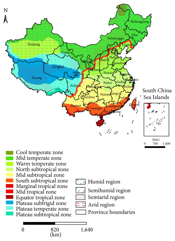
Map of climate zones in China.
The objective of this paper is to explore the relationship between PM2.5 concentrations and meteorological parameters and the associated spatial variance of the relationship in China based on new, long-term raster data. The annual average PM2.5 gridded data, annual average precipitation (AAP) gridded data, and annual average temperature (AAT) gridded data for the period 2001–2010 were used in this study. The spatial variation of the correlations between the PM2.5 concentrations, the AAP, and the AAT were analyzed using the GWR method.
2. Material and Methods
2.1. PM2.5 Data
The global annual average PM2.5 gridded datasets for the period 2001–2010 [28] were downloaded from the website of the Socioeconomic Data and Applications Center (SEDAC). Each data file had a resolution of 0.5° × 0.5°, and all PM2.5 concentrations, which were in micrograms per cubic meter (μg/m3), were multiplied by 1,000.
Based on the work of van Donkelaar et al. [23], researchers of Battelle Memorial Institute developed a method to estimate annual average surface PM2.5 concentrations from AOD. van Donkelaar et al. [23] applied a conversion factor that accounts for the spatiotemporal relationship between PM2.5 and AOD to estimate the ground-level concentration of dry 24-hour PM2.5. The conversion factor in these datasets was treated as constant during 2001–2010 after minor processing; a relative humidity of 50% was used. The PM2.5 concentrations in each grid cell were calculated by multiplying the satellite AOD and the monthly mean conversion factors. Finally, the monthly estimates over each year were averaged to obtain the annual average surface PM2.5 concentrations [28]. Compared with the grids produced by van Donkelaar et al. [23], the global estimated PM2.5 concentrations from these datasets may have some systematic biases over some regions, such as India and counties in the Sahel, North Africa, and the Arabian peninsula. The bias may be induced by the difficulties of AOD retrievals over sandy surfaces or by the application of the conversion factors [28]. The datasets we used in this paper (China region) are hardly affected by that.
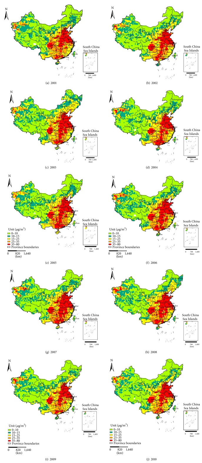
The China annual average PM2.5 gridded datasets for the period 2001–2010 were extracted by ArcGIS software and were transformed to the same coordinate system as the meteorological datasets. Figure 2 shows the estimated distribution of the PM2.5 concentrations in China from 2001 to 2010 according to the WHO air quality guidelines and interim targets [29].
Figure 2.
The estimated distribution of PM2.5 concentrations in China from (a) 2001 to (j) 2010 (classified according to the WHO air quality guidelines and interim targets).
2.2. Meteorological Data
The meteorological datasets used in this paper, including the AAP data and AAT data for the period 2001–2010, were provided by the Resources and Environmental Scientific Data Center (RESDC), Chinese Academy of Sciences, and the China Meteorological Administration (CMA). The datasets were in raster format (ArcGIS GRID format) with a spatial resolution of 1 km.
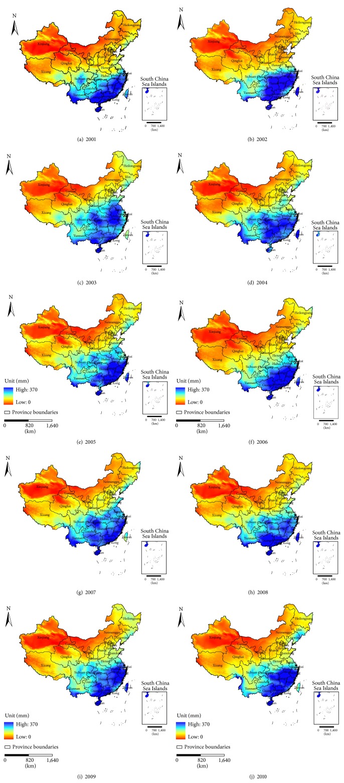
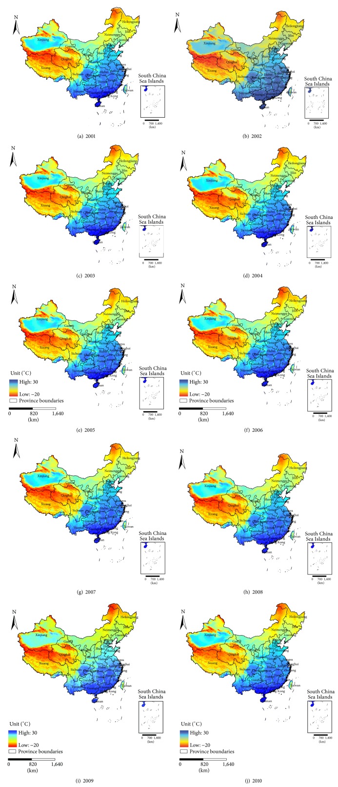
Figures 3 and 4 show the distribution of the AAP and AAT in China for the period 2001–2010.
Figure 3.
The AAP in China for the period (a) 2001–(j) 2010.
Figure 4.
The AAT in China for the period (a) 2001–(j) 2010.
2.3. Methodology
The spatial variance of the relationship between the PM2.5 concentrations and meteorological parameters in China was calculated using the following steps.
Step 1. Evaluate the relationships between the PM2.5 concentrations, AAP, and AAT based on multiple linear regression (MLR) with data of 333 prefectures [30] in China for the period 2001–2010.
Step 2. Use the GWR method to explore the spatial variation of the relationship between the PM2.5 concentrations, AAP, and AAT for 2001 and 2010.
Based on OLS, Fotheringham et al. [31] developed a method to explore spatial heterogeneity by building a local regression model. The GWR model embeds the spatial locations in regression parameters and considers the local estimates of the parameters. The GWR model can show the influence of independent variables on dependent variables with the locations' changes and the spatial heterogeneity of the relationship between an independent variable and dependent variable [32]. Due to the special characteristics of the GWR, it was adopted in this paper to indicate the spatial variance of the relationship between the PM2.5 concentrations, AAP, and AAT.
The global regression model can be expressed as
| (1) |
where (u i, v i) is the spatial coordinate of sample point i and β k(u i, v i) is the regression coefficient of sample point i. ε i is the random error of the independent distribution, which is usually assumed to obey a normal distribution. If β k(u 1, v 1) = β k(u 2, v 2) = ⋯β k(u n, v n), then the model will be changed into an OLS model [33].
Bandwidth, which controls the degree of smoothing, is an important parameter for GWR. There are two automatic methods for finding the bandwidth: CV, which minimizes a cross-validation (CV) function, and AIC, which minimizes the Akaike information criterion (AIC) [33]. In this paper, we chose an adaptive kernel by considering the spatial configuration of the features, and we found the bandwidth by minimizing the corrected Akaike information criterion value as it is less biased compared with AIC [34].
3. Results
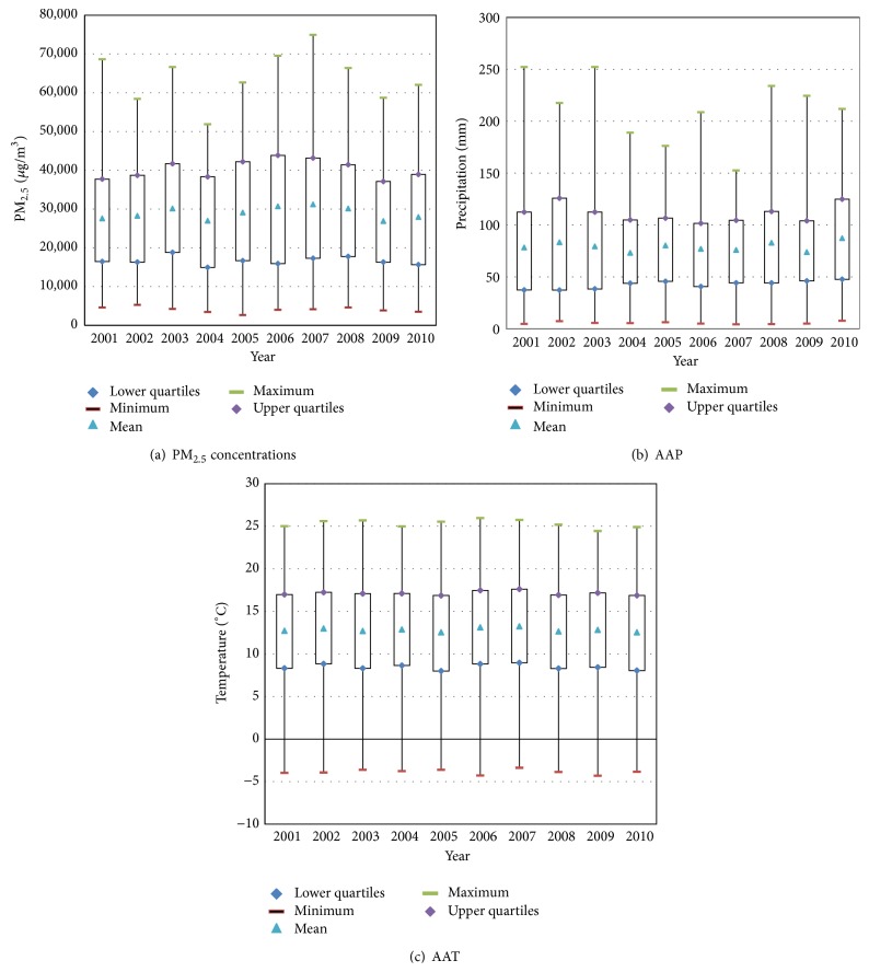
Figure 5 shows the summary statistics of the variables.
Figure 5.
Maps of the summary statistics for the (a) annual average PM2.5, (b) AAP, and (c) AAT.
Based on the above-mentioned maps, we can see the spatial characteristics of the AAP and AAT and the summary statistics of the PM2.5, AAP, and AAT in China for the period 2001–2010. The values of the PM2.5 concentrations, AAP, and AAT during the ten years remained at approximately 28 μg/m3, 79 mm, and 12.79°C, respectively. Thus, the MLR model was first applied to study the correlation between the PM2.5 concentrations and the two meteorological factors. Then, the GWR model was used for evaluating the spatial variation of the relationship between the AAP and AAT in 2001 and 2010.
3.1. Correlation between the PM2.5 Concentrations and Meteorological Parameters
We developed the MLR model based on the data of 333 prefectures in China using SPSS. Table 1 shows the results of the model from 2001 to 2010. Based on the results of the MLR, the R value reached a maximum of 0.75 in 2001 and a minimum of 0.62 in 2009, with a mean value of 0.688; these results indicate a good and stable correlation between the PM2.5 and meteorological parameters in China during 2001–2010. The function for each year also denoted a negative correlation between the PM2.5 concentrations and AAP and a positive correlation between the PM2.5 concentrations and AAT over the period.
Table 1.
The results of the MLR between the PM2.5 concentrations and meteorological parameters from 2001 to 2010 (N = 333).
| Year | Dependent variable (y) | Independent variable | R | The function* | |
|---|---|---|---|---|---|
| x 1 | x 2 | ||||
| 2001 | PM2.5
concentrations |
AAP | AAT | 0.75 | y = −173.89x 1 + 2448.35x 2 + 10080.71 |
| 2002 | 0.67 | y = −134.55x 1 + 2156.00x 2 + 11490.86 | |||
| 2003 | 0.68 | y = −204.51x 1 + 2582.41x 2 + 13435.09 | |||
| 2004 | 0.72 | y = −78.11x 1 + 1879.51x 2 + 8523.51 | |||
| 2005 | 0.70 | y = −118.68x 1 + 2228.16x 2 + 10684.55 | |||
| 2006 | 0.71 | y = −196.71x 1 + 2718.83x 2 + 10189.49 | |||
| 2007 | 0.68 | y = −228.57x 1 + 2747.42x 2 + 12190.28 | |||
| 2008 | 0.69 | y = −188.33x 1 + 2649.73x 2 + 12271.67 | |||
| 2009 | 0.62 | y = −97.78x 1 + 1750.89x 2 + 11694.93 | |||
| 2010 | 0.66 | y = −147.55x 1 + 2257.13x 2 + 12510.72 | |||
*The functions were valid because they all passed the F-test, and all the regression coefficients passed the t-test (at the level of 0.05).
The variance inflation factor (VIF) was used for detecting the existence of the colinearity problem among the indicators via SPSS software. The VIF values of the AAP and AAT were both 2.431 for 2001 and 2.203 for the year 2010. A colinearity problem does not exist among the variables because the VIF values are less than 10 [35].
3.2. The Spatial Variation of the Identified Relationship
In the reports of GWR, we obtained the R 2 and the adjusted R 2 of the two years, that is, 0.784 and 0.781, respectively, for 2001 and 0.782 and 0.780, respectively, for 2010. The adjusted R 2 values for both of the years were better than the values obtained in the MLR models. The means of the local R 2 for 2001 and 2010 were 0.50 and 0.49, respectively. The values for the two years were very similar, which indicates the goodness-of-fit of the models for both of the years.
Figures 6 and 7 show the spatial variation of the relationship between the PM2.5 concentrations and meteorological parameters in 2001 and 2010. Based on the method of Leung et al. [36], in this study, we calculated the f = V GWR/RSSGWR (where V GWR is the variance of the coefficients and RSSGWR is the residual sum of squares), which is tested as an f statistic to examine the spatial nonstability of the regression coefficients of each variable using an F-test. The ratios between the f and the corresponding degrees of freedom for each variable in both years were all larger than the critical value at the level of 0.05; thus, the spatial variation of the regression coefficients of the variables was nonstationary.
Figure 6.
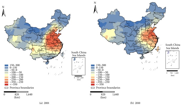
Maps of the local coefficients of the AAP for (a) 2001 and (b) 2010.
Figure 7.
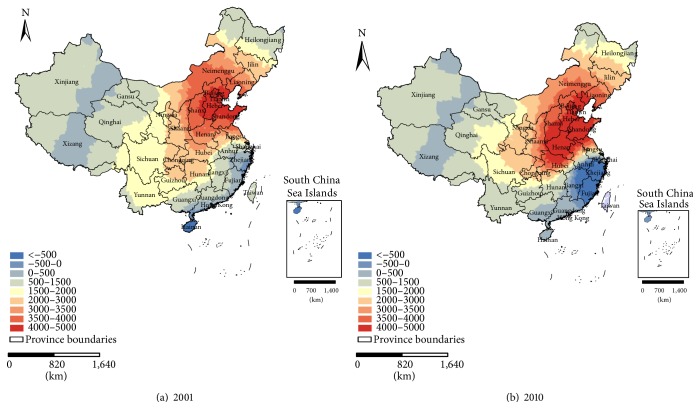
Maps of the local coefficients of the AAT for (a) 2001 and (b) 2010.
Figure 6 shows the local coefficients of the AAP for 2001 and 2010. In general, the local coefficients in 2001 indicate that the influence of the AAP on the PM2.5 varied considerably over the entire country, with a west-east orientation; approximately 83.8% of the study area exhibits a negative correlation between the PM2.5 concentrations and the AAP. The strong correlations with the coefficients below −200 mainly appeared in the warm temperate semihumid region and in the east-central northern subtropical humid region; they rarely emerged in the warm temperate semiarid region or northeast of the mid-subtropical humid region (Figure 1), which includes Beijing, Tianjin, Shanghai, Shandong, Henan, Anhui, Jiangsu, and Zhejiang Provinces and most of Shaanxi, Shanxi, Hebei, Hubei, Hunan, Jiangxi, and Fujian Provinces. In 2010, the overall map is similar to that in 2001, and the influence varies with a west-east orientation. However, the correlations declined in some regions, and only 68.9% of the study area revealed a negative correlation. The strong correlations in 2010 mainly appeared to the southeast of the warm temperate semihumid region and in the east-central area of the northern subtropical humid region; they rarely emerged northeast of the mid-subtropical humid region (Figure 1), which includes Shanghai and Jiangsu Provinces and most of Shandong, Henan, Hubei, Anhui, and Zhejiang Provinces. Compared with 2001, the regions with strong correlations between the PM2.5 and AAP were reduced in 2010. Further, in the regions of Yunnan, Guizhou, Sichuan, and Guangxi, the sign of the local coefficient changed by 2010 and may be a consequence of extreme drought and climate change [37, 38].
Figure 7 shows the local coefficients of the AAT for 2001 and 2010. In general, the local coefficients of 2001 indicate that the influence of the AAT on the PM2.5 varies considerably over the entire country; approximately 98.8% of the study area reveals a positive correlation between the PM2.5 concentrations and the AAT. This finding remarkably agrees with the result obtained from the MLR model. The strong correlations with the coefficients above 3,000 mainly appeared in the mid-temperate semiarid region, the humid, semihumid and semiarid warm temperate regions, and the central area of the northern subtropical humid region; they rarely emerged northeast of the northern subtropical humid region, northeast of the mid-temperate arid region, or south of the humid and semihumid areas of the mid-temperate regions (Figure 1), which include Beijing, Tianjin, Hebei, Shandong, and Shanxi Provinces and most of Liaoning, Neimenggu, Shaanxi, Henan, Hubei, Anhui, and Jiangsu Provinces. Much like the situation in 2001, in 2010, the relationship between the PM2.5 and the AAT varied over space; approximately 89.7% of the study area exhibited a positive correlation. The strong correlations mainly appeared in the mid-temperate semiarid region, the humid, semihumid, and semiarid warm temperate regions, and the central and northeastern areas of the northern subtropical humid region; they rarely emerged in the northwestern mid-subtropical humid region, the northeastern mid-temperate arid region, the southern mid-temperate humid region and the southern mid-temperate semihumid region (Figure 1), which include Beijing, Tianjin, Liaoning, Hebei, Shandong, Henan, and Shanxi Provinces and most of Chongqing, Jilin, Neimenggu, Shaanxi, Hubei, Anhui, and Jiangsu Provinces. Although areas with a positive correlation decreased compared to 2001, the regions with a strong relationship increased in 2010, especially in the regions with coefficients above 4,000. Additionally, the sign of the local coefficient changed in a few regions along the southeastern coast in 2010.
4. Discussion
It was reported that inclusion of AOD and meteorological fields can significantly improve a model's predictability of surface PM2.5 concentrations [19, 21]. Hu et al. [39] built the GWR model to predict the PM2.5 concentrations in the Southeast USA, and Tian and Chen [40] also developed a new model to predict the PM2.5 concentrations utilizing satellite observations, assimilated meteorological fields, and ground-based meteorological measurements in Pennsylvania, USA. As mentioned above, PM2.5 had a strong and stable correlation with meteorological parameters over most of China. Figure 8 shows the values of the standardized residual (StdResid) for 2001 and 2010 obtained from the GWR model. Regions with StdResid values in the range of −2.5 to 2.5 composed 97.9% (2001) and 96.8% (2010) of the entire country and indicate a better predictive ability for PM2.5 concentrations. Although the strength of the correlation between the PM2.5 and meteorological parameters varied over space, the parameters are expected to be good predictive variables for estimating PM2.5 concentrations when combined with AOD.
Figure 8.
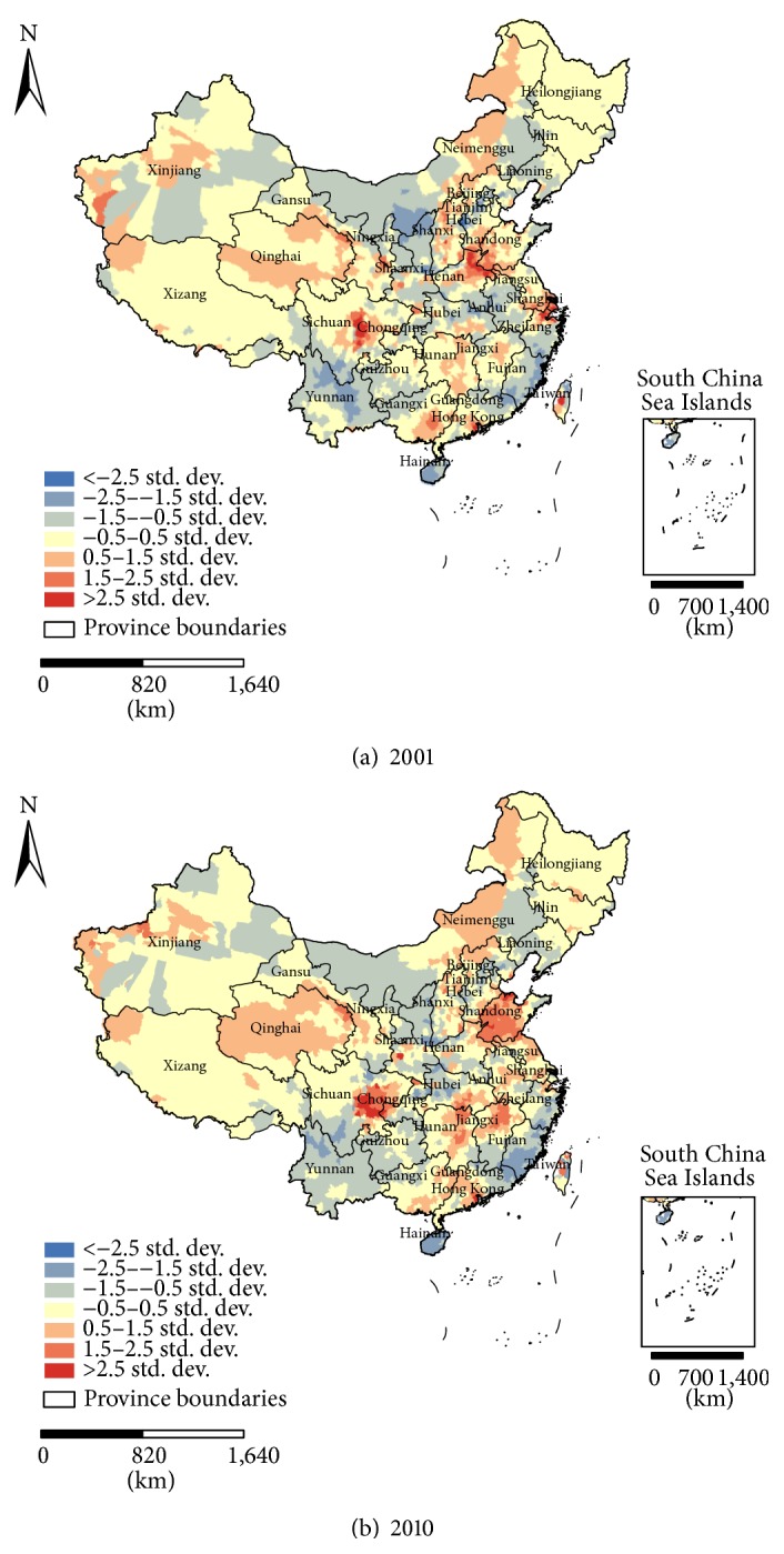
Maps of standardized residuals from the GWR model in China for (a) 2001 and (b) 2010.
The PM2.5, precipitation and temperature datasets used in this study were annual averaged values, which may introduce bias when evaluating the relationship between the datasets. There may be a strong seasonal variability in the PM2.5 concentration, and the PM2.5 concentrations are usually higher during the winter and summer than during the spring and fall [21]. In China, many studies also reported that PM2.5 concentrations vary in different seasons [41, 42]. In addition, the precipitation and temperature also exhibit a seasonal variability in China, and high precipitation and temperature are usually associated with the summer. Furthermore, Chen et al. [42] also found that the relationship between PM2.5 and meteorological parameters varied in different seasons in Beijing, China. Therefore, the correlation between PM2.5 concentrations, precipitation, and temperature would be affected by their seasonal variations. However, the lack of remote sensing datasets of PM2.5, precipitation, and temperature in different seasons is the primary obstacle to developing a model to study the relationship between the variables in different seasons. More studies that focus on seasonality are needed if detailed and high-resolution data can be obtained for future work.
5. Conclusions
In this study, the relationship between the PM2.5 concentrations and meteorological parameters and the spatial variance of the relationship in China during 2001–2010 were evaluated based on newly refined long-term data. The following main conclusions are attained.
-
(1)
The PM2.5 had a strong and stable correlation with the meteorological parameters, with a mean R value of 0.688 during 2001–2010 in China; thus, a negative correlation existed with the AAP and positive correlation existed with the AAT.
-
(2)
In general, the relationship between the PM2.5 and meteorological parameters varied over space. A strong negative correlation between the PM2.5 and AAP mainly appeared in the warm temperate semihumid region and the east-central areas of the northern subtropical humid region in 2001 and in the southeastern warm temperate semihumid region and the east-central areas of the northern subtropical humid region in 2010; regions of strong correlations were reduced in 2010 compared with 2001. A strong positive correlation between the PM2.5 and the AAT mainly existed in the mid-temperate semiarid region, the humid, semihumid, and semiarid areas of the warm temperate regions, and the central northern subtropical humid region in 2001 and in the mid-temperate semiarid region, the humid, semihumid, and semiarid areas of the warm temperate regions, and the central and northeastern areas of northern subtropical humid region in 2010; the regions of strong correlations increased in 2010 compared to 2001.
This paper advances the study of the relationship between PM2.5 and meteorological parameters for the purpose of epidemiological studies. However, the problem is complex and requires more attention in the future.
Acknowledgments
The study was supported by the Chinese Academy of Sciences (Grant no. KZZD-EW-08) and the High Resolution Earth Observation Systems of National Science and Technology Major Projects (Grant no. 05-Y30B02-9001-13/15).
Conflict of Interests
The authors declare that they have no conflict of interests regarding the publication of this paper.
Authors' Contribution
Gang Lin and Jingying Fu contributed equally to this work.
References
- 1.H.I.O. Committee. Health Effects of Outdoor Air Pollution in Developing Countries of Asia: A Literature Review. Boston, Mass, USA: Health Effects Institute; 2004. (Special Report No. 15). [Google Scholar]
- 2.Pope C. A., III, Burnett R. T., Thun M. J., et al. Lung cancer, cardiopulmonary mortality, and long-term exposure to fine particulate air pollution. Journal of the American Medical Association. 2002;287(9):1132–1141. doi: 10.1001/jama.287.9.1132. [DOI] [PMC free article] [PubMed] [Google Scholar]
- 3.Dominici F., Peng R. D., Bell M. L., et al. Fine particulate air pollution and hospital admission for cardiovascular and respiratory diseases. Journal of the American Medical Association. 2006;295(10):1127–1134. doi: 10.1001/jama.295.10.1127. [DOI] [PMC free article] [PubMed] [Google Scholar]
- 4.Pope C. A., III, Ezzati M., Dockery D. W. Fine-particulate air pollution and life expectancy in the United States. The New England Journal of Medicine. 2009;360(4):376–386. doi: 10.1056/NEJMsa0805646. [DOI] [PMC free article] [PubMed] [Google Scholar]
- 5.Harrison R. M., Yin J. Particulate matter in the atmosphere: which particle properties are important for its effects on health? Science of the Total Environment. 2000;249(1–3):85–101. doi: 10.1016/S0048-9697(99)00513-6. [DOI] [PubMed] [Google Scholar]
- 6.Gauderman W. J., Avol E., Gilliland F., et al. The effect of air pollution on lung development from 10 to 18 years of age. The New England Journal of Medicine. 2004;351(11):1057–1067. doi: 10.1056/NEJMoa040610. [DOI] [PubMed] [Google Scholar]
- 7.Zhao B., Wang P., Ma J. Z., Zhu S., Pozzer A., Li W. A high-resolution emission inventory of primary pollutants for the Huabei region, China. Atmospheric Chemistry and Physics. 2012;12(1):481–501. doi: 10.5194/acp-12-481-2012. [DOI] [Google Scholar]
- 8.Xin J. Y., Wang L. L., Wang Y. S., Li Z. Q., Wang P. C. Trends in aerosol optical properties over the Bohai Rim in Northeast China from 2004 to 2010. Atmospheric Environment. 2011;45(35):6317–6325. doi: 10.1016/j.atmosenv.2011.08.052. [DOI] [Google Scholar]
- 9.Hoff R. M., Christopher S. A. Remote sensing of particulate pollution from space: have we reached the promised land? Journal of the Air & Waste Management Association. 2009;59(6):645–675. doi: 10.3155/1047-3289.59.6.645. [DOI] [PubMed] [Google Scholar]
- 10.Martin R. V. Satellite remote sensing of surface air quality. Atmospheric Environment. 2008;42(34):7823–7843. doi: 10.1016/j.atmosenv.2008.07.018. [DOI] [Google Scholar]
- 11.van Donkelaar A., Martin R. V., Park R. J. Estimating ground—level PM2.5 using aerosol optical depth determined from satellite remote sensing. Journal of Geophysical Research: Atmospheres (1984–2012) 2006;111(21) [Google Scholar]
- 12.Chu D. A., Kaufman Y. J., Ichoku C., Remer L. A., Tanré D., Holben B. N. Validation of MODIS aerosol optical depth retrieval over land. Geophysical Research Letters. 2002;29(12):MOD2-1–MOD2-4. [Google Scholar]
- 13.Chu D. A. Analysis of the relationship between MODIS aerosol optical depth and PM2.5 in the summertime US. International Society for Optics and Photonics; August 2006; [DOI] [Google Scholar]
- 14.Engel-Cox J. A., Holloman C. H., Coutant B. W., Hoff R. M. Qualitative and quantitative evaluation of MODIS satellite sensor data for regional and urban scale air quality. Atmospheric Environment. 2004;38(16):2495–2509. doi: 10.1016/j.atmosenv.2004.01.039. [DOI] [Google Scholar]
- 15.Kumar N., Chu A., Foster A. An empirical relationship between PM2.5 and aerosol optical depth in Delhi Metropolitan. Atmospheric Environment. 2007;41(21):4492–4503. doi: 10.1016/j.atmosenv.2007.01.046. [DOI] [PMC free article] [PubMed] [Google Scholar]
- 16.Schäfer K., Harbusch A., Emeis S., Koepke P., Wiegner M. Correlation of aerosol mass near the ground with aerosol optical depth during two seasons in Munich. Atmospheric Environment. 2008;42(18):4036–4046. doi: 10.1016/j.atmosenv.2008.01.060. [DOI] [Google Scholar]
- 17.Hu Z. Spatial analysis of MODIS aerosol optical depth, PM2.5, and chronic coronary heart disease. International Journal of Health Geographics. 2009;8(1, article 27) doi: 10.1186/1476-072X-8-27. [DOI] [PMC free article] [PubMed] [Google Scholar]
- 18.Liu Y., Park R. J., Jacob D. J., Li Q., Kilaru V., Sarnat J. A. Mapping annual mean ground-level PM2.5 concentrations using multiangle imaging spectroradiometer aerosol optical thickness over the contiguous United States. Journal of Geophysical Research D: Atmospheres. 2004;109(22) doi: 10.1029/2004JD005025.D22206 [DOI] [Google Scholar]
- 19.Koelemeijer R. B. A., Homan C. D., Matthijsen J. Comparison of spatial and temporal variations of aerosol optical thickness and particulate matter over Europe. Atmospheric Environment. 2006;40(27):5304–5315. doi: 10.1016/j.atmosenv.2006.04.044. [DOI] [Google Scholar]
- 20.Schaap M., Apituley A., Timmermans R. M. A., Koelemeijer R. B. A., de Leeuw G. Exploring the relation between aerosol optical depth and PM2.5 at Cabauw, the Netherlands. Atmospheric Chemistry and Physics. 2009;9(3):909–925. doi: 10.5194/acp-9-909-2009. [DOI] [Google Scholar]
- 21.Liu Y., Sarnat J. A., Kilaru V., Jacob D. J., Koutrakis P. Estimating ground-level PM2.5 in the Eastern United States using satellite remote sensing. Environmental Science and Technology. 2005;39(9):3269–3278. doi: 10.1021/es049352m. [DOI] [PubMed] [Google Scholar]
- 22.Paciorek C. J., Liu Y., Moreno-Macias H., Kondragunta S. Spatiotemporal associations between GOES aerosol optical depth retrievals and ground-level PM2.5. Environmental Science and Technology. 2008;42(15):5800–5806. doi: 10.1021/es703181j. [DOI] [PubMed] [Google Scholar]
- 23.van Donkelaar A., Martin R. V., Brauer M., et al. Global estimates of ambient fine particulate matter concentrations from satellite-based aerosol optical depth: development and application. Environmental Health Perspectives. 2010;118(6):847–855. doi: 10.1289/ehp.0901623. [DOI] [PMC free article] [PubMed] [Google Scholar]
- 24.Zheng J., Yin Y., Li B. A new scheme for climate regionalization in China. Acta Geographica Sinica. 2010;65(1):3–13. [Google Scholar]
- 25.Lin G., Fu J., Jiang D., et al. Spatio-temporal variation of PM2.5 concentrations and their relationship with geographic and socioeconomic factors in China. International Journal of Environmental Research and Public Health. 2014;11(1):173–186. doi: 10.3390/ijerph110100173. [DOI] [PMC free article] [PubMed] [Google Scholar]
- 26.Li X. Characteristic of meteorological annual variety in Xi'an city and the relevant analysis of PM10 pollution characteristic (in Chinese with English Abstract) [M.S. thesis] Xi'an University of Architecture and Technology; 2003. [Google Scholar]
- 27.Ma S. A study on statistical characteristics and influenceing meteorlogical factors of PM 10 concentration in Yinchuan City duiing 2000–2012(in Chinese with English Abstract) [M.S. thesis] Lanzhou University; 2003. [Google Scholar]
- 28.Battelle Memorial Institute and Center for International Earth Science Information Network (CIESIN) Global Annual Average PM2.5 Grids from MODIS and MISR Aerosol Optical Depth (AOD) Palisades, NY, USA: NASA Socioeconomic Data and Applications Center (SEDAC); 2013. [Google Scholar]
- 29.World Health Organization; Regional Office for Europe. Air Quality Guidelines: Global Update 2005: Particulate Matter, Ozone, Nitrogen Dioxide, and Sulfur Dioxide. World Health Organization; 2006. [Google Scholar]
- 30.Ma J., Zhang W., Luo L., Xu Y. China Statistical Yearbook-2013. 2013. [Google Scholar]
- 31.Fotheringham A. S., Charlton M. E., Brunsdon C. Geographically weighted regression: a natural evolution of the expansion method for spatial data analysis. Environment and Planning A. 1998;30(11):1905–1927. doi: 10.1068/a301905. [DOI] [Google Scholar]
- 32.Zhang J. Research on the spatial variation of the urban housing land prices based on geographically weight regression model-a case study of Hangzhou [M.S. thesis] Zhejiang University; 2012. (in Chinese with English Abstact) [Google Scholar]
- 33.Fotheringham A. S., Brunsdon C., Charlton M. Geographically Weighted Regression: The Analysis of Spatially Varying Relationships. New York, NY, USA: John Wiley & Sons; 2002. [Google Scholar]
- 34.Hurvich C. M., Simonoff J. S., Tsai C. L. Smoothing parameter selection in nonparametric regression using an improved Akaike information criterion. Journal of the Royal Statistical Society. Series B. Statistical Methodology. 1998;60(2):271–293. doi: 10.1111/1467-9868.00125. [DOI] [Google Scholar]
- 35.Belsley D. A., Kuh E., Welsch R. E. Regression Diagnostic. John Wiley & Sons; 2005. Detecting and assessing collinearity; pp. 85–191. [Google Scholar]
- 36.Leung Y., Mei C.-L., Zhang W.-X. Statistical tests for spatial nonstationarity based on the geographically weighted regression model. Environment and Planning A. 2000;32(1):9–32. doi: 10.1068/a3162. [DOI] [Google Scholar]
- 37.Lü J. M., Ju J. H., Ren J. Z., Gan W. W. The influence of the Madden-Julian Oscillation activity anomalies on Yunnan's extreme drought of 2009-2010. Science China Earth Sciences. 2012;55(1):98–112. doi: 10.1007/s11430-011-4348-1. [DOI] [Google Scholar]
- 38.Yi H. Research on the characteristics of drought climate and the formation analysis for the extreme drought event from 2009 to 2012 in Southwest China [M.S. thesis] Lanzhou, China: Lanzhou University; 2013 (Chinese) [Google Scholar]
- 39.Hu X., Waller L. A., Al-Hamdan M. Z., et al. Estimating ground-level PM2.5 concentrations in the southeastern U.S. using geographically weighted regression. Environmental Research. 2013;121:1–10. doi: 10.1016/j.envres.2012.11.003. [DOI] [PubMed] [Google Scholar]
- 40.Tian J., Chen D. A semi-empirical model for predicting hourly ground-level fine particulate matter (PM2.5) concentration in southern Ontario from satellite remote sensing and ground-based meteorological measurements. Remote Sensing of Environment. 2010;114(2):221–229. doi: 10.1016/j.rse.2009.09.011. [DOI] [Google Scholar]
- 41.Shao L., Yang S., Shi Z. Study on the Physical, Chemical characteristics and Biological Activity of Particulate Matter in Urban Areas. Meteorological Press; 2006 (Chinese) [Google Scholar]
- 42.Chen Y., Cen K. S., Norra S., Schleicher N. Study on pollution characteristics of PM2.5 in the Aerosol, tracing and tracking atmospheric particulates in Beijing City. Geosciences. 2010;24(2):345–354. [Google Scholar]


