Chromosomal locus tracking with proper accounting of static and dynamic errors

Abstract

The mean-squared displacement (MSD) and velocity autocorrelation (VAC) of tracked single particles or molecules are ubiquitous metrics for extracting parameters that describe the object’s motion, but they are both corrupted by experimental errors that hinder the quantitative extraction of underlying parameters. For the simple case of pure Brownian motion, the effects of localization error due to photon statistics (“static error”) and motion blur due to finite exposure time (“dynamic error”) on the MSD and VAC are already routinely treated. However, particles moving through complex environments such as cells, nuclei, or polymers often exhibit anomalous diffusion, for which the effects of these errors are less often sufficiently treated. We present data from tracked chromosomal loci in yeast that demonstrate the necessity of properly accounting for both static and dynamic error in the context of an anomalous diffusion that is consistent with a fractional Brownian motion (FBM). We compare these data to analytical forms of the expected values of the MSD and VAC for a general FBM in the presence of these errors.

I. INTRODUCTION

Camera-based particle tracking has been an important tool for the study of biophysical systems and other condensed-matter environments at the single-molecule and single-particle level for decades. A particle to be tracked is most often labeled with a fluorescent or scattering marker and imaged with a wide-field microscope over time. The particle’s spatial trajectory is thus recorded and further analysis can reveal properties of both the tracer and the surrounding medium. In biology this has been applied to the study of molecular motors [1], motion in membranes [2–5], and motion throughout the three-dimensional (3D) volume of the cytoplasm [6–9] or nucleoplasm [10–12], to name a few instances.

The most ubiquitous statistical measure used to analyze single-particle tracking data is the mean-squared displacement (MSD). Arguably the next most important metric is the velocity autocorrelation (VAC) function, and more sophisticated measures such as those based on maximum likelihood [13] or covariance-based estimation [14] are closely related to the VAC. In a real experiment, one cannot directly measure the true MSD or VAC but rather must estimate them, either by calculating time averages or ensemble averages, or combining the two if the underlying process is ergodic. In addition to being susceptible to sampling statistics from finite track lengths and numbers [15,16], the estimated MSD and VAC also depend on two major sources of error: (1) zero-mean Gaussian localization error due to photon statistics (referred to as “static error”), and (2) motion blur due to finite exposure time (referred to as “dynamic error”). Static and dynamic errors are always present to some degree, and proper care must be taken to account for them when analyzing any MSD or VAC. The equations that take these errors into account are well known for the special case of pure Brownian motion, but less so for the more experimentally relevant case of anomalous diffusion. We present derived equations that take both of these errors into account for both the MSD and VAC of an anomalously diffusing object obeying a fractional Brownian motion (FBM). In fact, the equation for such an MSD was derived a decade ago by Savin and Doyle [17], yet the particle tracking community has not widely used it when appropriate. Biologically oriented studies often neglect both sources of error, while more quantitative studies sometimes consider the static error but not the dynamic error. We show that the dynamic error must also be considered for anomalous diffusion, especially when the static error has been carefully removed or mitigated as the leading literature advises [18–20]. The expression presented here for the VAC in the presence of errors represents a generalization of the corresponding MSD. We demonstrate the utility of these expressions by application to experimental data of tracked chromosomal loci in budding yeast nuclei, as well as to simulated data. Importantly, when the same object is tracked in two emission color channels with different detected photon numbers, we show directly that the correct parameters of motion can be extracted from either measurement when the proper expressions are used.

II. RESULTS AND DISCUSSION

A. Mean-squared displacement (MSD)

For the simplest case of pure Brownian motion, the MSD, denoted here by the function M(·), scales linearly with time lag; i.e., M(n) = 2Dnt_E, where D is the diffusion coefficient, t_E is the exposure time of the camera acquisition, and n is the number of frames spanning the lag. Throughout this paper we also refer to the time lag as δ = nt_E, and so the MSD in this case is M(δ) = 2Dδ. This expression is valid for tracking in one dimension (1D), though extension to 3D is trivially achieved by adding the MSDs of three 1D processes together. We assume here and throughout this paper that the sample is illuminated continuously and that there is no time elapsed between recorded frames. This situation is common in most experimental situations, though extension to stroboscopic or time-lapse imaging is straightforward, as shown previously for the case of pure Brownian motion [13,21,22]. The effect of static and dynamic errors on the expected value of the estimated 1D MSD for the special case of pure Brownian motion is to produce a constant offset of the linear dependence according to Eq. (1) [13,17,21,22]:

$$E[\widehat{M}(n)]=2{\mathit{Dnt}}_E+2{\sigma }^2-\frac{2}{3}{Dt}_E,$$ (1)

where the E[·] refers to the expectation value and the hat denotes the estimated quantity. We make a point to indicate the expected value explicitly, as real data will show fluctuations about this value due to the aforementioned finite sampling statistics, which we discuss in more depth below. The form of Eq. (1) has been known for some time, though recent papers have pointed out that the σ that appears in Eq. (1) is not the same as the localization error of an immobile particle σ₀, but instead includes an additional correction due to the spreading of photons over a greater area of the detector for a moving particle [22,23]. We discuss this in more detail in the next section. While Eq. (1) holds for a particle undergoing pure Brownian motion, it does not apply for the more general case of anomalous diffusion, despite the importance of anomalous diffusion in biology.

Anomalous diffusion refers to motion with an MSD of the form M(n) = 2D^*(nt_E)^α, where D^* is an effective diffusion coefficient and α∈(0,2]. Motion with α > 1 is referred to as “superdiffusive,” while α < 1 specifies motion which is “subdiffusive.” Subdiffusion is often observed in biology and other complex systems, and a number of underlying models have been invoked to explain various subdiffusive phenomena, including most commonly obstructed diffusion [24], continuous time random walk [25], and fractional Brownian motion (FBM) [26]. While some or all of these models and others can be consistent with a given MSD scaling, a number of tests have been developed to distinguish among them [16,27–35]. For a thorough review see [36].

Certain previous studies have addressed some of the effects of static or dynamic errors on the MSD of subdiffusive processes. Static error is known to cause the log-log MSD curve (which otherwise has constant slope α) to bend upward at early times, causing potential underestimation of α [18–20]. It is easy to show that the static error presents itself as an additive offset of 2σ² as in the pure Brownian case, and so the static error is sometimes accounted for by assuming an MSD of the form

$$E[\widehat{M}(n)]=2D^{\ast }{({nt}_E)}^{\alpha }+2{\sigma }^2.$$ (2)

Despite this fact, it is still very common in the literature to either ignore the offset due to this error or dismiss it as irrelevant based on a somewhat qualitative assessment. When more thoroughly addressed, an experimenter typically either fits the computed MSD with Eq. (2) directly by allowing for a positive constant offset, or they estimate σ independently and subtract the appropriate term from the computed MSD. However, there are some cases in which these treatments are insufficient as the dynamic error is also significant.

Our experimental application to chromosomal tracking in yeast provides such a case. We tracked copies of a single chromosomal locus (POA1) just downstream of the GAL locus of genes (GAL 7, 10, and 1) [11,37] in live G1 phase Saccharomyces cerevisiae cells using the LacO/LacI-GFP (green fluorescent protein) labeling system [38] in a wide-field fluorescence microscope. This strain was previously used as a control for a study on velocity cross-correlations of distinct loci on yeast chromosomes [39]. In that study we were surprised to find that α was in the range 0.6–0.75 for all strains we measured, in contrast to the previously reported value for GAL in yeast of ~0.45 [11]. We determined that the most likely explanation for this discrepancy was the effects of localization errors; here we explore the effects of static and dynamic errors in the control strain in much greater detail. We collected data from 120 tracks in as many cells, consisting of, on average, 338 ± 94 frames (± means standard deviation) taken with t_E = 100 ms. Data were acquired using the double-helix point spread function (DHPSF) microscope, which allows for 3D wide-field tracking by encoding the z position into the angle made between two closely spaced lobes of light [40,41] and a reference line. Three-dimensional positions were extracted via a least-squares fit to the sum of two 2D-Gaussian functions. Additional details regarding cell preparation, microscopy, and image analysis are given in [39]. A 2D projection from an example track is shown in the inset of Fig. 1(a).

FIG. 1.

(Color online) MSD for chromosomal loci in yeast. All error bars are S.E.M. from 100 bootstrapped samples of the ensemble. Each panel depicts data from the green channel MSD (green or light gray), red channel MSD (red or darker gray), and “cross-MSD” (black). (a) Dots are data points computed from experimental data. Solid lines are fits to Eq. (8). (Inset) Example image of 2D-projected locus track in white light image of a yeast cell. This example is from a diploid, but all cells analyzed here were haploids. Scale bar: 1 μm. (b) Naïve estimates of α from fitting to a straight line in log-log space. Each point corresponds to fitting all points from n = 1 through the marked time point. (c) Estimates of α taking only static error into account. Only estimates corresponding to five points or more are shown since the nonlinearity requires several points to be reliably fit (see Fig. S11 [46] and discussion in main text). (d) Estimates of α taking both static and dynamic error into account; plotted points start at n = 5 for the same reason as in (c).

Images were recorded on a microscope consisting of two color channels (green and red) split by a dichroic mirror, with DHPSF-encoding transmissive phase masks located at the Fourier plane in both paths [42]. Because the labeling system typically resulted in ~20–30 GFP labels bound to the locus at a time, the combination of the sum of many emitters and the red-extending tail of the GFP emission spectrum allowed for tracking of the same particle simultaneously in both color channels, albeit with significantly disparate localization errors. We stress that there is no difference between the particles’ motion in the red and green channels since we simultaneously tracked the same 120 particles in each channel. Yet the disparate localization errors cause the computed ensemble-mean time-averaged MSDs to appear very differently [Fig. 1(a)], only beginning to coincide at large n. Because the particles appeared significantly dimmer in the red channel, the static error was larger in this channel and thus the MSD curves upward with a significantly shallower slope in log-log space. Of course the green channel must also suffer from nonzero static error, and yet the green MSD appears to be relatively constant in its slope. Does this mean that the static error is small enough to be ignored in the green channel? On the contrary, we argue that the apparently constant slope is a lucky accident since our experimental configuration allows us to effectively remove the static error in the following way: because the random photons hitting the detector in either channel are independent of one another, the random static errors in each channel are also independent of one another. Thus we can compute the MSD in a third way by multiplying each displacement recorded in the red channel by the simultaneously determined displacement in the green channel and then averaging. The result is the “cross-MSD” shown in black in Fig. 1(a). With the static error now effectively removed (only leaving a small residual error from the registration of the two channels [42,43]) we see that the MSD curve does not assume a perfectly straight line as Eq. (2) would suggest. Instead we see that the cross-MSD bends downward at early times—a consequence of the still-present dynamic error.

An accurate model for the MSD should produce estimates of α which coincide for all three computed MSDs. The most naïve estimation is shown in Fig. 1(b). Here we fit each MSD in log-log space to a straight line, as one would expect in the absence of errors. We include a variable number of points in the fit, and show the estimates over a range of time scales. Unsurprisingly, the red (top, gray), green (middle, light gray), and black plots in Fig. 1(b) do not coincide at all, as the red estimates starts from far below around 0.3, the black starts from significantly above near 1.0, and the green remains in the range 0.6–0.8, sloping slightly downward at early times. If we instead fit the log-log MSDs by allowing for a positive offset from static error according to Eq. (2) we produce the estimates plotted in Fig. 1(c) . The red estimation changes dramatically as we would expect. While the green and red estimates now coincide after ~2 s, there is still a small but significant discrepancy at earlier times. Most notably, the black estimates from the cross-MSD are still significantly inflated relative to the others. It is clear that Eq. (2) is insufficient to make our experimental results self-consistent. Thus we seek an extension of Eq. (2) that properly incorporates the effects of dynamic error for the case of anomalous diffusion.

The manifestation of dynamic error in the MSD of an anomalous diffusion is more elusive in the literature than that of static error. It has been described previously in the specific contexts of “hop” and confined diffusion [3,44,45]. We instead sought a generalization of the pure Brownian motion case given in Eq. (1) valid for any FBM with arbitrary α. The full derivation is given in the Supplemental Material [46] and here we sketch the derivation and present the result. As it turns out, the resulting equation for the MSD was derived a different way and stated a decade ago in [17], but application to appropriate cases in the literature is lacking. The full, overlooked equation is required to help resolve standing discrepancies in the tracking literature and so we here restate the result and apply it to tracked chromosomal loci to demonstrate its importance.

FBM is the self-similar process that has Gaussian, stationary increments [26]. Denoting the position of a particle undergoing FBM at time t as x(t), such a particle exhibits a characteristic autocovariance function between positions at two times [47]:

$$E[x(t_1)x(t_2)]=D^{\ast }\left(t_1^{\alpha }+t_2^{\alpha }-{\mid t_1-t_2\mid }^{\alpha }\right).$$ (3)

One can easily show that Eq. (3) implies that pairs of increments exhibit negative correlation when α < 1 (resulting in subdiffusion), no correlation when α = 1 (resulting in pure Brownian motion), positive correlation when α > 1 (resulting in superdiffusion), and perfect correlation when α = 2 (resulting in constant-velocity motion). Thus, pure Brownian motion and ballistic or directed motion are special cases of FBM. We chose to work specifically within the framework of FBM since our chromosomal loci demonstrated the characteristic Gaussian increments and velocity correlations (vide infra) consistent with this motion [39]. Also, FBM and the closely related fractional Langevin motion have been implicated in a number of other previous instances of particles and biopolymers traversing the cellular cytoplasm and nucleoplasm, including mRNA and DNA loci in E. coli [28,35,39,48], lipid granules in fission yeast (at least at long times [49]), and telomeres in mammalian cells [12,31].

Using Eq. (3) and an extension of the formalism used by Michalet [22] to derive the variance of position estimation of a Brownian diffuser, we derived the FBM analog of Eq. (1). Briefly, we assume that a particle moving in 1D undergoes FBM with specified D^* and α, and that within an imaging frame the particle emits a random number of photons p ~ Poisson(p̄). The ith photon during the kth frame is recorded at a position that is the sum of the position of the particle at the time of emission, $x_i^{(k)}$, and a random variable ${\xi }_i^{(k)}$, with $E({\xi }_i^{(k)})=0$ and $var({\xi }_i^{(k)})=s_0^2$, that accounts for static error. Here s₀ is set by the width of the point spread function (PSF) of the microscope. The estimated position of the particle during the kth frame, ${\widehat{x}}_k={\sum }_{i=1}^p[x_i^{(k)}+{\xi }_i^{(k)}]/p$, is the centroid position of the recorded photons during that frame. While this formalism does not explicitly account for background, pixelation of the image, alternative position estimators, or extension to more spatial dimensions, we show below that simple modifications to the final result are sufficient to do so.

The derivation then proceeds by finding an expression for E[M̂(n)] = E[(x̂_k+n − x̂_k)²]. Naturally, the final result will not depend on k since FBM is a stationary increment process [12,26,31,50]. As shown in the Supplemental Material [46], this approach yields the analytical expression

$$E[\widehat{M}(\delta )]=\frac{2D^{\ast }}{(\alpha +2)(\alpha +1)t_E^2}\times [{(\delta +t_E)}^{\alpha +2}+{(\delta -t_E)}^{\alpha +2}-2{\delta }^{\alpha +2}]-\frac{4D^{\ast }{t}_E^{\alpha }}{(\alpha +2)(\alpha +1)}+\frac{2}{\overline{p}}\left[s_0^2+\frac{2D^{\ast }{t}_E^{\alpha }}{(\alpha +2)(\alpha +1)}\right].$$ (4)

This form is consistent with Eq. (30) presented in [17], which in fact holds for any motion obeying the appropriate power-law MSD (i.e., not just FBM).

Examination of Eq. (4) gives rise to a number of interesting observations. For one, an algebraic check confirms the key limit: for D = D^* and α = 1 (thus specifying pure Brownian motion) we indeed recover Eq. (1) if we allow the equivalence in Eq. (5):

$${\sigma }^2={\sigma }_0^2+\frac{{Dt}_E}{3\overline{p}}$$ (5)

where ${\sigma }_0^2=s_0^2/\overline{p}$ is the true static error of an unmoving particle. The term that is proportional to D in Eq. (5) results from the fact that the effective PSF of a moving object is effectively larger than that of a stationary one. This term was found previously via a different derivation [23] and typically only results in a small inflation of σ. This term settles a standing discrepancy in the literature in that a similar expression was also previously reported in [22], but mistakenly without the factor of 3 in the denominator.

Inspection of Eq. (4) shows that the generalized version of the static error term given by Eq. (5) is now given by Eq. (6):

$${\sigma }^2={\sigma }_0^2+\frac{2D^{\ast }{t}_E^{\alpha }}{(\alpha +2)(\alpha +1)\overline{p}}.$$ (6)

We can thus state the relative increase of the static localization error due to the particle motion as

$$\frac{\sigma }{{\sigma }_0}=\sqrt{1+\frac{2D^{\ast }{t}_E^{\alpha }}{(\alpha +1)(\alpha +2)s_0^2}}.$$ (7)

Compared with the α = 1 case, a significant increase of σ/σ₀ can be expected for lower α for a given D^* and t_E. This is shown in Fig. S1 [46] for various parameters. As an example, for D^* = 0.2 μm²/s^α, t_E = 10 ms, s₀ = 0.214 μm, and α = 1, Eq. (7) yields a ratio of 1.007, i.e., an increase of less than 1%. However, for the same parameters except α = 0.4, the increase is ~19%, and so is significant. Thus, when one performs an independent measure of σ₀ in order to subtract the positive offset from the MSD, the entire positive offset may not be fully removed, particularly when α is low. In any case we can rewrite Eq. (4) as

$$E[\widehat{M}(n)]=\frac{2D^{\ast }{t}_E^{\alpha }}{(\alpha +2)(\alpha +1)}[{(n+1)}^{\alpha +2}+{(n-1)}^{\alpha +2}-2n^{\alpha +2}]-\frac{4D^{\ast }{t}_E^{\alpha }}{(\alpha +2)(\alpha +1)}+2{\sigma }^2,$$ (8)

where we have also factored out $t_E^{\alpha +2}$ from the bracketed portion of the first term in order to write the expression in terms of n rather than δ. By fitting to Eq. (8) and allowing σ to be a positive free parameter we automatically take into account any dilation of the form in Eq. (6). This approach also automatically accounts for the fact that the exact form of Eq. (6) depends on the choice of estimator (see below).

The effects of the dynamic error in the pure Brownian case [Eq. (1)] are captured in the term −2Dt_E/3. The generalized version of this term that appears in Eq. (8) is $-4D^{\ast }{t}_E^{\alpha }/[(\alpha +2)(\alpha +1)]$. In Eq. (8) there exists still another consequence of the dynamic error in that the first bracketed term contains powers of n beyond just n^α. At first glance this seems somewhat peculiar, but expansion of the relevant term into an infinite sum gives further insight:

$$\frac{[{(n+1)}^{\alpha +2}+{(n-1)}^{\alpha +2}-2n^{\alpha +2}]}{(\alpha +2)(\alpha +1)}=\sum _{k=0}^{\infty }\left(\begin{array}{c}\alpha \\ k\end{array}\right)n^{\alpha -k}\left[\frac{1+{(-1)}^k}{(k+2)(k+1)}\right].$$ (9)

Here the factor $\left(\begin{array}{c}\alpha \\ k\end{array}\right)$ is a generalized binomial coefficient and is formally defined via a ratio of gamma functions:

$$\left(\begin{array}{c}\alpha \\ k\end{array}\right)=\frac{\mathrm{\Gamma }(\alpha +1)}{\mathrm{\Gamma }(k+1)\mathrm{\Gamma }(\alpha -k+1)}=\frac{\mathrm{\Gamma }(\alpha +1)}{k!\mathrm{\Gamma }(\alpha -k+1)},$$ (10)

for integer k and possible noninteger α.

Evidently the leading nonzero term in Eq. (9) is actually still n^α. We expand the infinite sum to include only the first few nonzero terms:

$$\frac{[{(n+1)}^{\alpha +2}+{(n-1)}^{\alpha +2}-2n^{\alpha +2}]}{(\alpha +2)(\alpha +1)}\approx n^{\alpha }+\frac{\alpha (\alpha -1)}{12}{n}^{\alpha -2}+\frac{\alpha (\alpha -1)(\alpha -2)(\alpha -3)}{360}{n}^{\alpha -4}.$$ (11)

The terms beyond n^α decay rapidly. In some special cases, however, they can be somewhat significant. By inspection, the extra terms are most significant when n = 1, i.e., at the first point of the MSD. For simplicity consider this case when σ = 0 (or more realistically when σ has been measured and the corresponding offset has been removed). Figure S2 [46] shows the importance of including the extra terms as a function of α at this first point of the MSD relative to the case of just including the negative constant offset. Note that when α = 1 Eq. (9) evaluates exactly to the linear term n—the cubic, square, and constant terms exactly cancel one another. When the displacements are uncorrelated the additional power terms disappear, and so equivalently the appearance of these terms is a direct consequence of the presence of correlations in the motion. For subdiffusive α, the effect is small, as it only affects the MSD at this point by ~5% – 10% below α = 0.6. For superdiffusive α, however, the effect is indeed significant as it approaches 20% as α → 2, so while the extra terms in Eq. (9) are mathematically interesting, they likely do not have a very significant effect on fitting of the MSD except in some superdiffusive cases. We will show in the next section, however, that these terms can indeed make a difference when considering the VAC for subdiffusive cases.

With the theory paved we now return to our chromosomal locus tracking data. Fitting each of the three MSD curves in Fig. 1(a) using Eq. (8) and allowing three free parameters (α, D^*, and σ) gives the results shown in Fig. 1(d). Clearly now the three cases coincide quite closely with one another on all time spans considered. We note that there might be some relatively small, nonconstant temporal dependence of the estimated α parameter. This may reflect a real but modest amount of nonstationarity over the time scale considered. This may also be a manifestation of heterogeneity within the ensemble, as this appears consistent with the effect reported in [19]. To give an indication of the heterogeneity within our sample, Fig. S3(a) [46] shows the individual time-averaged cross-MSDs of each of the 120 experimentally obtained trajectories. To the same end, Fig. S3(b) [46] gives the histogram of estimated α̂_cross values as determined from the individual trajectories. The mean of the distribution is 0.74 and the standard deviation is 0.26. The width of the distribution of estimated α is indeed comparable to those explored in [19]. We note, however, that this finite width of the distribution is a function of the finite track lengths, static error, and dynamic error, in addition to the true underlying heterogeneity. A thorough treatment of heterogeneity in the presence of these factors is saved for future work.

Estimating α from the ensemble mean of the MSDs gives the same value as taking the mean of the individual estimates. In particular, the results of fitting the full 10 s of the ensemble-mean curves show remarkable agreement with the center of the distribution of individual estimates and with one another: α̂_green = 0.74 ± 0.03, α̂_red = 0.74 ± 0.04, and α̂_cross = 0.74 ± 0.03 (error is standard error of the mean [S. E. M.] as determined from 100 bootstrapped samples of the individual tracks). To the precision of two significant figures, all three fits gave D̂^* = (1.7 ± 0.1) × 10⁻³ μm²/s^α. The estimated 3D localization precisions for the three cases are σ̂_green = 26 ± 2 nm, σ̂_red = 59 ± 2 nm, and σ̂_cross = 13 ± 2 nm. Note that the 3D localization precision is related to the x, y, and z precisions via $\sigma =\sqrt{{\sigma }_x^2+{\sigma }_y^2+{\sigma }_z^2}$. The residual precision for the cross-MSD case is on the order of what we expect with our registration method [39,42]. Thus we directly demonstrate that experimental measurements with different degrees of error produce the same estimates for the underlying parameters of motion when the proper expression is used.

To further compare Eq. (8) to data over a range of motion and imaging parameters, we produced simulated FBM tracks in 1D, 2D, and 3D using the method of circulant embedding, with custom MATLAB code building upon the code provided in [51]. Tracks were simulated with t_E = 10 ms and various mean photon numbers per frame p̄. We generated the position of each recorded photon by adding the position of the particle at the (random) time of detection to a random number with PDF proportional to a simulated PSF. Photon positions within each frame were then grouped to produce position estimates. In 1D we estimated the positions via a simple centroid estimator such that Eq. (6) applies exactly as written. Figure S4 [46] shows the time-ensemble-averaged MSDs for this 1D simulated data with parameters α ∈ {0.2, 0.4, 0.6, 0.8, 1.0, 2.0}, D^* ∈ {10⁻³, 10⁻², 10⁻¹, 10⁰, 10¹} μm²/s^α, and p̄ ∈ {50, 500, 1500}. Figure S4 [46] reflects results from 100 tracks each consisting of 100 frames; the plotted points represent the ensemble mean of the time-averaged MSDs. We see excellent agreement between our simulations and the theoretical prediction in all cases, including those in which the errorless prediction either grossly over- or underestimates the curve. While the cases in which static error dominates can be matched by Eq. (2), the dynamic error must also be accounted for in order to match in other cases.

We compared these results to 2D simulations by producing two independent FBMs for x and y for each track via the method described above; independence between the x and y increments provides a sufficient but not necessary way to produce the relevant MSD statistics. Again we simulated 100 tracks each consisting of 100 frames. In each frame, photons (p̄ = 500) were binned into pixels of width a = 160 nm. A Poisson-distributed background with specified mean b was added to each pixel before fitting the resulting image with a 2D Gaussian function in order to estimate particle position. In each frame the estimated position was constrained to a region of interest (ROI) around the true position of the particle. In a real experiment this would correspond to cold starting the fitting near an obvious localization, e.g., by hand as in our chromosomal tracking experiments. The ROI then follows the particle by resetting each frame centered on the localization from the previous frame. Example simulated images are shown in Fig. 2(a) for α = 0.6, b = 0, and D^* ∈ {10⁻³, 10⁻², 10⁻¹, 10⁰, 10¹} μm²/s^α. Note that the effective size of the PSF increases with increasing D^*, though this only becomes noticeable when the increase is sufficiently larger than the diffraction limit. In fact, we can quantify this PSF broadening by multiplying s₀ by the right-hand side of Eq. (7) to give the dilated PSF width s. To model σ we then substituted this expression for s into a known expression for 2D localization error which takes background and pixelation into account. Such a model was proposed by Thompson et al. [52] and later made more accurate [53]:

$${\sigma }^2=\frac{16(s^2+a^2/12)}{9\overline{p}}+\frac{8\pi b{(s^2+a^2/12)}^2}{a^2{\overline{p}}^2}.$$ (12)

FIG. 2.

(Color online) (a) Example simulated images of particle diffusing within a single frame with α = 0.6, b = 0, and t_E = 10 ms. From left to right D^* is 10⁻³, 10⁻², 10⁻¹, 10⁰, and 10¹. Pixel size = 160 nm. (b) Resulting MSDs from 2D simulation of FBM for various α (top to bottom rows: α = 0.2, 0.4, 0.6) and b (left to right columns b = 0, 50, 100), with p̄ = 500 and (from bottom to top in each panel:) D⁻ = 10⁻³ (blue), 10⁻² (cyan), 10⁻¹ (green), 10⁰ (yellow), and 10¹ (red) μm²/s^α. Dots are simulated data, solid lines are theoretical predictions, and dashed lines are the predictions in the absence of errors.

This treatment of σ is analogous to that done in [23] for the case of pure Brownian motion. Note also that we must multiply the rest of Eq. (8) by a factor of 2 since the simulation at hand was done in 2D. The dots in Fig. 2(b) are compared to the solid lines generated by Eq. (8), while the dashed lines are the straight lines of slope α expected in the absence of errors. Additional data for α ∈ {0.4, 0.8, 2.0} are shown in Fig. S5 [46]. We omit the case of α = 0.2, D^* = 10 because in particular when b > 0, the images for this extreme subdiffusive motion would be unusable anyway since the signal is unidentifiable amid the noise (see Fig. S5, for example). Figure 2(b) clearly shows that we can accurately match the estimated MSD in 2D over a range of conditions, with pixelation and background, and using the more common Gaussian position estimator.

Finally, to compare Eq. (8) to 3D data over a range of parameters we extended our FBM simulations using a simulated DHPSF (Figs. S7 and S8 [46]). As in our experimental demonstration, we fit each simulated image to a sum of two 2D-Gaussian functions in order to estimate positions. Though we do not have a closed-form expression for σ in this case, with knowledge of the underlying true simulated motion we could compute it directly for the sake of comparison to Eq. (8).

Admittedly, the chosen track length and number of tracks considered in our simulations are somewhat arbitrary. As mentioned in the Introduction and known previously [15,16], these sources of finite statistics also cause errors in the computed MSD. For this reason we stress that Eq. (8) only represents the expected value (i.e., mean) of the MSD of an ensemble of finite-length trajectories. The full distribution will have a finite width that depends on track length. This fact is not a revelation unique to Eq. (8) or FBM. Indeed, fitting an individual pure Brownian track with Eq. (1) should be treated with similar care. Previous work has painstakingly detailed how many points should be ideally fit for a pure Brownian track of a given length, exposure time, and localization error [22], and derived the higher moments of the distribution of the estimated MSD under such circumstances. We reserve the derivation of the full distribution of the MSD of FBM for future work, as it becomes immediately much more involved to even derive the next moment of the distribution.

To partially explore the effects of finite track length, we shortened and reanalyzed the MSDs of the 2D simulated tracks described above. Figures S9 and S10 [46] show the full ensemble of 100 time-averaged MSDs, along with the mean of the ensemble compared to the curve expected from Eq. (8), for trajectory lengths of 25, 50, and 100 frames. These depict the particular case of t_E = 10 ms, D^* = 0.1 μm²/s^α, p̄ = 500, and b = 50; obviously this is only a slice within a massive parameter space. Figure S9 plots the data in linear space and Fig. S10 [46] in log-log space. While experimental constraints such as finite depth of focus or fluorophore bleaching can realistically limit trajectory lengths, it should always be possible to record a sufficiently high number of tracks, and so we did not explore the effects of the latter here further. By inspection, the ensemble mean in each case closely follows Eq. (8) except for a fraction of points at the largest lags, since there are fewer data to average at these lags. To be more to the point, we assessed the effects of shortened trajectory length by fitting variable numbers of points of the MSD to Eq. (8) for these simulated data. The results are shown in Fig. S11 and point to a very heuristically determined rule of thumb that fitting the first third of the points available gives reasonable accuracy and precision (<~0.1). Fitting too many points overvalues poorly averaged points. Fitting too few points makes it more difficult to detect nonlinear behavior since the limiting case of two points will always be consistent with α = 1 and some offset.

As mentioned, the effectiveness of this rule of thumb clearly will depend on the parameters of motion and imaging. Thus we fit the first third of the MSD for various D^* and b values and enumerated the resulting bias and error on estimated α. Figure S12 [46] shows the results from fitting to Eq. (8) with free parameters α, D^*, and σ. Estimation errors are still understandably best (<0.1) for the longest trajectory lengths, and for the highest ratios of D^*/σ. Figure S13 shows comparable errors when σ is measured and 2σ² is subtracted from the MSD before fitting with only two free parameters.

B. Velocity autocorrelation (VAC)

Next to the MSD, the VAC is perhaps the second-most common statistical metric employed in analyzing single-particle tracking data. In an experiment one can only compute the mean velocity between recorded frames according to (in 1D)

$${\widehat{v}}_k^{(n)}=\frac{{\widehat{x}}_{k+n}-{\widehat{x}}_k}{{nt}_E}.$$ (13)

Thus the expected value of the measured VAC in one dimension is defined as

$$E[{\widehat{C}}_v^{(n)}(m)]=\frac{E[({\widehat{x}}_{k+n}-{\widehat{x}}_k)({\widehat{x}}_{k+n+m}-{\widehat{x}}_{k+m})]}{{({nt}_E)}^2}.$$ (14)

Note the presence of two time indices n and m, or equivalently, two time variables δ = nt_E (time scale for defining velocity) and τ = mt_E (lag in VAC). Again, for a stationary increment process such as FBM the expectation does not depend on the index k. Note also that when m = 0 the VAC is proportional to the MSD:

$$E[{\widehat{C}}_v^{(n)}(m=0)]=\frac{E[\widehat{M}(n)]}{{({nt}_E)}^2}.$$ (15)

Hence the ensuing expression for the VAC of a particle undergoing FBM in the presence of both static and dynamic errors is a generalization of the previously described MSD.

It is straightforward to show that the defining covariance function of FBM in Eq. (3) implies the following VAC in the absence of errors:

$$C_v^{(n)}(m)=\frac{D^{\ast }{t}_E^{\alpha }}{{({nt}_E)}^2}[{(n+m)}^{\alpha }-2m^{\alpha }+{\mid n-m\mid }^{\alpha }].$$ (16)

For m ≥ n, this function is negative for α < 1, positive for α>1, and zero when α = 1. The characteristic negative signature is a key tool in distinguishing FBM from other modes of subdiffusion [ [28,54,55]. Most often the computed VAC is scaled by C_v⁽ⁿ⁾(m = 0) so that values at various n can be directly compared. For FBM the scaled VAC is

$$\frac{C_v^{(n)}(m)}{C_v^{(n)}(m=0)}=\frac{1}{2}\left[{\left(1+\frac{m}{n}\right)}^{\alpha }-2{\left(\frac{m}{n}\right)}^{\alpha }+{\left|1-\frac{m}{n}\right|}^{\alpha }\right].$$ (17)

The scaled VACs computed from our chromosomal loci data are plotted in Fig. 3, as determined in the green [Figs. 3(a) and 3(d)] and red [Figs. 3(b) and 3(e)] channels. The cross-correlation between the two channels is shown in Figs. 3(c) and 3(f). The bottom row of Fig. 3 shows a closer view of the first 2-s window depicted in the top row. The plotted values are the averages of the scaled VACs in x, y, and z. We plot and color code the VAC as computed for all n between 1 and 100. In all three cases we see negative values at each n. At sufficiently large n the minima appear to become more-or-less constant, as we would expect from Eq. (17) for all n. We fit each VAC (i.e., each colored curve in each panel) to Eq. (17) to again produce naïve estimates of α. These results are shown in Fig. 4(a). None of the cases agree well at early times, with the cross-correlation at higher α than in the green channel, and the red channel suggesting far lower α. At longer times the cross-correlation and green channel agree but the red estimates do not quite reach the others. Much as in the MSD case, our goal is to extend Eq. (16) to properly account for static and dynamic errors such that estimates of α coincide for the three cases.

FIG. 3.

(Color online) Computed scaled VACs across various time scales for chromosomal locus data from the green channel [(a) and (d)], the red channel [(b) and (e)], and the cross-correlated data [(c) and (f)]). Bottom row depicts the same curves from the first 2 s as in the top row, zoomed in and with a different color scale. The color scales for the top and bottom rows are shown on the right. For reference in gray scale version, larger δ corresponds to a curve with negative peak further to the right.

FIG. 4.

(Color online) Analysis of VACs from chromosomal loci data. All error bars are S.E.M. from 100 bootstrapped samples of the ensemble. Each panel depicts data from the green channel VAC (green or light gray), red channel VAC (red or darker gray), and cross-correlation (black). (a) Estimates of α resulting from naïve fits of the VACs without accounting for static or dynamic error. (b) Estimates of α resulting from taking static error into account, but not dynamic error. (c) Estimates of α taking both static and dynamic error into account. (d) Example computed and fit VACs for n = 1. Dots with error bars are computed from data; solid lines are fits taking static and dynamic error into account.

The effects of static error on the VAC have been characterized previously [28]. Namely, this error results in constant offsets at two particular points:

$$E[{\widehat{C}}_v^{(n)}(m)]=\frac{D^{\ast }{t}_E^{\alpha }}{{({nt}_E)}^2}[{(n+m)}^{\alpha }-2m^{\alpha }+{\mid n-m\mid }^{\alpha }]+\{\begin{array}{c}\frac{2{\sigma }^2}{{({nt}_E)}^2},m=0\\ -\frac{{\sigma }^2}{{({nt}_E)}^2},m=n\\ 0\text{else}\end{array}.$$ (18)

The main effect on the scaled VAC is an enhanced negative-going peak at m = n which gradually decays for increasing n [28]. We clearly see this type of behavior in the red channel as depicted in Figs. 3(b) and 3(e). If we fit to Eq. (18) allowing for σ² > 0 we obtain the estimates of α shown in Fig. 4(b). The largest improvement is predictably in the red channel case, and we see that the red and green channels now coincide well over the full 10 s. However, the estimates from the cross-correlation still do not agree with the others at times up to around 1 s. As discussed in the MSD section, the cross-correlation data have only a very small contribution from static error (due to finite registration error) and so the dynamic error dominates. From Fig. 3(f) we see that the effect on the VAC is opposite that of large static error, as the negative-going peak becomes larger in magnitude for increasing n, before it asymptotes to the constant value predicted by Eq. (17). This positive offset of the point at m = n has been noted in the case of pure Brownian motion [13,14,56]. The most general form of Eq. (18) should be able to match this behavior for an arbitrary FBM as well.

The derivation of the VAC of FBM in the presence of both errors is presented in the Supplemental Material [46]. It follows along the same lines as our MSD derivation and makes use of a number of the mathematical relationships worked out therein. To simplify our expressions let us define the function A(u) according to Eq. (19):

$$A(u)\equiv {(u+1)}^{\alpha +2}+{(u-1)}^{\alpha +2}-2u^{\alpha +2}.$$ (19)

Note the relevance of Eq. (19) in the previous discussion surrounding Eqs. (9)–(11). The value at the point m = 0 is of course given by plugging Eq. (8) into Eq. (15). Making use of the definition in Eq. (19),

$$E[{\widehat{C}}_v^{(n)}(m=0)]=\frac{1}{{({nt}_E)}^2}\left[\frac{2D^{\ast }{t}_E^{\alpha }(A(n)-2)}{(\alpha +2)(\alpha +1)}+2{\sigma }^2\right].$$ (20)

The next special point to consider is when m = n. Here we find

$$E[{\widehat{C}}_v^{(n)}(m=n)]=\frac{1}{{({nt}_E)}^2}\left[\frac{D^{\ast }{t}_E^{\alpha }(A(2n)-2A(n)+2)}{(\alpha +2)(\alpha +1)}-{\sigma }^2\right].$$ (21)

Finally, when m ≠ 0 and m ≠ n we have

$$E[{\widehat{C}}_v^{(n)}(m)]=\frac{D^{\ast }{t}_E^{\alpha }[A(n+m)-2A(m)+A(\mid n-m\mid )]}{{({nt}_E)}^2(\alpha +2)(\alpha +1)}.$$ (22)

The importance of terms of the form in Eqs. (9) and (19) are especially apparent in Eq. (22) since there are no additional constant offsets in Eq. (22). In line with the discussion in the MSD section, these terms are a direct consequence of the correlations of the motion, a claim which is buttressed by the appearance of analogous terms in [14] for a different form of correlated motion. Taken together, Eqs. (20)–(22) completely define the expected value of the VAC in the presence of dynamic and static errors, and are consistent with previously published equations applicable to pure Brownian motion [13,14,56]. We fit the data presented in Fig. 3 to this function [scaled by Eq. (20)] to yield the estimated values of α shown in Fig. 4(c). With this complete expression we obtain excellent coincidence of all three cases over the whole 10 s. These estimates of α are in close agreement with those produced from fitting the MSD alone as well. In Fig. 4(d) we show the computed VACs for n = 1, along with the curves estimated from Eqs. (20)–(22), and the cross-correlation behaves as expected.

To further demonstrate the utility of Eqs. (20)–(22) over a range of parameters, we computed the scaled VAC for the same 2D simulated data analyzed in the MSD section. Different behaviors are shown in Fig. 5 for the case of t_E = 10 ms, p̄ = 500 photons, D^* = 0.1μm²/s^α, and various α and b. This figure shows that the VACs predicted from Eqs. (20)–(22) match the simulated data closely, particularly in cases in which the naïve prediction from Eq. (17) fails due to large static error (e.g., α = 1 and b = 100), or more uniquely due to large dynamic error (e.g., α = 0.2 and b = 0).

FIG. 5.

(Color online) Scaled VAC from simulated 2D data for various n, b, and α. Here t_E = 10 ms, p̄ = 500 photons, D^* = 0.1μm²/s^α. Each black rectangle corresponds to a different b (from left to right: 0, 50, 100). Each row corresponds to a particular α (from top to bottom 0.2, 0.6, 1.0). Within a rectangle and row the left panel shows comparison of the data to the naïve VAC of Eq. (17) which does not take errors into account. The right panel shows comparison of the same data to the VAC in the presence of errors described in Eqs. (20)–(22). For reference in gray scale version, larger n corresponds to a curve with negative peak further to the right.

As a final example of the utility of Eqs. (20)–(22), we consider simulated 2D data for which we mimic the independent measurement and removal of static error before analyzing the VAC for the special case n = 1. While for the MSD setting n = 1 corresponds to a single point which is essentially useless to analyze on its own, for the VAC this corresponds to a full curve. It is not uncommon to subject this curve to analysis [14,48] since it represents the VAC with the most statistics and at the shortest time scale of the measurement. But this also corresponds to the VAC that is most affected by errors and so independent measurement and removal of the static error may be especially appropriate. For this set of simulations we sampled α between 0.1 and 1.0 at intervals of 0.1; D^* = 0.01μm²/s^α, t_E = 10 ms, p̄ = 1000, and b = 0. Again the sample consisted of 100 tracks of 100 frames each. According to Eq. (7), the ratio σ/σ₀ is less than 1.06 for α ≥ 0.1 and so a measurement of σ₀ reflects the effective static error within reasonable accuracy. Fitting simulated images of a static emitter with the above prescribed photon statistics gave σ₀ = 9 nm in both x and y. We then computed the ensemble-mean time-averaged VAC for each α and subtracted the constant offsets due to static error at the points m = 0 and m = n = 1. We fit the scaled VAC and estimated α in three different ways, each treating the dynamic error at different levels of sophistication. Figure 6(a) shows the computed and estimated VACs for the case α = 0.2. The point m = 0 is not plotted since by definition each scaled VAC is trivially equal to 1 here. The gold dashed line corresponds to the fit to Eq. (17), which ignores dynamic error altogether. This fit is highly inaccurate, indicating that the dynamic error cannot be ignored. The magenta dashed-dotted line corresponds to the fit with an intermediate treatment of dynamic error. Namely, the correct constant offset is included at m = 0 and m = n, but A(u) is replaced with (α + 2)(α + 1)u^α in each of Eqs. (20)–(22). This corresponds to the previous discussion of including powers of n beyond n^α in Eqs. (8)–(11) for the MSD, except for the VAC it is evidently more important. Figure 6(a) shows that this fit is inaccurate for the most important early time points. Finally, the cyan solid line corresponds to the complete treatment of errors consistent with Eqs. (20)–(22), which matches the simulated data accurately. For each of the α values considered in this simulation, Fig. 6(b) shows the bias in its estimated value for the three fits. Unsurprisingly, the treatment that ignores dynamic error completely gives very large biases. More subtle yet still significant are the biases resulting from the fit of intermediate sophistication—for low α we see that even this can lead to biases greater than 0.1.

FIG. 6.

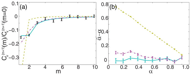
(Color online) Illustrative example of n = 1 VAC analysis of 2D simulated data for D^* = 0.01μm²/s^α, t_E = 10 ms, p̄ = 1000, and b = 0. The ensemble consisted of 100 tracks of length 100 frames each. Offsets due to static error have been removed by first estimating σ₀ for the specified photon statistics. Error bars reflect the S.E.M. from 100 bootstrapped samples of the ensemble. In both panels the gold dashed line corresponds to the VAC without inclusion of dynamic error, the magenta dashed-dotted line corresponds to the intermediate treatment of dynamic error as described in the text, and the cyan solid line corresponds to the full treatment of dynamic error. (a) Example computed VAC for α = 0.2 (black dots and error bars) and the corresponding predicted curves for each treatment of dynamic error. The point at m = 1 is not plotted for the sake of scaling the figure and since each scaled VAC is equal to 1 here by definition. (b) Bias in the estimate of α for various α.

III. CONCLUSIONS

By thoroughly analyzing data from tracked chromosomal loci in live yeast we found that both static and dynamic errors must be properly accounted for when considering anomalous diffusion. Tracking the same particles in two channels with different static error was shown to be particularly useful in demonstrating the need for the full analysis. We thus showed that when the static error has been effectively mitigated, one must still include the effects of dynamic error in order to infer the correct parameters of motion. For the MSD, this means that the complete expression in Eq. (8) should be applied. For analysis of the VAC we derived Eqs. (20)–(22). We note that recently proposed analytical methods based on maximum likelihood [13] and covariance-based estimation [14] are directly related to the VAC, and so versions of Eqs. (20)–(22) will be necessary to properly generalize these approaches beyond pure Brownian motion.

The expected values of MSD and VAC reported here are clearly useful, as they compare well to our experimental data. Future work should extend these results to derive the full distributions of the ensemble, which also depend on sampling statistics. To this end it is simple to set up the derivation of higher moments, but it quickly becomes difficult to maintain analytical tractability. Future work should also include non-stationary and nonergodic effects, for instance, due to confinement or underdamped fractional Langevin behavior [57].

The equations presented were derived assuming FBM and its defining covariance function, Eq. (3). This framework is appropriate for our purposes since our chromosomal loci data displayed the characteristic VAC of the form in Eq. (16). The latter fact certainly distinguishes the source of anomaly from confined diffusion or continuous time random walk, as shown in previous work [28,54,55]. The identification of FBM in our data is also consistent with previous tracking studies of chromosomal loci in other organisms [12,31,48]. We note that previous work suggests that obstructed diffusion can also lead to negative signatures in the VAC, and that the non-Gaussianity of the corresponding increments can be difficult to detect [55,58]. However, our data not only display negative signatures in the VAC, but fit well to the specific form of Eq. (16) consistent with FBM. If another source of anomaly happens to produce the correlations of Eq. (16), then our derived Eqs. (20)–(22) still hold, much in the same way that Eq. (8) holds for any motion of the correct power-law MSD scaling [17].

IV. METHODS FOR EXPERIMENTAL DATA ANALYSIS

Details on the strain construction and growth, microscopy, and image analysis can be found in [39]. MSDs and VACs were produced by calculating the time-averaged version for each individual trajectory. Then the results from individual trajectories were averaged together before any fitting. For our experimental data we used the MATLAB function trimmean to ignore the maximum and minimum 5% of the values when computing the ensemble mean. This was done because we noted that a few outliers exhibited abrupt, very large jumps in only the x direction, which caused inflated MSDs and α only in this direction. These large, abrupt jumps are indicative of some heterogeneous behavior and perhaps a short-lived active process. They should be investigated in future work, but here they were removed such that the x, y, and z data were equivalent in their ensemble means. In the interest of symmetry, this approach also removed small outliers before fitting, though the effect of this was less drastic. We produced estimated parameters by fitting the ensemble and time-averaged curves to the equations described using the MATLAB function lsqnonlin. In estimating parameters we imposed physically reasonable yet modest lower and upper bounds, mostly in order to ensure non-negative numbers. In particular, in fitting the MSD of our chromosomal loci we constrained α to (0, 2), D^* to (10⁻⁵, 10³)μm²/s^α, and σ to (0, 10) μm. This least-squares fitting was carried out in log space, i.e., the minimization function was of the form [log(data)–log(model)]². We found that doing the fit in log space put the correct emphasis on the early time points, which (1) are better averaged and thus more reliable and (2) best capture the error effects we emphasize. Also, this gives the most direct connection to the usual treatment in the absence of errors.

References

- 1.Peterman EJ, Sosa H, Moerner WE. Single-molecule fluorescence spectroscopy and microscopy of biomolecular motors. Annu Rev Phys Chem. 2004;55:79. doi: 10.1146/annurev.physchem.55.091602.094340. [DOI] [PubMed] [Google Scholar]
- 2.Saxton MJ, Jacobson K. Single-particle tracking: Applications to membrane dynamics. Annu Rev Biophys Biomol Struct. 1997;26:373. doi: 10.1146/annurev.biophys.26.1.373. [DOI] [PubMed] [Google Scholar]
- 3.Ritchie K, Shan X, Kondo J, Iwasawa K, Fujiwara T, Kusumi A. Detection of non-brownian diffusion in the cell membrane in single molecule tracking. Biophys J. 2005;88:2266. doi: 10.1529/biophysj.104.054106. [DOI] [PMC free article] [PubMed] [Google Scholar]
- 4.Vrljic M, Nishimura SY, Brasselet S, Moerner WE, McConnell HM. Translational diffusion of individual class II MHC membrane proteins in cells. Biophys J. 2002;83:2681. doi: 10.1016/S0006-3495(02)75277-6. [DOI] [PMC free article] [PubMed] [Google Scholar]
- 5.Umemura YM, Vrljic M, Nishimura SY, Fujiwara TK, Suzuki KGN, Kusumi A. Both MHC class II and its GPI-anchored form undergo hop diffusion as observed by single-molecule tracking. Biophys J. 2008;95:435. doi: 10.1529/biophysj.107.123018. [DOI] [PMC free article] [PubMed] [Google Scholar]
- 6.Tolić-Nørrelykke IM, Munteanu E-L, Thon G, Oddershede L, Berg-Sørensen K. Anomalous diffusion in living yeast cells. Phys Rev Lett. 2004;93:078102. doi: 10.1103/PhysRevLett.93.078102. [DOI] [PubMed] [Google Scholar]
- 7.Golding I, Cox EC. Physical nature of bacterial cytoplasm. Phys Rev Lett. 2006;96:098102. doi: 10.1103/PhysRevLett.96.098102. [DOI] [PubMed] [Google Scholar]
- 8.Weber SC, Spakowitz AJ, Theriot JA. Nonthermal ATP-dependent fluctuations contribute to the in vivo motion of chromosomal loci. Proc Natl Acad Sci USA. 2012;109:7338. doi: 10.1073/pnas.1119505109. [DOI] [PMC free article] [PubMed] [Google Scholar]
- 9.Javer A, Long Z, Nugent E, Grisi M, Siriwatwetchakul K, Dorfman KD, Cicuta P, Lagomarsino MC. Short-time movement of E. Coli chromosomal loci depends on coordinate and subcellular localization. Nat Commun. 2013;4:3003. doi: 10.1038/ncomms3003. [DOI] [PubMed] [Google Scholar]
- 10.Bronstein I, Israel Y, Kepten E, Mai S, Shav-Tal Y, Barkai E, Garini Y. Transient anomalous diffusion of telomeres in the nucleus of mammalian cells. Phys Rev Lett. 2009;103:018102. doi: 10.1103/PhysRevLett.103.018102. [DOI] [PubMed] [Google Scholar]
- 11.Cabal GG, Genovesio A, Rodriguez-Navarro S, Zimmer C, Gadal O, Lesne A, Buc H, Feuerbach-Fournier F, Olivo-Marin J, Hurt ED. SAGA interacting factors confine sub-diffusion of transcribed genes to the nuclear envelope. Nature. 2006;441:770. doi: 10.1038/nature04752. [DOI] [PubMed] [Google Scholar]
- 12.Burnecki K, Kepten E, Janczura J, Bronshtein I, Garini Y, Weron A. Universal algorithm for identification of fractional Brownian motion. A case of telomere subdiffusion. Biophys J. 2012;103:1839. doi: 10.1016/j.bpj.2012.09.040. [DOI] [PMC free article] [PubMed] [Google Scholar]
- 13.Berglund AJ. Statistics of camera-based single-particle tracking. Phys Rev E. 2010;82:011917. doi: 10.1103/PhysRevE.82.011917. [DOI] [PubMed] [Google Scholar]
- 14.Vestergaard CL, Blainey PC, Flyvbjerg H. Optimal estimation of diffusion coefficients from single-particle trajectories. Phys Rev E. 2014;89:022726. doi: 10.1103/PhysRevE.89.022726. [DOI] [PubMed] [Google Scholar]
- 15.Qian H, Sheetz MP, Elson EL. Single particle tracking. Analysis of diffusion and flow in two dimensional systems. Biophys J. 1991;60:910. doi: 10.1016/S0006-3495(91)82125-7. [DOI] [PMC free article] [PubMed] [Google Scholar]
- 16.Jeon J, Metzler R. Analysis of short subdiffusive time series: Scatter of the time-averaged mean-squared displacement. J Phys A: Math Theor. 2010;43:252001. [Google Scholar]
- 17.Savin T, Doyle PS. Static and dynamic errors in particle tracking microrheology. Biophys J. 2005;88:623. doi: 10.1529/biophysj.104.042457. [DOI] [PMC free article] [PubMed] [Google Scholar]
- 18.Martin DS, Forstner MB, Käs JA. Apparent subdiffusion inherent to single particle tracking. Biophys J. 2002;83:2109. doi: 10.1016/S0006-3495(02)73971-4. [DOI] [PMC free article] [PubMed] [Google Scholar]
- 19.Kepten E, Bronshtein I, Garini Y. Improved estimation of anomalous diffusion exponents in single-particle tracking experiments. Phys Rev E. 2013;87:052713. doi: 10.1103/PhysRevE.87.052713. [DOI] [PubMed] [Google Scholar]
- 20.Hellmann M, Klafter J, Heermann DW, Weiss M. Challenges in determining anomalous diffusion in crowded fluids. J Phys: Condens Matter. 2011;23:234113. doi: 10.1088/0953-8984/23/23/234113. [DOI] [PubMed] [Google Scholar]
- 21.Michalet X, Berglund AJ. Optimal diffusion coefficient estimation in single-particle tracking. Phys Rev E. 2012;85:061916. doi: 10.1103/PhysRevE.85.061916. [DOI] [PMC free article] [PubMed] [Google Scholar]
- 22.Michalet X. Mean square displacement analysis of single-particle trajectories with localization error: Brownian motion in an isotropic medium. Phys Rev E. 2010;82:041914. doi: 10.1103/PhysRevE.82.041914. [DOI] [PMC free article] [PubMed] [Google Scholar]
- 23.Deschout H, Neyts K, Braeckmans K. The influence of movement on the localization precision of subresolution particles in fluorescence microscopy. J Biophotonics. 2012;5:97. doi: 10.1002/jbio.201100078. [DOI] [PubMed] [Google Scholar]
- 24.Saxton MJ. Anomalous diffusion due to obstacles: A Monte Carlo study. Biophys J. 1994;66:394. doi: 10.1016/s0006-3495(94)80789-1. [DOI] [PMC free article] [PubMed] [Google Scholar]
- 25.Scher H, Montroll EW. Anomalous transit-time dispersion in amorphous solids. Phys Rev B. 1975;12:2455. [Google Scholar]
- 26.Mandelbrot BB, Van Ness JW. Fractional Brownian motions, fractional noises and applications. SIAM Rev. 1968;10:422. [Google Scholar]
- 27.Ernst D, Köhler J, Weiss M. Probing the type of anomalous diffusion with single-particle tracking. Phys Chem Chem Phys. 2014;16:7686. doi: 10.1039/c4cp00292j. [DOI] [PubMed] [Google Scholar]
- 28.Weber SC, Thompson MA, Moerner WE, Spakowitz AJ, Theriot JA. Analytical tools to distinguish the effects of localization error, confinement, and medium elasticity on the velocity autocorrelation function. Biophys J. 2012;102:2443. doi: 10.1016/j.bpj.2012.03.062. [DOI] [PMC free article] [PubMed] [Google Scholar]
- 29.Szymanski J, Weiss M. Elucidating the origin of anomalous diffusion in crowded fluids. Phys Rev Lett. 2009;103:038102. doi: 10.1103/PhysRevLett.103.038102. [DOI] [PubMed] [Google Scholar]
- 30.Condamin S, Tejedor V, Voituriez R, Bénichou O, Klafter J. Probing microscopic origins of confined subdiffusion by first-passage observables. Proc Natl Acad Sci USA. 2008;105:5675. doi: 10.1073/pnas.0712158105. [DOI] [PMC free article] [PubMed] [Google Scholar]
- 31.Kepten E, Bronshtein I, Garini Y. Ergodicity convergence test suggests telomere motion obeys fractional dynamics. Phys Rev E. 2011;83:041919. doi: 10.1103/PhysRevE.83.041919. [DOI] [PubMed] [Google Scholar]
- 32.Tejedor V, Bénichou O, Voituriez R, Jungmann R, Simmel F, Selhuber-Unkel C, Oddershede LB, Metzler R. Quantitative analysis of single particle trajectories: Mean maximal excursion method. Biophys J. 2010;98:1364. doi: 10.1016/j.bpj.2009.12.4282. [DOI] [PMC free article] [PubMed] [Google Scholar]
- 33.Jeon JH, Metzler R. Fractional Brownian motion and motion governed by the fractional Langevin equation in confined geometries. Phys Rev E. 2010;81:021103. doi: 10.1103/PhysRevE.81.021103. [DOI] [PubMed] [Google Scholar]
- 34.Burnecki K, Muszkieta M, Sikora G, Weron A. Statistical modelling of subdiffusive dynamics in the cytoplasm of living cells: A FARIMA approach. Europhys Lett. 2012;98:10004. [Google Scholar]
- 35.Magdziarz M, Weron A, Burnecki K, Klafter J. Fractional Brownian motion versus the continuous-time random walk: A simple test for subdiffusive dynamics. Phys Rev Lett. 2009;103:180602. doi: 10.1103/PhysRevLett.103.180602. [DOI] [PubMed] [Google Scholar]
- 36.Metzler R, Jeon J, Cherstvy AG, Barkai E. Anomalous diffusion models and their properties: Non-stationarity, non-ergodicity, and ageing at the centenary of single particle tracking. Phys Chem Chem Phys. 2014;16:24128. doi: 10.1039/c4cp03465a. [DOI] [PubMed] [Google Scholar]
- 37.Casolari JM, Brown CR, Komili S, West J, Hieronymus H, Silver PA. Genome-wide localization of the nuclear transport machinery couples transcriptional status and nuclear organization. Cell. 2004;117:427. doi: 10.1016/s0092-8674(04)00448-9. [DOI] [PubMed] [Google Scholar]
- 38.Straight AF, Belmont AS, Robinett CC, Murray AW. GFP tagging of budding yeast chromosomes reveals that protein-protein interactions can mediate sister chromatid cohesion. Curr Biol. 1996;6:1599. doi: 10.1016/s0960-9822(02)70783-5. [DOI] [PubMed] [Google Scholar]
- 39.Backlund MP, Joyner R, Weis K, Moerner WE. Correlations of three-dimensional motion of chromosomal loci in yeast revealed by the double-helix point spread function microscope. Mol Biol Cell. 2014;25:3619. doi: 10.1091/mbc.E14-06-1127. [DOI] [PMC free article] [PubMed] [Google Scholar]
- 40.Pavani SRP, Thompson MA, Biteen JS, Lord SJ, Liu N, Twieg RJ, Piestun R, Moerner WE. Three-dimensional, single-molecule fluorescence imaging beyond the diffraction limit by using a double-helix point spread function. Proc Natl Acad Sci USA. 2009;106:2995. doi: 10.1073/pnas.0900245106. [DOI] [PMC free article] [PubMed] [Google Scholar]
- 41.Thompson MA, Casolari JM, Badieirostami M, Brown PO, Moerner WE. Three-dimensional tracking of single mRNA particles in Saccharomyces cerevisiae using a double-helix point spread function. Proc Natl Acad Sci USA. 2010;107:17864. doi: 10.1073/pnas.1012868107. [DOI] [PMC free article] [PubMed] [Google Scholar]
- 42.Gahlmann A, Ptacin JL, Grover G, Quirin S, von Diezmann ARS, Lee MK, Backlund MP, Shapiro L, Piestun R, Moerner WE. Quantitative multicolor subdiffraction imaging of bacterial protein ultrastructures in 3D. Nano Lett. 2013;13:987. doi: 10.1021/nl304071h. [DOI] [PMC free article] [PubMed] [Google Scholar]
- 43.Gahlmann A, Moerner WE. Exploring bacterial cell biology with single-molecule tracking and super-resolution imaging. Nat Rev Microbiol. 2014;12:9. doi: 10.1038/nrmicro3154. [DOI] [PMC free article] [PubMed] [Google Scholar]
- 44.Destainville N, Salome L. Quantification and correction of systematic errors due to detector time-averaging in single-molecule tracking experiments. Biophys J. 2006;90:L17. doi: 10.1529/biophysj.105.075176. [DOI] [PMC free article] [PubMed] [Google Scholar]
- 45.Savin T, Doyle PS. Role of a finite exposure time on measuring an elastic modulus using microrheology. Phys Rev E. 2005;71:041106. doi: 10.1103/PhysRevE.71.041106. [DOI] [PubMed] [Google Scholar]
- 46.See Supplemental Material at http://link.aps.org/supplemental/10.1103/PhysRevE.xx.xxxxxx for [give brief description of material].
- 47.Kou SC, Xie XS. Generalized Langevin equation with fractional Gaussian noise: Subdiffusion within a single protein molecule. Phys Rev Lett. 2004;93:180603. doi: 10.1103/PhysRevLett.93.180603. [DOI] [PubMed] [Google Scholar]
- 48.Weber SC, Spakowitz AJ, Theriot JA. Bacterial chromosomal loci move subdiffusively through a viscoelastic cytoplasm. Phys Rev Lett. 2010;104:238102. doi: 10.1103/PhysRevLett.104.238102. [DOI] [PMC free article] [PubMed] [Google Scholar]
- 49.Jeon JH, Tejedor V, Burov S, Barkai E, Selhuber-Unkel C, Berg-Sørensen K, Oddershede L, Metzler R. In vivo anomalous diffusion and weak ergodicity breaking of lipid granules. Phys Rev Lett. 2011;106:048103. doi: 10.1103/PhysRevLett.106.048103. [DOI] [PubMed] [Google Scholar]
- 50.Deng W, Barkai E. Ergodic properties of fractional Brownian-Langevin motion. Phys Rev E. 2009;79:011112. doi: 10.1103/PhysRevE.79.011112. [DOI] [PubMed] [Google Scholar]
- 51.Kroese DP, Botev ZI. Lecture Notes in Mathematics. Vol. 2120. Springer International Publishing; Switzerland: 2015. Stochastic Geometry, Spatial Statistics, and Random Fields; pp. 369–404. [Google Scholar]
- 52.Thompson RE, Larson DR, Webb WW. Precise nanometer localization analysis for individual fluorescent probes. Biophys J. 2002;82:2775. doi: 10.1016/S0006-3495(02)75618-X. [DOI] [PMC free article] [PubMed] [Google Scholar]
- 53.Mortensen KI, Churchman LS, Spudich JA, Flyvbjerg H. Optimized localization analysis for single-molecule tracking and super-resolution microscopy. Nat Methods. 2010;7:377. doi: 10.1038/nmeth.1447. [DOI] [PMC free article] [PubMed] [Google Scholar]
- 54.Weber SC, Theriot JA, Spakowitz AJ. Subdiffusive motion of a polymer composed of subdiffusive monomers. Phys Rev E. 2010;82:011913. doi: 10.1103/PhysRevE.82.011913. [DOI] [PMC free article] [PubMed] [Google Scholar]
- 55.Weiss M. Single-particle tracking data reveal anticorrelated fractional Brownian motion in crowded fluids. Phys Rev E. 2013;88:010101. doi: 10.1103/PhysRevE.88.010101. [DOI] [PubMed] [Google Scholar]
- 56.Cohen AE. PhD thesis. Stanford University; 2006. Trapping and manipulating single molecules in solution. [Google Scholar]
- 57.Kursawe J, Schulz J, Metzler R. Transient aging in fractional Brownian and Langevin-equation motion. Phys Rev E. 2013;88:062124. doi: 10.1103/PhysRevE.88.062124. [DOI] [PubMed] [Google Scholar]
- 58.Meroz Y, Sokolov IM, Klafter J. Test for determining a subdiffusive model in ergodic systems from single trajectories. Phys Rev Lett. 2013;110:090601. doi: 10.1103/PhysRevLett.110.090601. [DOI] [PubMed] [Google Scholar]
Associated Data
This section collects any data citations, data availability statements, or supplementary materials included in this article.