Statistical inference is a procedure that we try to make a decision about a population by using information from a sample which is a part of it. In modern statistics it is assumed that we never know about a population, and there is always a possibility to make errors. Theoretically a sample statistic may have values in a wide range because we may select a variety of different samples, which is called a sampling variation. To get practically meaningful inference we preset a certain level of error. In statistical inference we presume two types of error, type I and type II errors.
Null hypothesis and alternative hypothesis
The first step of statistical testing is the setting of hypotheses. When comparing multiple group means we usually set a null hypothesis. For example, "There is no true mean difference," is a general statement or a default position. The other side is an alternative hypothesis such as "There is a true mean difference." Often the null hypothesis is denoted as H0 and the alternative hypothesis as H1 or Ha. To test a hypothesis, we collect data and measure how much the data support or contradict the null hypothesis. If the measured results are similar to or only slightly different from the condition stated by the null hypothesis, we do not reject and accept H0. However, if the dataset shows a big and significant difference from the condition stated by the null hypothesis, we regard that there is enough evidence that the null hypothesis is not true and reject H0. When a null hypothesis is rejected, the alternative hypothesis is adopted.
Type I and type II errors
As we assume that we never directly know the information of the population, we never know whether the statistical decision is right or wrong. Actually, the H0 may be right or wrong and we could make a decision of the acceptance or the rejection of H0. In a situation of statistical decision, there may be four different occasions as presented in Table 1. Two situations lead correct conclusions that true H0 is accepted and false H0 is rejected. However, the others are two incorrect erroneous situations that false H0 is accepted and true H0 is rejected. A Type I error or alpha (α) error refers to an erroneous rejection of true H0. Conversely, a Type II error or beta (β) error refers to an erroneous acceptance of false H0.
Table 1. Possible results of hypothesis testing.
| Conclusion based on data | Truth | |
|---|---|---|
| H0 True | H0 False | |
| Reject H0 | Type I error (α) | Correct conclusion (Power = 1 - β) |
| Fail to reject H0 | Correct conclusion (1 - α) | Type II error (β) |
Making some level of error is unavoidable because fundamental uncertainty lies in a statistical inference procedure. As allowing errors is basically harmful, we need to control or limit the maximum level of errors. Which type of error is more risky between type I and type II errors? Traditionally, committing type I error has been considered more risky, and thus more strict control of type I error has been performed in statistical inference.
When we have interest in the null hypothesis only, we may think about type I error only. Let's consider a situation that someone develops a new method and insists that it is more efficient than conventional methods but the new method is actually not more efficient. The truth is H0 that says "The effects of conventional and newly developed methods are equal." Let's suppose the statistical test results support the efficiency of the new method, which is an erroneous conclusion that the true H0 is rejected (type I error). According to the conclusion, we consider adopting the newly developed method and making effort to construct a new production system. The erroneous statistical inference with type I error would result in an unnecessary effort and vain investment for nothing better. Otherwise, if the statistical conclusion was made correctly that the conventional and newly developed methods were equal, then we could comfortably stay with the familiar conventional method. Therefore, type I error has been strictly controlled to avoid such useless effort for an inefficient change to adopt new things.
In other example, let's think that we are interested in a safety issue. Someone developed a new method which is actually safer compared to the conventional method. In this situation, null hypothesis states that "Degrees of safety of both methods are equal", when the alternative hypothesis that "The new method is safer than conventional method" is true. Let's suppose that we erroneously accept the null hypothesis (type II error) as the result of statistical inference. We erroneously conclude equal safety and we stay on the less safe conventional environment and have to be exposed to risks continuously. If the risk is a serious one, we would stay in a danger because of the erroneous conclusion with type II error. Therefore, not only type I error but also type II error need to be controlled.
Schematic example of type I and type II errors
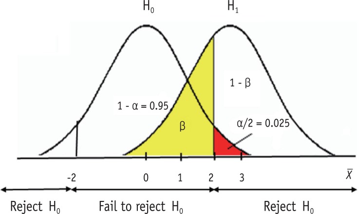
Figure 1 shows a schematic example of relative sampling distributions under a null hypothesis (H0) and an alternative hypothesis (H1). Let's suppose they are two sampling distributions of sample means (X). H0 states that sample means are normally distributed with population mean zero. H1 states the different population mean of 3 under the same shape of sampling distribution. For simplicity, let's assume the standard error of two distributions is one. Therefore, the sampling distribution under H0 is assumed as the standard normal distribution in this example. In statistical testing on H0 with an alpha level 0.05, the critical values are set at ± 2 (or exactly 1.96). If the observed sample mean from the dataset lies within ± 2, then we accept H0, because we don't have enough evidence to deny H0. Or, if the observed sample mean lies beyond the range, we reject H0 and adopt H1. In this example we can say that the probability of alpha error (two-sided) is set at 0.05, because the area beyond ± 2 is 0.05, which is the probability of rejecting the true H0. As seen in Figure 1, extreme values larger than absolute 2 can appear under H0 with the standard normal distribution ranging to infinity. However, we practically decide to reject H0, because the extreme values are too different from the assumed mean, zero. Though the decision includes a probability of error of 0.05, we allow the risk of error because the difference is considered sufficiently big to reach a reasonable conclusion that the null hypothesis is false. As we never know the truth whether the sample dataset we have is from the population H0 or H1, we can make decision only based on the value we observe from the sample data.
Figure 1. Illustration of type I (α) and type II (β) errors.
Type II error is shown as the area lower than 2 under the distribution of H1. The amount of type II error can be calculated only when the alternative hypothesis suggest a definite value. In Figure 1, a definite mean value of 3 is used in the alternative hypothesis. The critical value 2 is one standard error (= 1) smaller than mean 3 and is standardized to in a standard normal distribution. The area less than z = -1 is 0.16 (yellow area) in standard normal distribution. Therefore, the amount of type II error is obtained as 0.16 in this example.
Relationship and affecting factors on type I and type II errors
1. Related change of both errors
Type I and type II errors are closely related. If all other conditions are the same, the reduction of Type I error level accompanies the increase of type II error level. When we decrease alpha error level from 0.05 to 0.01, the critical value moves outward to around ± 2.58. As the result, beta level will increase to around 0.34 in Figure 1, if all other conditions are the same. Conversely, moving the determinant line to the left side will cause both decrease of type II error level and increase of type I error level. Therefore, the determination of error level should be a procedure considering both error types simultaneously.
2. Effect of distance between H0 and H1
If H1 suggest a bigger center, e.g., 4 instead of 3, then the distribution moves to the right. If we fix the alpha level as 0.05, then the beta level gets smaller than ever. If the center value is 4 then z value is -2 and the area less than -2 in the standard normal distribution is obtained as 0.025. If all other condition is the same, the increase of distance between H0 and H1 decrease the beta error level.
3. Effect of sample size
Then how do we maintain both error levels lower? Increasing the sample size is one answer, because a large sample size reduce standard error (standard deviation/√sample size) when all other conditions retained as the same. Smaller standard error can produce more concentrated sampling distributions with slender curve under both null and alternative hypothesis and the consequent overlapping area gets smaller. As sample size increases, we can get satisfactory low levels of both alpha and beta errors.
Statistical significance level
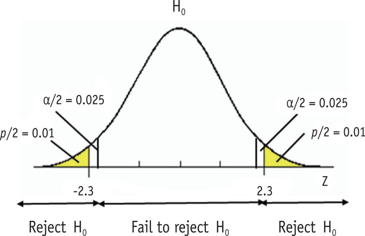
Type I error level of is often called a significance level. In a statistical testing, we reject the null hypothesis when the observed value from the dataset is located in area of extreme 0.05 and conclude there is evidence of difference from the null hypothesis when we set the alpha level at 0.05. As we consider the difference over the level is statistically significant, the level is called a significance level. Sometimes the significance level is expressed using p value, e.g., "Statistical significance was determined as p < 0.05." P value is defined as the probability of obtaining the observed value or more extreme values when the null hypothesis is true. Figure 2 shows that type I error level at 0.05 and a two-sided p value of 0.02. The observed z value 2.3 was located in the rejection region with p value of 0.02, which is smaller than the significance level 0.05. Small p value indicates that the probability of observing such a dataset or more extreme cases is very low under the assumed null hypothesis.
Figure 2. Significance level and p value.
Statistical power
Power is the probability of rejecting a false null hypothesis, which is the other side of type II error. Power is calculated as 1- Type II error (β). In Figure 1, type II error level is 0.16 and power is obtained as 0.84. Usually a power level of 0.8 - 0.9 is required in experimental studies. Because of the relationship between type I and type II errors, we need to keep a minimum required level of both errors. Sufficient sample size is needed to keep the type I error low as 0.05 or 0.01 and the power high as 0.8 or 0.9.
References
- 1.Rosner B. Fundamentals of Biostatistics. 6th ed. Belmont: Duxbury Press; 2006. pp. 226–252. [Google Scholar]


