Quantitative Evaluation of Models for Solvent-based, On-column Focusing in Liquid Chromatography

Abstract

On-column focusing or preconcentration is a well-known approach to increase concentration sensitivity by generating transient conditions during the injection that result in high solute retention. Preconcentration results from two phenomena: 1) solutes are retained as they enter the column. Their velocities are k′-dependent and lower than the mobile phase velocity and 2) zones are compressed due to the step-gradient resulting from the higher elution strength mobile phase passing through the solute zones. Several workers have derived the result that the ratio of the eluted zone width (in time) to the injected time width is the ratio k₂/k₁ where k₁ is the retention factor of a solute in the sample solvent and k₂ is the retention factor in the mobile phase (isocratic). Mills et al. proposed a different factor. To date, neither of the models has been adequately tested. The goal of this work was to evaluate quantitatively these two models. We used n-alkyl esters of p-hydroxybenzoic acid (parabens) as solutes. By making large injections to create obvious volume overload, we could measure accurately the ratio of widths (eluted/injected) over a range of values of k₁ and k₂. The Mills et al. model does not fit the data. The data are in general agreement with the factor k₂/k₁, but focusing is about 10% better than the prediction. We attribute the extra focusing to the fact that the second, compression, phenomenon provides a narrower zone than that expected for the passage of a step gradient through the zone.

1. Introduction

In most analytical chromatographic analyses, the injected volume of sample is much smaller than the volume of mobile phase carrying a peak out of the column (the peak volume). In this case, the amount of sample injected affects the peak height linearly, but has no effect on the peak width. If the volume of sample injected is increased to enhance concentration detection limits, at some point the eluting peak will become broadened. This phenomenon is now termed volume overload. It is worth noting that a very accurate picture of this phenomenon was published in 1956 by van Deemter et al. using gas chromatography [1]. Sternberg later put this effect into rigorous mathematical terms by explaining that volume overload leads to a peak shape that is a convolution of the peak shape observed with a small-volume injection and the rectangular concentration-distance profile as injected [2]. The former can be determined from a small-volume injection. The latter comes from the fact that the length of the zone of solute on the column once the injection is complete is smaller by the factor 1/(1+k′) than the length of the column occupied by the injected solvent. Further, Sternberg pointed out that the variance of the resulting peak was the sum of the variances of the two functions. It becomes a simple matter to calculate the maximum injected volume that leads to an acceptable increase in peak width. Injecting this volume will lead to the highest concentration sensitivity with minimal (tolerable) impact on separation quality.

When the sample liquid is a weaker chromatographic solvent than the mobile phase, analyte retention on the stationary phase is higher, increasing the allowable injected volume in comparison to the allowable volume when the sample liquid is the mobile phase. This phenomenon, often called on-column focusing or preconcentration, is used routinely in capillary LC (cLC) where the injection of low nL-scale volumes is required to avoid volume overload when injecting samples made in mobile phase [3–6]. On-column focusing is not limited to cLC, it can be used to advantage with any size column [7, 8] or application from trace analysis to two-dimensional LC [9–15]. On-column focusing also happens quite often as a natural consequence of gradient elution chromatography because many solutes are highly retained in the relatively weak initial solvent composition as described by Snyder [16]. He described an additional effect that occurs in gradient elution, namely, the peak compression of the already focused band that results because the tail of the injected band moves with the stronger solvent for a longer time than the front of the band. As our current interest is in isocratic elution with on-column focusing followed by peak compression due to the introduction of the stronger mobile phase, we will discuss the problem in the context of a step gradient. Thus, there are two factors to consider in solvent-based on-column focusing: one relates to the retention factor of the solute as it is injected and the other is due to the compression occurring when the mobile phase is stronger than the injected sample’s liquid. In the following discussion, we do not consider the case where mass overload contributes to bandspreading.

Several groups have contributed to the understanding of these phenomena. Snyder’s work has been mentioned [17, 18]. Later, the Poppe group combined the on-column focusing and the step-gradient-induced compression in the context of a precolumn trapping column/backflush for analytical work [19, 20]. They arrived at the simple result that the solute elutes from the column in a volume that is a factor k₂/k₁ smaller than the injected volume, where k₁ is the solute retention factor in the sample solvent and k₂ is the retention factor in the mobile phase. Here, for simplicity column dynamics-induced bandspreading was ignored. Hartwick, and subsequently the Desmet group found the same relationship for post-column peak trapping/concentration and elution [21–23]. The same relationship was found for preconcentration in CEC [24].

Mills et al. [25] also derived a factor for preconcentration resulting from the step gradient using a vaguely described function of k₁ and k₂ in Slais et al. [26]. Rather than finding the factor k₂/k₁ they found the factor ${\left(\frac{1+k_2}{1+k_1}\right)}^2$. This predicts rather large focusing effects. For instance, if k₁ = 50 and k₂ = 5, the former relationship predicts that the eluted volume would be 10 times smaller than the injected volume while Mills et al.’s relationship predicts that the eluted volume would be 72 times smaller than the injected volume.

Unfortunately, no quantitative evaluation of these relationships exists. The rationale for focusing is to increase sensitivity, so a natural quantitative test is to determine the sensitivity enhancement from these processes. Numerically, the sensitivity enhancement is the inverse of the ratios discussed in the last paragraph. However, peak height is strongly influenced by on- column bandspreading which depends on numerous phenomena. As a result, predicted sensitivity enhancements that do not take into account on-column dynamic bandspreading will be optimistic so they cannot themselves form the basis for a quantitative evaluation of a model. Another approach to testing these predictions is to calculate a volume that can be injected without significant volume overload and then test this experimentally. This approach requires a knowledge of the number of theoretical plates, N, experienced by each solute in the absence of volume overload, a knowledge of the shape of the injected volume (in order to estimate its variance contribution to the overall peak variance), as well as a quantitative assertion of the fractional loss in N that the chromatographer is willing to accept. Because of these factors, this approach also cannot quantitatively confirm the expected result despite its significant practical significance.

In this work, we first recapitulate the simple theoretical derivation of the k₂/k₁ focusing factor. As described above, there are several extant publications reciting the same result. However it is important to show clearly how this result occurs as a part of this discussion. We have designed an experiment in which we attempt to experimentally validate this relationship by measuring peak width rather than peak height. As the objective is to determine accurately the ratio of eluted volume to injected volume, we create eluted volumes significantly greater than the natural peak volume. This is in contrast to the work cited above where the objective was to demonstrate the utility of on-column focusing to enhance sensitivity in analytical determinations, not the validity of the model. Using accurately determined experimental retention factors and measurements of the injection band width we comment on the validity of the k₂/k₁ factor and its practical application to increase analysis sensitivity in liquid chromatography.

2. Theory

2.1 Derivation of the k₂/k₁ factor

Consider a zone of solute of volume V_inj injected into a column. During the injection the relative volumes of the sample and the column suffice to cause the sample liquid itself to be the mobile phase transiently during sample loading. The discussion that follows will consider the on-column length occupied by the injected volume. Fig. 1 illustrates the process schematically. At t = 0 a volume V_inj passes from the loop onto the column. The solute will occupy a length ℓ₁ on the column given by Eq. 1 in which the injection time, t_inj is multiplied by the average zone velocity. The former is V_inj/F where F is flow rate, while the latter is the determined by the average mobile phase velocity v_mp and k₁ the retention factor for the solute in the sample liquid acting as mobile phase.

Figure 1.

Schematic describing the effect of solvent-based on-column focusing. Compression of the injection zone results from the increased retention at the head of the column in the sample solvent and the step-gradient resulting from the higher elution strength mobile phase passing through the injection plug.

$${\ell }_1=\left(\frac{V_{\mathit{inj}}}{F}\right)\frac{v_{mp}}{1+k_1}=t_{\mathit{inj}}\frac{v_{mp}}{1+k_1}$$ Eq. 1

As the mobile phase passes through the sample band the step gradient that follows compresses the zone further. Additional compression results because the stronger elution strength mobile phase moves the tail of the zone for a longer time than it moves the front. We will thus determine how far the tail of the zone moves, Δℓ_t, and how far the front of the zone moves, Δℓ_f, in the time that it takes for the mobile phase to reach the front of the zone, t₁. Once the mobile phase reaches the front of the zone, there is no further compression by the step gradient. The time, t₁, that the mobile phase requires to reach the moving front of the zone is given by a distance into the column, ℓ₂ and the velocity v_mp. The distance ℓ₂ (Fig. 1) is the initial length of the compressed zone plus the additional distance moved at the front,

$${\ell }_2=t_1{v}_{mp}={\ell }_1+\mathrm{\Delta }{\ell }_f$$ Eq. 2

During time t₁, the front moves at a velocity v_mp/(1+k₁). Thus, the distance the front moves in time t₁ is

$$\mathrm{\Delta }{\ell }_f=t_1\frac{v_{mp}}{1+k_1}$$ Eq. 3

Replacing ℓ₁ in Eq. 2 with Eq. 1 and Δℓ_f with Eq. 3 and rearranging leads to Eq. 4.

$$t_1=\frac{t_{\mathit{inj}}}{k_1}$$ Eq. 4

During this time, the front moves a distance equal to its velocity multiplied by t₁:

$$\mathrm{\Delta }{\ell }_f=\frac{v_{mp}}{1+k_1}\frac{t_{\mathit{inj}}}{k_1}$$ Eq. 5

As the tail moves at a velocity v_mp/(1+k₂), the distance that it moves, Δℓ_t, is t₁ times this velocity:

$$\mathrm{\Delta }{\ell }_t=t_1\frac{v_{mp}}{1+k_2}=\frac{v_{mp}}{1+k_2}\frac{t_{\mathit{inj}}}{k_1}$$ Eq. 6

The width of the zone on the column is thus the initial width minus the distance traveled by the tail plus the distance traveled by the front

$$W={\ell }_1-\mathrm{\Delta }{\ell }_t+\mathrm{\Delta }{\ell }_f$$ Eq. 7

$$=t_{\mathit{inj}}{v}_{mp}\left(\frac{1}{1+k_1}-\frac{1}{(1+k_2)k_1}+\frac{1}{(1+k_1)k_1}\right)$$ Eq. 8

When eluted, the band expands by the factor (1 + k₂). The width in time of the eluted zone is thus

$$t_{\mathit{obs}}=t_{\mathit{inj}}\left(\frac{1+k_2}{1+k_1}-\frac{1}{k_1}+\frac{1+k_2}{(1+k_1)k_1}\right)$$ Eq. 9

Simplification leads to the remarkably simple Eq.10, matching the factor derived by the groups mentioned above.

$$t_{\mathit{obs}}=t_{\mathit{inj}}\frac{k_2}{k_1}$$ Eq. 10

We can break Eq. 10 down into two components, one from the initial focusing of the injected zone as shown in Eq. 1 and one from the compression that results. In the absence of this compression effect, the on-column width of the injected solute zone is given by Eq. 1. That on-column width remains unchanged in this compression-free model. Of course, bandspreading occurs, but here we just consider the volume overload portion of the problem. In addition, as explained below in Section 2.2, the zone width is somewhat independent of mass-transport-based bandspreading. When the zone is eluted, its width in time units, t_obs, is the length, ℓ₁, divided by the velocity which is now dependent on k₂.

$$t_{\mathit{obs}}=t_{\mathit{inj}}\frac{v_{mp}}{1+k_1}\frac{1+k_2}{v_{mp}}=t_{\mathit{inj}}\frac{1+k_2}{1+k_1}$$ Eq. 11

By comparison of Eqs. 10 and 11, it can be seen that the effect of compression alone is

$$\frac{k_2}{k_1}\frac{1+k_1}{1+k_2}$$ Eq. 12

In summary, the width in time of the eluted zone resulting from an injection large enough to create obvious volume overload is expected to be the factor k₂/k₁ times the injection time. This factor is the product of two factors. One is the initial band focusing due to retention of the solute in the injected solvent, namely Eq. 11. The other is the factor due to compression of this zone by the step gradient, Eq. 12.

2.2 The eluted peak width is a robust measure of the on-column focusing effect

Our data treatment will compare the eluted width in time of obviously volume-overloaded peaks to the injection width in time. What is the best measure of “eluted width in time”? As Sternberg has explained [2] and Burke showed [27] the injection of a large volume leads to a “peak” that is the convolution of the transfer function of the chromatographic system and the injected concentration profile. This process is shown schematically in Fig. 2; see figure captions for details. In the simplest case, the latter is a rectangular function, 2B. The transfer function of the chromatographic system (Fig. 2A) is represented by the eluted concentration profile, or peak, resulting from an injection of a volume that is much smaller than the column volume. When the baseline width of the peak is smaller than the width of the rectangle, the eluted concentration profile has a flat top with its leading and trailing edges having a sigmoidal shape, 2C. When the peak is also Gaussian, the leading and trailing edges have the shape of an error function complement and error function, respectively (see Fig. S4 and S5 for experimental examples). It is important to note that when the chromatographic transfer function is symmetrical and the eluted concentration profile has a plateau then the peak width at half height is independent of the chromatographic system transfer function. Thus, increasing the width of the transfer function, e.g., by greater on-column bandspreading, does not change the width at half height. On the other hand, the variance of the eluted band does increase as the bandspreading variance increases.

Figure 2.

Simulated signals for the eluted injection profile corresponding to the convolution of the column transfer function and rectangular injection profile. Panel A shows an exponentially modified Gaussian signal resulting from on-column bandspreading (σ = 0.75 s, τ = 1 s, α_5% = 2.8); panel B a 15 s wide rectangular injection profile. Panel C shows the peak shape resulting from the convolution of the signals in panels A and B in blue. The black dashed trace is used to overlay the 15 s wide injection profile on the convolved signal illustrating the potential utility of the half width metric to quantitatively evaluate the on-column focusing effect.

We demonstrate this in Fig. 3. We created a series of exponentially modified Gaussians for which the standard deviation of the Gaussian, σ, was 0.75 s and the exponential time constant, τ, varied from 0.001 to 3 s. This led to a range of peaks with asymmetry factors (α) at 5% peak height from 1.00 to 7.6. Each simulated peak was convolved with a 15 s wide injection (as in Fig. 2). Standard deviation and half width measurements were made on each profile and normalized to the values obtained from the nominally pure Gaussian (τ = 0.001 s), σ_τσ₀ (black trace) and FWHM_τ/FWHM₀ (red trace), respectively. From this simple demonstration it is clear that an accurate value of the injection width can be obtained for peaks with a flat top by measuring the FWHM. Experimentally, when we use lower V_inj or higher k₁, we do not obtain peaks with flat tops, but volume overload is still evident. In these cases we have deconvolved the transfer function of the chromatographic system from the response to obtain the estimate of the elution profile without on-column bandspreading.

Figure 3.

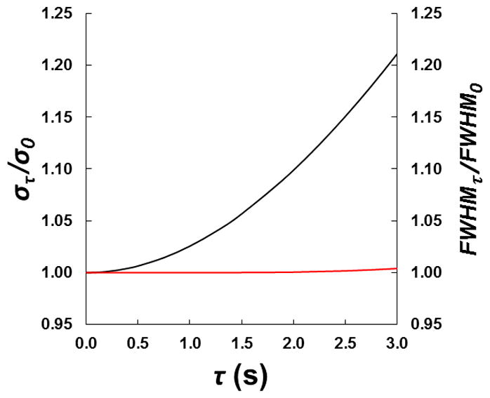
Influence of peak asymmetry on peak variance and half width for a series on exponentially modified Gaussians simulated using σ = 0.75 s, τ = 0.001 to 3 s, α_5% = 1.00 to 7.6. Each Gaussian signal was convolved with a 15 s wide injection plug. Peak variances were calculated using the method of moments, half width measurements were made on each profile and each was normalized to the values obtained from the untailed Gaussian injection. The black trace shows the strong influence of peak tailing on the calculated band variance. The red trace highlights the rather small influence of peak tailing on the bands width at half height.

3. Instrumentation and chromatographic conditions

3.1 Chemicals

Methyl, ethyl, and n-propyl esters of p-hydroxybenzoate (parabens, notated here after as PB1, PB2, and PB3, respectively) and uracil were purchased from Sigma-Aldrich (St. Louis, MO). Standard solutions for parabens were made by dissolving each individually in acetonitrile. Uracil stocks were made in deionized water. Water was from a Millipore Milli-Q Synthesis A10 water purification system (Billerica, MA) and used without further treatment. Acetonitrile (LC/MS Optima grade), isopropanol (HPLC grade), acetone (HPLC grade) and phosphoric acid (HPLC grade) were from Fisher Scientific (Fair Lawn, NJ)

3.2 Instrumentation

Figure 4 shows a simple schematic for the instrumentation used. Waters 1.7 μm d_p Acquity BEH C18 particles (Millford, MA) were packed in-house into 150 μm ID × 360 μm OD fused-silica capillaries from Polymicro Technologies (Phoenix, AZ). Column length was 5.5 cm. The remainder of the column was packed with 8 μm solid silica spheres (Thermo). To determine the extra column time a nominally identical fused-silica capillary was packed with 8 μm solid silica spheres. We refer to this column as the e-column. For complete details related to column preparation see section SI1. The columns packed with stationary phase and 8 μm silica spheres (A) and the e-column (B) were connected directly to a 6-port Cheminert injection valve (C72-6676EH, VICI Valco, Houston, TX) using 1/16″ OD × 0.015″ ID PEEK sleeves (IDEX-Health and Science, Oak Harbor, WA). The additional 3.9 cm segment of each column allowed the unheated, room temperature segment of capillary (2.4 cm) located within the injection valve not to adversely influence the solute retention. In addition 1.5 cm of the capillary served as a mobile phase pre-heater. A 75 cm × 75 μm ID nanoViper capillary (volume = 3.3 μL, Thermo) was used as the sample loop. An Ultimate 3000 RSLCnano high pressure gradient pump (NCP-3200, Thermo, Germering, Germany) was used to deliver mobile phase. Detection was achieved using a Waters Acquity TUV detector equipped with a 10 nL flow cell (Waters) set to 254 nm. The column outlet and flow cell were connected by a 30 cm × 25 μm ID fused-silica detection capillary (Polymicro). Data acquisition and export were achieved by connecting the Acquity TUV analog output to an Agilent 1200 UIB (G1390B, Agilent Technologies, Waldbronn, Germany) and Agilent OpenLab ChemStation CDS software (rev. C01.06). Valve actuation was controlled by a National Instruments USB-6008 DAQ and a simple LabVIEW routine written in-house (rev. 2014, National Instruments, Austin, TX). Column temperature was controlled using a simple homemade resistive heating assembly previously described [28, 29]. Further details regarding instrument configuration and control are provided in the Supporting Information.

Figure 4.

Diagram for the instrumentation used in this work. Two-segment capillary columns (A) consisting of non-interacting silica spheres and stationary phase were attached directly to the injection valve and placed inside a resistively heated insulated enclosure. To accurately determine the extra-column contributions to t₀ injections were made into a so-called e-column (B). The e-column consisted of all portions of the two-segment column except the stationary phase.

3.3 Chromatographic conditions

Precise details related to the preparation of eluents and sample solutions used in this study are critical to interpretation of results. As a result all samples and eluents were prepared gravimetrically in batches large enough to minimize irregularities in sample preparation and absolute mobile phase composition. Mobile phase was prepared by mixing acetonitrile and 10.0 mM H₃PO₄ in water at 5.0, 10.0, and 20.0% (wt%). The 5.0 and 20.0% acetonitrile mobile phases were made in 1.000 kg batches; the 10.0% solvent was prepared at the 0.500 kg scale. Mobile phase was degassed and filtered using 0.45 μm nylon membrane filters (Millipore) prior to use.

Paraben retention studies used 50 nL timed injections of 250 μM uracil, PB1, PB2, PB3 samples made in each mobile phase. Care was taken to maximize peak height by injecting the highest concentration sample without mass overloading the column. Stock solutions employed for retention studies were made at 200 mM in acetonitrile. Spikes, 125 μL, from each stock were made into 100.0 g volumes of premixed mobile phase to achieve desired solute concentration. For retention studies, differences between sample and mobile phase composition were kept less than 0.5%. This small composition difference was due to the additional acetonitrile present in the sample, from the three 125 μL paraben spikes.

Solvent-based focusing studies used large-volume, timed injections corresponding to 500, 1000, 1500, and 2000 nL. Samples were made using 100.0 g portions of the appropriate premixed mobile phase described above. Paraben concentrations were 10 μM each. Samples were prepared from 50 mM stock solutions made in acetonitrile (20 μL spikes). Thus, differences between sample and eluent composition were less than 0.1%.

The premixed mobile phase for retention and injection volume studies, 80:20 10.0 mM H₃PO₄/acetonitrile (wt%), was used as both solvent A and solvent B in the Ultimate 3000 pump. The flow rate was 4.00 μL/min with eluent composition set to 50:50 channel A/B. Column temperature was maintained at 60.0 ± 0.1 °C. All retention studies used samples whose composition was nominally identical to the mobile phase and retention measurements were made with n = 4. Focusing studies were performed in duplicate and used samples made in 95:5, 90:10, and 80:20 10 mM H₃PO₄/acetonitrile (wt%) with mobile phase composition maintained at 80:20 10 mM H₃PO₄/acetonitrile (wt%).

4. Results and discussion

4.1 Accurate determination of solute retention factors

To assess the validity of each focusing model we need accurate retention factors. Mobile phase composition and solutes were selected based on our experience to provide a range of k′ values that would be a good test for the models. Table 1 shows the values of k′ determined from solute retention time at the peak maxima for three mobile phase compositions (80.0:20.0, 90.0:10.0, 95.0:5.0 (wt%)) at 60.0 °C for the three solutes PB1, PB2, PB3. PB3 was omitted from the 5.0% acetonitrile sample due to excessive retention. Retention factors were calculated using Eq. S1 with n = 4. Retention factors were also calculated based on first central moments for uracil and each paraben (see Section SI4). No significant difference in focusing results were obtained using either method.

Table 1.

Experimentally determined retention factors for methylparaben, ethylparaben and propylparaben.

φ	0.20		0.10		0.05
Solute	k′	σk	k′	σk′	k′	σk
PB1	2.06	0.017	7.02	0.019	15.89	0.04
PB2	4.62	0.04	19.62	0.05	50.28	0.13
PB3	10.82	0.08	57.6	0.2	-	-

We note here that evaluation of the models requires accurate measurement of the extent of focusing. This means that injected bands must not be too well-focused or else the natural bandspreading processes will lead to a peak variance that is much larger than the variance of the injected rectangular width. The range of k₁ and k₂ values shown in Table 1 reflects this. As we are using capillary liquid chromatography, extra-column volume can be a significant fraction of, or even exceed, the column volume. We paid particular attention to determining accurate values of t₀ and solute retention times, t_R (see Supporting Information for details), in order to determine accurate values of k₁ and k₂.

4.2 System performance evaluation

As a check on system performance, we performed two control experiments for which the outcome was reliably predictable. In one, a series of timed injections of uracil were made into a 25 μm ID empty tube. As Fig. S4 shows, a plot of the full-width of the rectangular zones (in time units) vs. the injection time is linear. From the slope we can calculate the volumetric flow rate (Eq. S2). Flow rate calculated from the data in Fig. S4 was 3.977 ± 0.030 μL/minute. In the second control experiment, a sample of PB1, PB2, and PB3 was prepared in the mobile phase (80:20 (wt%) phosphate/acetonitrile). Injections from 250 to 1500 nL gave wide eluted zones. Plots of the full-width of the observed zone in units of time vs. the injection time give a slope of 0.992 ± 0.006 and an intercept of −0.008 ± 0.002 (means and 95% confidence intervals, Fig. S5). Full details for performance evaluation experiments are provided in sections S4 and S5 of the Supporting Information. We can conclude from results of both control experiments that system performance is satisfactory for the current work.

4.3 Quantitative evaluation of solvent-based focusing

4.3.1 Solvent-based on-column focusing examples

We made injections of 10.0% (wt%) acetonitrile containing samples of PB1, PB2, and PB3 with V_inj = 500 to 2000 nL into a column with 20.0% acetonitrile as the mobile phase. Fig. 5 shows two example chromatograms in which a small amount of focusing is expected to occur as the composition of the injected solution is weaker than the mobile phase (the full data set is Fig. SI 6). Injection volumes for the black and blue traces were 500 and 1500 nL. Qualitatively it is clearly apparent from Fig. 5 that the 1500 nL injection leads to a volume overloaded peak for PB1 and PB2. Low-retention solutes, particularly PB1 in this demonstration, are most susceptible to volume overload. Under the conditions evaluated, PB1 and PB2 retention factors in the sample solvent and eluent were k₁ = 7.02 and 19.62 with k₂ = 2.06 and 4.62. These factors do not lead to a Gaussian peak shape for the 1500 nL injection.

Figure 5.

Example chromatograms resulting from 500 nL (black) and 1500 nL (blue) injections of paraben samples made in 90:10 wt% 10 mM H₃PO₄/acetonitrile. In each of the two chromatograms, the peaks correspond (in the order of elution) to PB1, PB2, and PB3; mobile phase consisted of 80:10 wt% 10 mM H₃PO₄/acetonitrile. Negative peaks are caused by the injection solvent’s refractive index being different from that of the mobile phase. For chromatographic conditions see Section 3.3.

Fig. 6 shows the results for the full range of injection volumes for each solute under all focusing conditions evaluated. Panels A, B and C correspond to PB1, PB2, and PB3 in 10.0% (wt%) acetonitrile. Panels D, E, and F show PB1, PB2, and PB3 in 5.0% (wt%) acetonitrile. After correcting the time axis for the injection time so that the fronts of all of the zones for a particular solute overlap it can be seen that the peaks get wider as the injection volume increases from 500 to 2000 nL for all solutes. For comparison a 50 nL injection of 250 μM PB1, PB2, and PB3, 5.0% and 10.0 (wt%) acetonitrile, is shown in each panel as a dashed gray line. The relative effect of the injection width on the peak width, as expected, is smaller for the higher k′ compound PB3 than the others. Peak width for each solute in panels D, E, and F is narrower than its analogous injection in panels A, B, and C, as expected, because of the larger values of k₁ in the 5% acetonitrile sample (see Table 1). Note that the PB1 and PB2 peaks in panels D and E still exhibit some signs of volume overload for the largest injection volumes, however the peak widths for PB3 in panel F are constant, varying between 3.1 and 3.3 s across the injection volume range tested (50 nL to 2000 nL). The lack of volume overload for the PB3 peak demonstrates the analytical effectiveness of focusing, but as described above does not help to establish the validity of a quantitative model.

Figure 6.

Time adjusted chromatograms for 500 (black), 1000 (red), 1500 (blue), and 2000 (purple) nL injections of paraben samples made in 90:10 wt% (A–C) and 95:5 wt% (D–F) 10 mM H₃PO₄/acetonitrile; mobile phase consisted of 80:10 wt% 10 mM H₃PO₄/acetonitrile. Panels A and D correspond to PB1; B and E to PB2, and C and F to PB3. The time axes for each large volume injection were aligned to the leading edge of each injection profile. Analogous 50 nL injections for each solute (- - -) are also provided in each panel. For additional chromatographic conditions see Section 3.4. Complete chromatograms for each injection are provided in Figures S7 and S8.

As described above, for clearly volume overloaded peaks with flat tops the simple FWHM measurements can be used to evaluate focusing accurately. When on-column focusing is significant as for PB2 and PB3 in panels E and F, deconvolution will be used to remove the contribution from on-column and post-column processes allowing us to determine the width of the injection profile. In cases such as the just-described PB3 peaks, volume overload has virtually no effect on peak width so deconvolution cannot reveal its magnitude.

4.3.2 Quantitative comparison of focusing models

Fig. 7 is a plot of the expected benefit from solvent-based preconcentration for three cases as a function of the single variable k₂/k₁. The three cases are (red) focusing and compression (Eq.10), the effect of focusing alone (eq. 11, gray), and the prediction of Mills et al. (introduction, lavender). The latter two are ranges because neither effect can be expressed as a function of k₂/k₁only. Thus, the effect at a given value of k₂/k₁depends on the actual values (magnitude) of each of the two retention factors. For example, k₂/k₁ equals 0.25 for pairs of k₂ and k₁ (1.0, 4.0), (5, 20), and (20, 80). For each of these pairs, Eq. 10 predicts the same extent of preconcentration. However, Eq. 11 predicts that the effect of preconcentration will be 0.40, 0.29, and 0.26, respectively. Thus, at the x-axis value of 0.25, Eq. 11 predicts a focusing effect that depends on the actual values of k′. As a result, the prediction of Eq. 11 when portrayed on a plot with k₂/k₁ as the x-axis is a zone, not a line. The boundaries of the zone are defined by the ranges of k₂ and k₁ used (see Fig. 7 legend). For similar algebraic reasons, the prediction of Mills et al. is also a zone. Of course, the prediction for Eq.10 is a straight line. The general conclusions are that the step-gradient-induced compression, while small when considering peak capacity in gradient elution [16–18, 30] is nonetheless significant when considered from the perspective of sensitivity. In addition, for low values of k₂/k₁, which would be the normal case in practice, the Mills et al. theory predicts dramatically better preconcentration than Eq. 10.

Figure 7.

Simulations for the apparent on-column focusing (t_obs/t_inj) resulting from each model were calculated as a function of k₂/k₁. Retention factors were varied from 1 < k₁ < 500 and 1 < k₂ < 20; t_obs/t_inj was calculated for every combination of k₂/k₁ within this range. The lavender and gray bands represent the range of t_obs/t_inj values obtained when varying the ratio of k₂/k₁ based on the model derived by Mills et al. and Eq. 11, respectively. The red line represents the calculated t_obs/t_inj based on the k₂/k₁ model incorporating the effect of the step gradient. Note that for each of the values of k₁ and k₂ simulated using the k₂/k₁ model only a single value for t_obs/t_inj is obtained regardless of the magnitude of k₁ and k₂, i.e. only the ratio of k₂/k₁ matters; this is not predicted by the other two models. As expected all three models for on-column focusing converge at both corners of the plot where no focusing and large amounts of focusing are present.

With accurate values for k₁ and k₂ for each solute and condition, we can calculate the expected effect from each case as shown in Fig. 8 which, as Fig. 7, shows Eq.10 (red), eq. 11 (black) and Mills et al. (blue). Note that the range of values of k₂/k₁(x–axis) is smaller than in Fig. 7. The observed preconcentration effects are shown as red symbols. Within the zones representing the predictions of Mills et al. and Eq. 11, we have plotted open triangles representing the specific prediction for the actual values of k₂ and k₁ used in the experiment. Several things are clear. (1) The data describe, within experimental error, a straight line. This supports the idea that Eq.10 most adequately predicts the combined effects of focusing and compression. The experimental slope is 0.90 which is significantly different than the predicted slope, 1.0. We discuss this below. (2) The prediction of the oft-cited work by Mills et al. is not at all accurate. We do not believe that there is justification for using this model to estimate the allowable volume injected or the achievable sensitivity enhancement. (3) As Snyder points out [30] the effect of compression is small, but it is by no means negligible as Fig. 8 shows by comparing the black and red points for individual k₂/k₁ combinations.

Figure 8.

Quantitative comparison of on-column focusing models. Experimental data based on deconvoluted injection width measurements and retention factors in Table 1 are plotted as red circles. Data points correspond to replicate injections of: 1000, 1500, 2000, and 1500 and 2000 nL injections of methylparaben made in 90:10 and 95:5 wt% 10 mM H₃PO₄/acetonitrile, 1500, 2000, and 2000 nL injections of ethylparaben in 90:10 and 95:5 wt% 10 mM H₃PO₄/acetonitrile, and 2000 nL injections of propylparaben in 90:10 wt% 10 mM H₃PO₄/acetonitrile. A total of 18 data points are plotted corresponding to 5 different k₂/k₁ ratios (red circles). The solid red line corresponds to the degree of focusing predicted by the k₂/k₁ model and experimental k′ values. Bands calculated based on Eq. 11 and the Mills model for the range of k₁ and k₂ values encompassed by the experimental range (see Table 1) are plotted as gray and lavender bands, respectively. Individual points based on each experimental k₁ and k₂ value are also plotted for these two models and shown as open black and blue triangles.

There are several factors that may contribute to the observed deviation from the very simple model. Among the factors to consider are whether values of k′ at constant temperature are accurate, whether temperature control is adequate, and whether pressure changes alter the picture. We have made extensive efforts to account for the potential influence of these parameters on the results presented in Fig. 8. Sections S2, S3, and S4 of the supplemental information address potential inaccuracies in k′ values. Temperature irregularities on the order of a few degrees, either in the form of viscous heating or local temperature variations in the column heating element could not account for the magnitude of the extra compression observed. The high thermal conductivity of fused silica columns as well as operating them under the moderate linear velocities used here are also not likely to induce viscous heating related changes in k′ [31]. Pressurizing the sample in the loop will reduce its volume and thus reduce the initial zone width. The pump pressurizes the loop contents to 425 bar. Sample volume will be decreased less than 2% under these conditions [32]. Thus, it is unlikely that pressure-based compression of the sample either in the loop or at the head of the column can account for the extra compression.

One factor that may explain the extra compression is the actual solvent composition profile on the column when the mobile phase returns to the column behind the injected volume. Consider the simple case in which the solvent front enters the column as a sharp front but spreads as it proceeds down the column. The spreading may be caused by column mass transport dynamics or it may be caused by depletion of organic modifier in the mobile phase at the solvent front as the amount of adsorbed organic modifier increases to equilibrate with the new, modifier-rich mobile phase. Recall that the on-column compression is caused by the fact that the tail of the solute zone moves faster than the front for a particular time governed by the zone width and the mobile phase velocity. If the tail is exposed to an abrupt change in solvent strength, but the front is exposed to a relatively gradual change, extra compression will occur. Note that the change in solvent strength is still quite steep at the front when considered in relation to gradient elution chromatography. The extra compression for the injected band arises because it takes a longer time for the front of the zone to be exposed to final composition of the mobile phase when the solvent composition changes over some distance/time.

Conclusions

In this work we have evaluated quantitatively the accuracy of a pair of k′-based models designed to predict the effectiveness of on-column focusing in liquid chromatography. We can draw the following conclusions:

1. Quantitative comparisons of models for on-column focusing are best made using metrics based on the peak width at half height for volume overloaded peaks rather than those related to peak height or sensitivity enhancement.

2. The frequently derived k₂/k₁ relationship designed to incorporate focusing due to 1) the higher solute retention in the sample solvent and 2) compression from the resulting step gradient of the higher elution strength mobile phase is currently the best available analytical model to describe the effect.

3. The oft-cited model derived by Mills et al. is incorrect and significantly overestimates the on-column focusing effect. Thus, we feel it should no longer be used to model the effectiveness of on-column focusing.

4. While the k₂/k₁ model is reasonably accurate and significantly better than its alternatives, the model does not account for the additional compression of the injected band resulting from the steep (but not “step”) gradient resulting from the mobile phase passing through the injection band.

This work illustrates the utility of the simple k₂/k₁ relationship for solvent-based on-column focusing. While this model underestimates the magnitude of focusing it is easy to use and accurate enough to be practically useful. Experimental results can be expected to be slightly better than those predicted by the model.

Highlights.

• There are two published models for the extent of on-column focusing in LC.

• Aim of study was to quantitatively evaluate each model experimentally.

• Best model: volume/injected volume is k₂/k₁ (mobile phase/sample liquid)

• Experiment supports k₂/k₁ model with some deviation towards increased focusing.

References

- 1.van Deemter J, Zuiderweg F, Klinkenberg A. Longitudinal diffusion and resistance to mass transfer as causes of nonideality in chromatography. Chem Eng Sci. 1956;5:271–289. [Google Scholar]
- 2.Sternberg JC. Advances in chromatography. Vol. 2. New York, NY: United States; 1966. p. 205. [Google Scholar]
- 3.Prüß A, Kempter C, Gysler J, Jira T. Extracolumn band broadening in capillary liquid chromatography. J Chromatogr A. 2003;1016:129–141. doi: 10.1016/s0021-9673(03)01290-1. [DOI] [PubMed] [Google Scholar]
- 4.Vissers J, Deru A, Ursem M, Chervet J. Optimised injection techniques for micro and capillary liquid chromatography. J Chromatogr A. 1996;746:1–7. [Google Scholar]
- 5.Foster MD, Arnold MA, Nichols JA, Bakalyar SR. Performance of experimental sample injectors for high-performance liquid chromatography microcolumns. J Chromatogr A. 2000;869:231–241. doi: 10.1016/s0021-9673(99)00957-7. [DOI] [PubMed] [Google Scholar]
- 6.Héron S, Tchapla A, Chervet JP. Influence of injection parameters on column performance in nanoscale high-performance liquid chromatography. Chromatographia. 2000;51:495–499. [Google Scholar]
- 7.Claessens HA, Kuyken MAJ. A comparative study of large volume injection techniques for microbore columns in hplc. Chromatographia. 1987;23:331–336. [Google Scholar]
- 8.Bakalyar SR, Phipps C, Spruce B, Olsen K. Choosing sample volume to achieve maximum detection sensitivity and resolution with high-performance liquid chromatography columns of 1.0, 2.1 and 4.6 mm i.D. J Chromatogr A. 1997;762:167–185. doi: 10.1016/s0021-9673(96)00851-5. [DOI] [PubMed] [Google Scholar]
- 9.Huber JFK, Hulsman JARJ, Meijers CAM. Quantitative analysis of trace amounts of estrogenic steroids in pregnancy urine by column liquid-liquid chromatography with ultraviolet detection. J Chromatogr A. 1971;62:79–91. doi: 10.1016/s0021-9673(01)96812-8. [DOI] [PubMed] [Google Scholar]
- 10.Kamperman G, Kraak JC. Simple and fast analysis of adrenaline and noradrenaline in plasma on microbore high-performance liquid chromatography columns using fluorimetric detection. Journal of Chromatography B: Biomedical Sciences and Applications. 1985;337:384–390. doi: 10.1016/0378-4347(85)80051-7. [DOI] [PubMed] [Google Scholar]
- 11.Kraak JC, Smedes F, Meijer JWA. Application of on-column concentration of deproteinized serum to the hplc-determination of anticonvulsants. Chromatographia. 1980;13:673–676. [Google Scholar]
- 12.Buonasera K, D’Orazio G, Fanali S, Dugo P, Mondello L. Separation of organophosphorus pesticides by using nano-liquid chromatography. J Chromatogr A. 2009;1216:3970–3976. doi: 10.1016/j.chroma.2009.03.005. [DOI] [PubMed] [Google Scholar]
- 13.Jandera P, Hájek T, Česla P. Effects of the gradient profile, sample volume and solvent on the separation in very fast gradients, with special attention to the second-dimension gradient in comprehensive two-dimensional liquid chromatography. J Chromatogr A. 2011;1218:1995–2006. doi: 10.1016/j.chroma.2010.10.095. [DOI] [PubMed] [Google Scholar]
- 14.Vivó-Truyols G, van der Wal S, Schoenmakers PJ. Comprehensive study on the optimization of online two-dimensional liquid chromatographic systems considering losses in theoretical peak capacity in first- and second-dimensions: A pareto-optimality approach. Anal Chem. 2010;82:8525–8536. doi: 10.1021/ac101420f. [DOI] [PubMed] [Google Scholar]
- 15.Stoll DR, Talus ES, Harmes DC, Zhang K. Evaluation of detection sensitivity in comprehensive two-dimensional liquid chromatography separations of an active pharmaceutical ingredient and its degradants. Analytical and Bioanalytical Chemistry. 2014 doi: 10.1007/s00216-014-8036-9. [DOI] [PubMed] [Google Scholar]
- 16.Snyder LR. Linear elution adsorption chromatography. J Chromatogr A. 1964;13:415–434. doi: 10.1016/s0021-9673(01)95138-6. [DOI] [PubMed] [Google Scholar]
- 17.Snyder LR. Principles of gradient elution. Chromatographic Reviews. 1965;7:1–51. doi: 10.1016/0009-5907(65)80002-3. [DOI] [PubMed] [Google Scholar]
- 18.Snyder LR, Saunders DL. Optimized solvent programming for separations of complex samples by liquid-solid adsorption chromatography in columns. J Chromatogr Sci. 1969;7:195–208. [Google Scholar]
- 19.Lankelma J, Poppe H. Determination of methotrexate in plasma by on-column concentration and ion-exchange chromatography. J Chromatogr A. 1978;149:587–598. doi: 10.1016/s0021-9673(00)81013-4. [DOI] [PubMed] [Google Scholar]
- 20.Poppe H, Paanakker J, Bronckhorst M. Peak width in solvent-programmed chromatography. J Chromatogr A. 1981;204:77–84. [Google Scholar]
- 21.Hsu S-H, Raglione T, Tomellini SA, Floyd TR, Sagliano N, Jr, Hartwick RA. Zone compressesion effects in high-performance liquid chromatography. J Chromatogr A. 1986;367:293–300. [Google Scholar]
- 22.De Vos J, Desmet G, Eeltink S. A generic approach to post-column refocusing in liquid chromatography. J Chromatogr A. 2014;1360:164–171. doi: 10.1016/j.chroma.2014.07.072. [DOI] [PubMed] [Google Scholar]
- 23.De Vos J, Eeltink S, Desmet G. Peak refocusing using subsequent retentive trapping and strong eluent remobilization in liquid chromatography: A theoretical optimization study. J Chromatogr A. 2015;1381:74–86. doi: 10.1016/j.chroma.2014.12.082. [DOI] [PubMed] [Google Scholar]
- 24.Hilhorst MJ, Somsen GW, de Jong GJ. Sensitivity enhancement in capillary electrochromatography by on-column preconcentration. Chromatographia. 2000;53:190–196. [Google Scholar]
- 25.Mills MJ, Maltas J, John Lough W. Assessment of injection volume limits when using on-column focusing with microbore liquid chromatography. J Chromatogr A. 1997;759:1–11. [Google Scholar]
- 26.Šlais K, Kouřilová D, Krejčí M. Trace analysis by peak compression sampling of a large sample volume on microbore columns in liquid chromatography. J Chromatogr A. 1983;282:363–370. [Google Scholar]
- 27.Wright NA, Villalanti DC, Burke MF. Fourier transform deconvolution of instrument and column band broadening in liquid chromatography. Anal Chem. 1982;54:1735–1738. [Google Scholar]
- 28.Zhang J, Jaquins-Gerstl A, Nesbitt KM, Rutan SC, Michael AC, Weber SG. In vivo monitoring of serotonin in the striatum of freely moving rats with one minute temporal resolution by online microdialysis-capillary high-performance liquid chromatography at elevated temperature and pressure. Anal Chem (Washington, DC, U S) 2013;85:9889–9897. doi: 10.1021/ac4023605. [DOI] [PMC free article] [PubMed] [Google Scholar]
- 29.Zhang J, Liu Y, Jaquins-Gerstl A, Shu Z, Michael AC, Weber SG. Optimization for speed and sensitivity in capillary high performance liquid chromatography. The importance of column diameter in online monitoring of serotonin by microdialysis. J Chromatogr A. 2012;1251:54–62. doi: 10.1016/j.chroma.2012.06.002. [DOI] [PMC free article] [PubMed] [Google Scholar]
- 30.Snyder LR. High-performance gradient elution: The practical application of the linear-solvent-strength model. John Wiley; Hoboken, NJ: 2007. [Google Scholar]
- 31.Verstraeten M, Pursch M, Eckerle P, Luong J, Desmet G. Modelling the thermal behaviour of the low-thermal mass liquid chromatography system. J Chromatogr A. 2011;1218:2252–2263. doi: 10.1016/j.chroma.2011.02.023. [DOI] [PubMed] [Google Scholar]
- 32.Billen J, Broeckhoven K, Liekens A, Choikhet K, Rozing G, Desmet G. Influence of pressure and temperature on the physico-chemical properties of mobile phase mixtures commonly used in high-performance liquid chromatography. J Chromatogr A. 2008;1210:30–44. doi: 10.1016/j.chroma.2008.09.056. [DOI] [PubMed] [Google Scholar]
Associated Data
This section collects any data citations, data availability statements, or supplementary materials included in this article.