High-Frequency Replanning Under Uncertainty Using Parallel Sampling-Based Motion Planning

Abstract

As sampling-based motion planners become faster, they can be re-executed more frequently by a robot during task execution to react to uncertainty in robot motion, obstacle motion, sensing noise, and uncertainty in the robot’s kinematic model. We investigate and analyze high-frequency replanning (HFR), where, during each period, fast sampling-based motion planners are executed in parallel as the robot simultaneously executes the first action of the best motion plan from the previous period. We consider discrete-time systems with stochastic nonlinear (but linearizable) dynamics and observation models with noise drawn from zero mean Gaussian distributions. The objective is to maximize the probability of success (i.e., avoid collision with obstacles and reach the goal) or to minimize path length subject to a lower bound on the probability of success. We show that, as parallel computation power increases, HFR offers asymptotic optimality for these objectives during each period for goal-oriented problems. We then demonstrate the effectiveness of HFR for holonomic and nonholonomic robots including car-like vehicles and steerable medical needles.

I. Introduction

In many robotic tasks such as navigation and manipulation, uncertainty may arise from a variety of real-world sources such as unpredictable robot actuation, sensing errors, errors in modeling robot motion, and unpredictable movement of obstacles in the environment. The cumulative effect of all these sources of uncertainty can be difficult to model and account for in the planning phase before task execution. We leverage the increasingly fast performance of sampling-based motion planners available for certain robots, combined with stochastic modeling, to enable these robots to quickly and effectively respond to uncertainty during task execution.

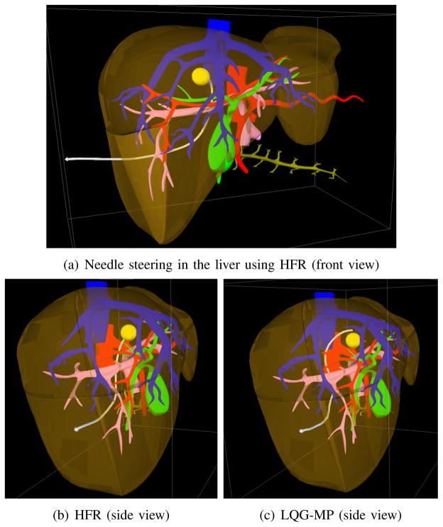
In this paper we consider tasks in which the objective is to maximize the probability of success (i.e., avoid collision with obstacles and reach the goal), or to minimize path length subject a lower bound on the probability of success. We consider holonomic and nonholonomic robots with linear or nonlinear (but linearizable) discrete-time dynamics and with motion and sensing uncertainty that can be modeled as zero-mean Gaussian distributions. We also assume obstacle locations are known or can be sensed. Our approach is applicable to robots for which fast, subsecond sampling-based motion planners are available, including medical steerable needles [30], [31] (see Fig. 1).

Fig. 1.

We apply high frequency replanning (HFR) to medical needle steering in the liver for a biopsy procedure. The objective is to access the tumor (yellow) while avoiding the hepatic arteries (red), hepatic veins (blue), portal veins (pink), and bile ducts (green). To reach the tumor, the needle (white) must pass through several types of tissue: muscle/fat tissue and then liver tissue. The maximum curvature of the needle in the liver is not known a priori and must be estimated during task execution. HFR (a, b) in simulation successfully guided the needle to the tumor by estimating online the needle’s maximum curvature and replanning with high frequency. Using an approach based on preplanning and LQG control (LQG-MP) (c), the needle veered away from the goal and the LQG controller was unable to correct the trajectory.

We investigate and analyze the approach of high frequency replanning (HFR), where the robot executes a motion plan that is updated periodically with high frequency by executing fast sampling-based motion planners in parallel during each period. The replanning computation occurs as the robot is executing the current best plan. If any of the computed plans is better than the plan currently being executed, then the current plan is updated. To select the best plan, we focus on maximizing probability of success or minimizing path length subject a lower bound on the probability of success. We note that for these cost metrics, previous optimal motion planners such as RRT* and related variants [17] cannot be used since the optimal substructure property does not hold. This is because, as shown in Fig. 2, the optimal plan from any configuration to a goal is dependent on the plan chosen to reach that configuration [42]. This substantially complicates the motion planning challenge for the uncertainty-aware cost metrics considered in this paper.

Fig. 2.

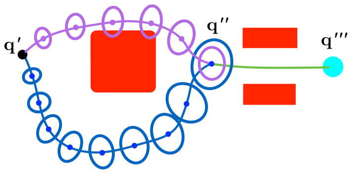
Consider two paths from configuration q′ to a configuration q‴, with ellipsoids representing uncertainty at stages along the paths. RRT* and related asymptotically optimal motion planners assume that the optimal substructure property holds, i.e., if q″ is along the optimal path from q′ to q‴, the subpath from q′ to q″ is itself an optimal path from q′ to q″. While this is true for shortest path problems, optimal substructure does not hold for some uncertainty-aware cost metrics such as maximizing probability of success. Between q′ and q″, the probability of collision for the purple path is larger than the probability of collision for the blue path due to lesser clearance from the obstacles. But the purple plan has lesser estimated uncertainty in state estimation at q″, which will lead to a smaller probability of collision when the robot passes through the narrow passage between q″ and q‴. The lack of optimal substructure when planning in configuration space makes achieving asymptotic optimality more difficult.

HFR combines the benefits of global motion planning with the responsiveness of a controller. By executing multiple sampling-based rapidly-exploring random tree (RRT) [21] motion planners in parallel, under certain reasonable assumptions, HFR will compute at each a period a motion plan that asymptotically approaches the globally optimal plan as computation power (i.e., processor speed and number of cores) increases. For practical problems with finite computational resources, we add a heuristic to HFR to consider newly generated plans as well as the best plan from the prior period adjusted based on the latest sensor measurements and a linear feedback controller. Asymptotic optimality in each period of HFR comes not from generating more configuration samples in a single RRT but rather from generating many independent RRTs (where each RRT terminates when it finds plan and launches a new RRT to begin construction). Another benefit of HFR is that it automatically handles control input bounds since the sampling-based motion planner enforces kinematic and dynamic constraints during plan generation. HFR only applies to goal-oriented problems that do not require returning to previously explored regions of the state space for information gathering, and hence does not address the general POMDP problem [20].

This paper makes three main contributions. First, we show that generating multiple RRTs and selecting the one that optimizes the chosen metric is asymptotically optimal at each period under reasonable assumptions. Asymptotic optimality is important for many applications that require high quality solutions, and gives the user confidence that increasing the computational hardware applied to the problem will result in better and better solutions that improve toward optimality. Second, we present an approach for handling uncertainty by using high-frequency replanning that considers the impact of future uncertainty and uses a heuristic to efficiently adjust the prior best plan based on the latest sensor measurements. Third, we experimentally show that HFR is effective for many problems with uncertainty in motion, sensing, and kinematic model parameters. Evaluation scenarios include a holonomic disc robot navigating in a dynamic environment with moving obstacles whose motion are not known a priori, a nonholonomic car-like robot maneuvering with uncertainty in motion and sensing, and a nonholonomic steerable medical needle [39] maneuvering through tissues around anatomical obstacles to clinical targets under uncertainty in motion, sensing, and kinematic modeling.

II. Related Work

Motion planning under uncertainty has received considerable attention in recent years. Approaches that blend planning and control by defining a global control policy over the entire environment have been developed using Markov decision processes (MDPs) [2] and partially-observable MDPs (POMDPs) [20]. These approaches are difficult to scale, and computational costs may prohibit their application to robots navigating using non-discrete controls in uncertain, dynamic environments. Sampling-based approaches that consider uncertainty [1], [4], [13], [26], [37] or approaches that compute a locally-optimal trajectory and an associated control policy (in some cases in belief space) [32], [36], [41], [43], [46] are effective for a variety of scenarios. But these methods are currently not suitable for real-time planning in uncertain, dynamic, and changing environments where during task execution the path may need to change substantially, potentially across different homotopic classes. Approaches have also been developed to efficiently estimate the probability of collision of plans (and associated control policies) under Gaussian models of uncertainty [8], [33], [42].

An alternative to precomputing a control policy is to continuously replan to account for changes in the robot state or the environment. Several approaches have been suggested for planning in dynamic environments [14], [19], [34], [45], [48], [49] but they do not explicitly account for robot motion and sensing uncertainty. Majumdar et al. [25] use a pre-defined library of motion primitives, which depending on the application can be effective or restrictive. Our work is also related to model predictive control (MPC) approaches [38], which account for state and control input constraints in an optimal control formulation. HFR can be viewed as a variant of MPC control where the goal is always within the horizon and global optimality is achieved (in an asymptotic sense) at each time step using a sampling-based motion planner. In this regard, Du Toit [8] introduced a new method for planning under uncertainty in dynamic environments by solving a nonconvex optimization problem, although this method for some problems is computationally expensive and suffers from local minima. In contrast, HFR is based on an efficient, global motion planner and takes uncertainty into account, resulting in higher probabilities of successful plan execution.

Asymptotically optimal motion planners such as RRT* and related variants [11], [16], [17], [23] return plans that converge toward optimality for cost functions that satisfy certain criteria. In this paper we focus on cost metrics based on probability of success, for which the optimal substructure property does not hold, e.g., the optimal solution starting from any robot configuration is not independent of the prior history of the plan (see Fig. 2). Consequently, RRT* and related variants cannot guarantee asymptotic optimality for our problem without modification. CC-RRT* [24] utilizes RRT* to generate asymptotically optimal motion plans that satisfy user-defined chance constraints. Each node of the CC-RRT* tree explicitly stores a sequence of states and uncertainty distributions of the prior path that leads to the node, enabling optimal substructure. But unlike our approach, CC-RRT* does not consider sensing uncertainty and hence grows the uncertainty distributions in an open-loop fashion by evolving the stochastic dynamics forward in time. In HFR, we explicitly consider the motion and sensing uncertainty and grow the uncertainty distributions in a closed-loop manner using LQG control and an Extended Kalman Filter.

HFR takes advantage of the fact that the speed and effectiveness of sampling-based planning algorithms [6], [22] has improved substantially over the past decade due to algorithmic improvements and innovations in hardware. One source of speedup has been parallelism, including the use of multiple cores or processors (e.g., [5], [7], [10], [15], [28], [35]) and GPUs (e.g., [3], [29]) to achieve speedups for single-query sampling-based motion planners (e.g., RRT and RRT*). Wedge and Branicky showed that periodically restarting sampling-based tree construction can improve the mean and the variability of the runtime of RRT [47]. Our method extends the OR RRT approach [5], [7] to solve a class of problems with asymptotic optimality rather than solely feasibility. Also, unlike prior approaches that leverage parallelism, we explicitly focus on motion planning problems that involve uncertainty in robot motion and sensing and moving obstacles.

III. Problem Statement

Let q ∈ ⊂ ℝ^l denote the robot state which consists of parameters over which the robot has control, such as the robot’s position, orientation, and velocity. Let x ∈ ⊂ ℝⁿ, n ≥ l, denote the system state which includes the robot state and also relevant parameters that can be sensed, such as obstacle positions and velocities, as well as robot-specific parameters over which the robot does not have direct control, such as robot kinematic parameters (e.g., a steerable needle’s maximum curvature in a particular tissue). Note that the robot’s state q is a subset of the whole system’s state x. We define the initial state of the system as x₀.

We assume that continuous time τ is discretized into periods of equal duration Δ such that the t’th period begins at time τ = tΔ. A motion plan π is then defined by a sequence of discrete control inputs π = {u_t: t = 0, …, T}, where u_t ∈ ⊃ ℝ^m is a control drawn from the space of permissible control inputs. Starting from x₀ and applying a control sequence π with number of steps T, the state of the robot at time τ, where 0 ≤ τ ≤ TΔ, is expressed as x(τ, π). For simplicity, we define x_t = x(τ, π), when τ = tΔ.

The whole system evolves according to a stochastic dynamics model

$${\mathbf{x}}_t=f({\mathbf{x}}_{t-1},{\mathbf{u}}_{t-1},{\mathbf{m}}_t),$$ (1)

where m_t models the cumulative uncertainty, including uncertainty in robot and obstacle motion. We assume m_t is from a Gaussian distribution m_t ~ N(0, M_t) with variance M_t.

During task execution, the robot obtains sensor measurements according to the stochastic observation model

$${\mathbf{z}}_t=h({\mathbf{x}}_t,{\mathbf{n}}_t),$$ (2)

where z_t is the vector of measurements and n_t is noise which is from a Gaussian distribution n_t ~ N(0, N_t) with variance N_t.

In addition, our method also requires as input an estimate of the initial system state x̂₀ with corresponding variance Σ̂₀, a cost function c(π, x) that defines the expected cost of a motion plan π from an initial system state x, the period duration Δ, a set of obstacles that may move over time, and a goal region such that x_t ∈ signifies success at time step t. We consider two optimization objectives:

1. Maximize the probability of success, i.e., the probability of avoiding collision with obstacles and reaching the goal. We define the cost function c(π, x) as the negative of the probability of success estimated for plan π.

2. Minimize path length subject to a lower bound on the probability of success. We define c(π, x) as the length of the nominal plan resulting from executing π if the path satisfies the chance constraint (i.e., a lower bound on the estimated probability of success) and as ∞ if the plan violates the chance constraint.

Our approach aims to compute and execute a control input u_t at each time step based on the chosen optimization objective.

IV. Approach

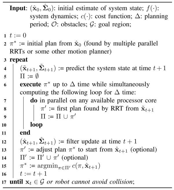
We outline HFR in Algorithm 1. The outer loop of the HFR algorithm (lines 3–17) runs at a high frequency with a period of Δ to address uncertainty in robot motion, obstacle motion, and the robot’s kinematic model. In each period, the bulk of the computation is computing a motion plan. In each period, the robot estimates the system state using a filter, updates the current motion plan with a better motion plan if a better plan is found (as determined by the optimization objective), and then executes the first control input of the current best plan. We assume that except for the inner loop at line 7, other steps are sufficiently fast for real-time computing.

A. Parallel Sampling-Based Replanning

For motion planning, we use a rapidly-exploring random tree (RRT), a well-established sampling-based motion planner [22]. When properly implemented, a RRT provides probabilistic completeness guarantees that, as computational effort increases, a plan will be found if one exists. In HFR, at time step t the RRT is rooted at the system state x̃_t+1, the estimated state of the robot at the next time step (as discussed in Section IV-B). At each iteration of the RRT algorithm, we sample a robot state q_sample ∈ , find its nearest neighbor q_near in the tree, and compute a control u ∈ that grows the tree from q_near toward q_sample using the RRT’s “extend” function, i.e., (q_new, u) = extend(q_near, q_sample) where q_new requires no more than Δ time to reach from q_near [21]. Although motion planning is conducted in the robot’s state space , collision detection may depend on the system state x_t ∈ , especially for cases with moving obstacles. For any q_t ∈ , we can estimate the corresponding x_t ∈ by augmenting the robot state vector at time t to incorporate missing entries from the prior system state and then evolving the vector through the stochastic dynamics function with zero noise. The output of the RRT is a motion plan, π = [u_t+1, u_t+2, …, u_T], that specifies a sequence of control inputs to reach the goal.

Algorithm 1.

HFR Algorithm

During each period, our objective is to compute a motion plan that minimizes the cost function c. Prior asymptotically optimal sampling-based methods (e.g., [17]) are not suitable for cost metrics such as maximizing probability of success for which the optimal substructure property does not hold in configuration space, as shown in Fig. 2.

Our approach to finding an optimal plan is to simultaneously execute a large number of independent RRTs and then select the RRT with the lowest cost plan. By evaluating the cost metric over an entire plan we avoid requiring the optimal substructure property. We refer to lines 7–10 and line 15 as Multiple Parallel RRTs (MPRRT). Specifically, during each period of duration Δ, we execute independent RRTs in parallel on each available processor core. As soon as an RRT finds its first solution, we add the plan to a set Π (line 9) and start executing a new independent RRT on that processor core. As parallel computation power increases, the number of RRT solutions obtained in time Δ rises. We note that any individual RRT, with probability 1, will not compute an optimal plan for a general motion planning problem regardless of how many robot state samples are generated [17]. We show in Sec. V that, for goal-oriented problems with our cost functions and with a finite (although not necessarily known) number of periods, the plan computed by MPRRT will asymptotically approach the optimal plan as computational power increases.

B. Predicting System State for Motion Planning

Since the robot is in motion during replanning and we desire a full period of time Δ for replanning, the computation of the motion plan for period t + 1 must occur during period t. Hence, at the beginning of period t we must predict the system state at the next time step x̃_t+1, which is used to seed the RRTs. Due to uncertainty, the exact state of the system at time (t + 1) Δ cannot be perfectly predicted at time tΔ. To estimate x̃_t+1, we evolve the estimated system state distribution using the system dynamics function (Eq. 1). More formally, we compute x̃_t+1 = f(x̂_t, u), where u is the first control input of the current plan π^* that is being executed. To represent the uncertainty distribution, we truncate the portion of the Gaussian distribution of system state in collision with obstacles [33].

Near the end of each time step t (line 12), we obtain sensor measurement z_t+1 and estimate the system state x̂_t+1 for the next time step. In our implementation, we use an Extended Kalman Filter (EKF). Since the estimated state x̂_t+1 may not equal the state x̃_t+1 that was predicted at the beginning of time step t (line 4), the RRT plans may be rooted at a state that is slightly incorrect. Since HFR plans at high frequency and Δ is small, the deviation in the initial system state in each RRT is expected to be small. We analyze this difference in Sec. V.

C. Optional Heuristic for Adjusting the Prior Best Plan

To improve HFR performance when limited finite computation power is available, we include the prior best motion plan in the set of motion plans considered by the optimization in line 15. However, the prior best plan may have been computed multiple periods earlier, and hence did not consider any of the sensed information from recent periods. For example, the system may be at a significantly different state from the state implied by the prior best motion plan without any adjustments. To incorporate the recently sensed information into the prior best plan in an effective manner, in line 13 of Algorithm 1 we adjust the prior best motion plan to start from x̃_t+1 and adjust the control inputs to the values that would most likely have been performed by a linear quadratic Gaussian (LQG) controller used in conjunction with a Kalman filter.

Specifically, given a prior motion plan π = [ũ_t+1, …, ũ_T] from the predicted system state x̃_t+1, the corresponding nominal trajectory of the RRT plan based on the system dynamics with zero noise is given by Γ = [x̃_t+1, ũ_t+1, …, x̃_T, ũ_T]. We linearize the dynamics and sensing functions around the trajectory Γ and compute an LQG control policy and a Kalman filter [4], [42]. This computation provides a sequence of feedback matrices {L_t} and a sequence of Kalman gains {K_t}. We then compute the maximum likelihood simulated trajectory (MLST) as

$${\mathbf{x}}_{t+2}^{\prime }=f({\mathbf{x}}_{t+1}^{\prime },{\mathbf{L}}_{t+1}({\widehat{\mathbf{x}}}_{t+1}-{\stackrel{\sim }{\mathbf{x}}}_{t+1})+{\stackrel{\sim }{\mathbf{u}}}_{t+1},\mathbf{0})$$ (3)

where x̂_t+1 is updated by the Kalman Filter by assuming each future observation is obtained without sensor noise (maximum likelihood observation [36]),

$${\mathbf{z}}_{t+2}^{\prime }=h({\mathbf{x}}_{t+2}^{\prime },\mathbf{0}).$$ (4)

Starting from ${\mathbf{x}}_{t+1}^{\prime }={\widehat{\mathbf{x}}}_{t+1}$, we compute an adjusted motion plan π′ = [L_t+1(x̂_t+1 − x̃_t+1) + ũ_t+1, …, L_T−1(x̂_T−1 − x̃_T−1) + ũ_T−1, 0] and corresponding $\text{MLST}[{\mathbf{x}}_{t+1}^{\prime },{\mathbf{x}}_{t+2}^{\prime },\dots ,{\mathbf{x}}_T^{\prime }]$. In Algorithm 1, π′ is generated in line 13 and is added into the plan set in line 14 for consideration as the best plan for the next period.

D. Estimating the A Priori Probability of Success of a Plan

Both cost functions introduced in Sec. III require a priori estimation of the probability of success of a motion plan, and this computation needs to be completed very quickly for HFR to operate at high frequency. Under the assumption of Gaussian uncertainty, the a priori distributions of the robot state at each time step over the course of executing a plan can be estimated quickly [4], [33], [42], [46]. These methods typically assume that the robot will execute the plan with an optimal linear feedback controller and use a Kalman Filter variant for state estimation [40], as we assume in our implementation of HFR.

Formally, given a plan π, a nominal trajectory [x̃_t, x̃_t+1, …, x̃_T], and an initial belief N(x̂_t, Σ̂_t), the above methods can be used to estimate a sequence of Gaussian distributions {N(x̃_t′, Σ̃_t′)}, for t ≤ t′ ≤ T. For each time step t′, the mean of the Gaussian distribution is the original nominal system state x̃_t′, while covariance Σ̃_t′ captures the possible deviation from x̃_t′ when the robot is at time step t′ during execution. This sequence of Gaussian distributions captures the distributions of the deviations from the nominal trajectory during the execution of the plan π with the LQG feedback controller. In our implementation, we truncate the Gaussian distributions at each time step to remove portions of the distribution for which collisions would occur and then only propagate the truncated Gaussian distribution to future time steps [33] for computing an accurate, yet conservative, estimate of the probability of success (Fig. 3). More formally, at any time step t′, let us assume the state of the system x_t′ ~ (x̃_t′, Σ̃_t′). Before propagating the distribution to time step t′ + 1, we truncate the Gaussian distribution against obstacles to remove the parts of the distribution that collide with obstacles. The truncated distribution captures the possible states of the system that are collision free at time step t′. Before propagating the uncertainty distribution to the next time step, we fit a Gaussian distribution to the truncated distribution. By propagating the new Gaussian distribution to time step t′ + 1, we only propagate to the next time step states that are collision free. Hence, we properly consider the dependency of uncertainty on previous time steps. Namely, the possible states of the system at time step t′ + 1 should be conditioned on the fact that the system is collision free at time step k, where 0 ≤ k ≤ t′.

Fig. 3.

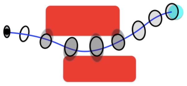
Consider a path from the initial position (black dot) to the goal region (cyan circle). To evaluate the probability of the success of this motion plan, we estimate uncertainty distributions along the motion plan. The probability of collision at each time step is conditioned on the previous stages being collision free. We truncate a Gaussian distribution (gray ellipses) propagated from the previous step against obstacles and then use a Gaussian distribution (black ellipse) to approximate the truncated distribution. We then propagate the new Gaussian distribution (black ellipse) to the next time step.

Using the approach above for estimating the a priori probability of success of a candidate plan, we have the tools necessary to evaluate both of the cost functions c in Sec. III.

V. Analysis

Our analysis of HFR applies to goal-oriented problems: we require the optimal plan π^* to have the property that state ${\mathbf{x}}_t^{\ast }$ along the plan π^* is closer (based on the distance metric used by the RRT) to the state ${\mathbf{x}}_{t-1}^{\ast }$ than to any state ${\mathbf{x}}_{t^{\prime }}^{\ast }$ where t′ < t − 1. For goal-oriented problems, the robot will never return close (i.e., reachable in Δ time) to a previously explored state. There are problems where the optimal solution might not satisfy the requirement above of a goal-oriented problem. For instance, in active information gathering problems, the optimal path may revisit previously explored states. HFR cannot provide any guarantees on performance for problems that are not goal-oriented problems.

We first analyze MPRRT, our approach for executing multiple RRTs in each planning period Δ as described in Sec. IV-A. Our analysis applies to holonomic and nonholonomic robots. We show that for a goal-oriented problem in which a plan is represented by control inputs over a finite number of periods, for the cost functions considered in this paper the plan returned by MPRRT asymptotically converges toward the optimal plan π^* with probability 1.

We then analyze HFR in comparison to following a precomputed plan with an associated closed-form linear control policy (e.g., an LQG controller). We show that, as computational power increases, at each time step t the method will select a control input u_t that is equal or better than a control input generated by a linear feedback controller with respect to the cost metrics considered in this paper, which involve probability of success.

A. Asymptotic Optimality of MPRRT

We first show this MPRRT is asymptotically optimal for goal-oriented problems. To simplify notation we present the analysis assuming = , although the results can be extended to the case where these spaces are distinct by applying the analysis below solely to the elements in . We call a plan α-collision free if all states along the plan are a distance of at least α from any obstacle. We consider cost functions for which α for an optimal solution is non-zero, which is reasonable for safe motion planning under uncertainty and is satisfied by the cost functions considered in this paper.

Given starting state x₀ and two feasible plans π₁ and π₂, we define the distance between π₁ and π₂ as ||π₁ − π₂|| = max_ζ∈[0,1]||x(ζT₁Δ, π₁) − x(ζT₂Δ, π₂)||, where T₁ is the number of periods of π₁ and T₂ is the number of periods of π₂.

Assumption A

The cost function c is Lipschitz continuous, i.e., there exists some constant K such that starting from x₀, for any two feasible sequence of controls π₁ and π₂, ||c(π₁, x₀) − c(π₂, x₀)|| ≤ K||π₁ − π₂||.

Assumption A expresses that two plans that are close to each other have similar cost.

Assumption B

The discrete-time dynamics function x_t+1 = f(x_t, u_t, 0)

• is locally Lipschitz continuous, and

• can be approximated as x_t+1 = x_t + Δẋ_t for a sufficiently small duration Δ.

The second point of assumption B assumes that the system dynamics can be locally approximated as linear, which is also assumed by many previous methods (e.g., [33], [42]) for motion planning under uncertainty.

Given a plan π = [u₀, u₁, …, u_T] and x₀, we define Γ = [x₀, u₀, x₁, u₁, …, x_T, u_T] as the nominal trajectory when executing π from x₀ with zero process noise.

Assumption C

There exists an optimal plan such that the corresponding optimal nominal trajectory can be expressed in a discrete form as ${\mathrm{\Gamma }}^{\ast }=[{\mathbf{x}}_0^{\ast },{\mathbf{u}}_0^{\ast },\dots ,{\mathbf{x}}_T^{\ast },{\mathbf{u}}_T^{\ast }]$ for some finite T, where ${\mathbf{u}}_T^{\ast }=0$, and there exists a constant α ∈ R⁺ such that Γ^* is α-collision free.

Assumption C requires that the optimal trajectory Γ^* has a finite (but possibly unknown) number of steps and is some nonzero distance away from obstacles. Assumption C is satisfied for the optimization objectives considered in this paper.

Using Assumption B, we show the following lemma.

Lemma V.1

$\forall ({\mathbf{x}}_t^{\ast },{\mathbf{u}}_t^{\ast },{\mathbf{x}}_{t+1}^{\ast })$, where ${\mathbf{x}}_{t+1}^{\ast }=f({\mathbf{x}}_t^{\ast },{\mathbf{u}}_t^{\ast },\mathbf{0})$, there exists constants δ and L such that, for any (x_t, u_t), if $\Vert {\mathbf{x}}_t-{\mathbf{x}}_t^{\ast }\Vert \le \delta$ and $\Vert {\mathbf{u}}_t-{\mathbf{u}}_t^{\ast }\Vert \le \delta$, then

• $\Vert f({\mathbf{x}}_t,{\mathbf{u}}_t,\mathbf{0})-f({\mathbf{x}}_t^{\ast },{\mathbf{u}}_t^{\ast },\mathbf{0})\Vert \le 2L\delta$, i.e., $\Vert {\mathbf{x}}_{t+1}-{\mathbf{x}}_{t+1}^{\ast }\Vert \le 2L\delta$, and

• $\Vert {\mathbf{x}}_{t^{\prime }}-{\mathbf{x}}_{t^{\prime }}^{\ast }\Vert \le 2L\delta$ for any time t′ ∈ (t, t + 1).

The first part of lemma V.1 is derived from the first part of assumption B. The second part of assumption B implies the second part of lemma V.1.

Inspired by the ideas in [18] and based on lemma V.1, we can build “balls” along the optimal trajectory Γ^*. Given any ε ∈ (0, min(α, δ)), for any ( ${\mathbf{x}}_t^{\ast },{\mathbf{u}}_t^{\ast }$), we define ε, t-ball $B_{{\mathbf{x}}_t^{\ast }}$ as $\Vert {\mathbf{x}}_t-{\mathbf{x}}_t^{\ast }\Vert \le \frac{\epsilon }{{(2L)}^{T-t}}$ centered at ${\mathbf{x}}_t^{\ast }$ and we define ε, t-ball $B_{{\mathbf{u}}_t^{\ast }}$ as $\Vert {\mathbf{u}}_t-{\mathbf{u}}_t^{\ast }\Vert \le \frac{\epsilon }{{(2L)}^{T-t}}$ centered at ${\mathbf{u}}_t^{\ast }$. At time step t, if the robot is at a state within $B_{{\mathbf{x}}_t^{\ast }}$ and executes a control input within $B_{{\mathbf{u}}_t^{\ast }}$, then based on lemma V.1 the robot will reach a state within $B_{{\mathbf{x}}_{t+1}^{\ast }}$. Based on the latter result of lemma V.1 and the choice of ε, any state between time t and t+1 belongs to a bounded space centered at the corresponding state on the segment ( ${\mathbf{x}}_t^{\ast },{\mathbf{x}}_{t+1}^{\ast }$), and hence is collision free as well. Given a path π that has the same number of periods as the optimal path π^*, we call path π an ε, t-ball path if and only if for any (x_t, u_t) on π, ${\mathbf{x}}_t\in B_{{\mathbf{x}}_t^{\ast }}$ and ${\mathbf{u}}_t\in B_{{\mathbf{u}}_t^{\ast }}$.

We consider the RRT algorithm as described in Sec. IV-A, where the RRT terminates as soon as the first path is found. We require that the sampling strategy cover the state space and that the RRT node expansion/steering function adequately covers the control input space as described below.

Assumption D

Consider a robot at state x for which there exists a ball of controls B_U of nonzero volume that can feasibly move the robot in Δ time to a state inside a ball B_x′ with nonzero volume centered at x′. The extend(x, x″) function in RRT is implemented such that there is a non-zero probability that, for a sample x″ sampled from B_x′, the extend function returns a control u ∈ B_U to a next state x‴ ∈ B_x′.

We note that many commonly used implementations of the RRT extend function satisfy the assumption above, such as the simple strategy of randomly generating several controls and selecting the control that moves the robot closest to the sampled state.

Theorem V.2

(MPRRT is asymptotically optimal) Let π_i denote the best plan found after i RRTs have returned solutions. Given the assumptions above and assuming the problem is goal-oriented and admits a feasible solution, as the number of independent RRT plans generated in MPRRT increases, the best plan almost surely converges to the optimal plan π^*, i.e., P(lim_i→∞||c(π_i, x₀) − c(π^*, x₀)|| = 0) = 1.

Proof

Without loss of generality, we assume ε is sufficiently small (ε < min(α, δ)). We build ε, t-balls along Γ^* for any ε. Consider a sequence of events that can generate a ε, t-ball path. In a single RRT tree, we start from the initial state ${\mathbf{x}}_0^{\ast }$. From Assumption D, we know there is non-zero probability that RRT can generate a control in $B_{{\mathbf{u}}_0^{\ast }}$ to extend to a new state in $B_{{\mathbf{x}}_1^{\ast }}$. RRT then samples a state. The probability of the newly sampled state ending in $B_{{\mathbf{x}}_1^{\ast }}$ is non-zero since $B_{{\mathbf{x}}_1^{\ast }}$ has non-zero volume. Because of the goal-oriented assumption, the sampled state is closest to the newly generated state in $B_{{\mathbf{x}}_1^{\ast }}$ and the extend function extends the tree from the state in $B_{{\mathbf{x}}_1^{\ast }}$ to the sampled state. Again, based on Assumption D, there is non-zero probability that RRT can generate a control in $B_{{\mathbf{u}}_1^{\ast }}$ to extend to a new state in $B_{{\mathbf{x}}_2^{\ast }}$. The process keeps going until the final state ends up in $B_{{\mathbf{x}}_T^{\ast }}$. Since we assume the optimal plan has finite steps and in each step we have non-zero probability to generate a control that leads to a new state ending inside the next ε, t ball centered around the corresponding state of the optimal plan, the probability of generating an ε, t-ball path by one execution of RRT is nonzero. Note that an ε, t-ball path must be an ε-close path, i.e., for any (x_t, u_t) on π, $\Vert {\mathbf{x}}_t-{\mathbf{x}}_t^{\ast }\Vert \le \epsilon$ and $\Vert {\mathbf{u}}_t-{\mathbf{u}}_t^{\ast }\Vert \le \epsilon$. Thus the probability of generating an ε-close path is non-zero as well, which we express as P_ε ∈ R⁺. Hence we have $P(\Vert {\pi }_i-{\pi }^{\ast }\Vert >\epsilon )={(1-P_{\epsilon })}^i={\overline{P}}_{\epsilon }^i$. Thus, ${\sum }_{i}P(\Vert {\pi }_i-{\pi }^{\ast }\Vert >\epsilon )={\sum }_i{\overline{P}}_{\epsilon }^i\le \frac{1}{1-{\overline{P}}_{\epsilon }}<\infty$. Based on a Borel-Cantelli argument [12], we have P(lim_i→∞||π_i − π*|| = 0) = 1. Since the cost function is Lipschitz continuous based on assumption A, P(lim_i→∞||c(π_i, x₀)−c(π*, x₀)|| = 0) = 1.

Although each independent RRT is not asymptotically optimal as the number of configuration samples rises [17], we have shown that when the above assumptions hold, as the number of feasible plans from independent RRTs approaches infinity, the best plan returned by MPRRT will almost surely converge to an optimal plan. However, as in RRT* and related methods, MPRRT will not exactly generate the optimal plan since optimal plans have zero-measure volume [17].

B. Analysis of HFR

We analyze HFR assuming replanning from scratch each period (i.e., without using the MLST heuristic). Continuing with the results of Sec. V-A, we assume computation power approaches infinity in lines 7–10 in HFR and assume Δ is small such that the difference between x̃_t+1 and x̂_t+1 is small.

We define ${\pi }_{{\widehat{\mathbf{x}}}_t}^{\ast }$ as the optimal plan that starts from x̂_t. The plan ${\pi }_{{\widehat{\mathbf{x}}}_t}^{\ast }$ has a finite number of periods T and is α_t-collision free where α_t ∈ R⁺. Let η_t be the shortest distance between the system state at the last period and the goal region . Let ${\epsilon }_t=min(\frac{{\alpha }_t}{2},\delta ,{\eta }_t)$ and build ε_t, t-balls along ${\pi }_{{\widehat{\mathbf{x}}}_t}^{\ast }$, resulting in a ball centered at x̂_t with radius $r_t=\frac{{\epsilon }_t}{{(2L)}^T}$. We define π_x̃tas a plan starting at x̃_t with the sequence of controls in ${\pi }_{{\widehat{\mathbf{x}}}_t}^{\ast }$.

We first generalize theorem V.2 as follows.

Theorem V.3

For any plan π′, if it has a finite number of periods and there exists an α ∈ R⁺ such that π′ is an α-collision free plan, then MPRRT will generate a plan that almost surely converges to π′.

The proof for theorem V.3 is similar to that of theorem V.2 and requires defining a sequence {π_i}_i∈N⁺ of plans where π_i is a plan that is the closest to π′ after i RRT plans are generated. Using theorem V.3, properly accounting for collisions, and assuming the cost of the paths are computed after estimating the state (line 15 of HFR), we can show that if ||x̂_t − x̃_t|| ≤ r_t, asymptotic optimality is retained in each period. We note that the threshold r_t may be small but does not need to be zero.

Theorem V.4

Assume Δ is small such that at any time step t in HFR, ||x̂_t − x̃_t|| ≤ r_t holds. Let π* be the plan with least cost returned by HFR and let π_c be any possible plan (a sequence of controls) that would have been executed by a linear feedback controller. Then, at time step t, executing the first control of π^* is better than or at least equal to executing the first control of π_c with respect to the cost metric.

We can prove theorem V.4 by computing the control input u_t that would be executed at time step t using the closed form formula for a linear controller. We define π_c as the best plan that could be executed with the first control input being u_t. Since the optimal plan π* computed by HFR satisfies c(π^*, x̂_t) ≤ c(π_c, x̂_t), HFR is at least as good as a linear controller with respect to the cost metric at each time step t.

Theorem V.4 holds only as computation power increases. For practical problems where computation power is limited, we optionally add the MLST of the prior best plan (lines 13 and 14) to the set of considered plans. If MPRRT does not find a better plan than the MLST during the planning period, then by the construction of the MLST, the robot will execute a control that is the same as the control that would have been executed if an LQG controller was applied.

VI. Experiments

We apply HFR to three robots: (1) a holonomic robot, (2) a nonholonomic car-like robot, and (3) a nonholonomic steerable medical needle. We tested our C++ implementation on a PC with two 2.00 GHz Intel (R) Xeon (R) processors (12 processor cores total).

A. Holonomic Robot with Two Moving Obstacles

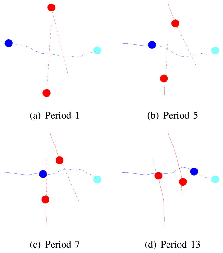
We consider a scenario, based on Du Toit et al. [8], [9], where a holonomic robot moves to a goal state while two dynamic moving obstacles cross the space between the robot and the goal (see Fig. 4). Following the setup of Du Toit [8] (Sec. 4.1.4.3), we define the robot state by its position and velocity, q_t = (x, y, v_x, v_y). The heading of the robot θ can be computed from v_x and v_y. The control input u is a 2-D vector that encodes change in velocity. We define the obstacle’s state as o = (o_x, o_y, o_vx, o_vy), which consists of the 2-D position and the 2-D velocity. Then, the system state at any time step t is defined as x = (q, o¹, o²) where q is the state of the robot and oⁱ is the state of the i’th obstacle (i ∈ {1, 2}). The robot does not have direct control on the parameters oⁱ. The dynamics of the robot are governed by

Fig. 4.

HFR applied to a holonomic robot with two moving obstacles. The robot (dark blue) is moving to a goal (sky blue) and must avoid two moving obstacles (red) that travel roughly up-down and cross the robot’s intended path. In each period of execution shown, the solid lines represent past motions and the dashed lines represent planned motions. Until period 5, the robot was planning to react to the upper moving obstacle by passing from below. Between periods 5 and 7, the robot found a new, better plan passing the upper moving obstacle from above. The robot avoided local minima by successfully finding a new, better plan in a different homotopic class.

$${\mathbf{q}}_t={\mathbf{Aq}}_{t-1}+{\mathbf{Bu}}_{t-1}+{\mathbf{Fw}}_{t-1}$$ (5)

where

$$\mathbf{A}=\left[\begin{array}{cccc}1& 0& \mathrm{\Delta }& 0\\ 0& 1& 0& \mathrm{\Delta }\\ 0& 0& 1& 0\\ 0& 0& 0& 1\end{array}\right],\mathbf{B}=\left[\begin{array}{cc}0& 0\\ 0& 0\\ 1& 0\\ 0& 1\end{array}\right],\text{and}\mathbf{F}=\left[\begin{array}{cc}0& 0\\ 0& 0\\ 1& 0\\ 0& 1\end{array}\right].$$

The 4-D noise term w_t−1 ~ (0, W), where W = 0.01 × I. We set Δ to 0.5 seconds. We assume the system can receive observations of the robot’s position and the obstacles’ positions, which gives the sensing model

$$h(\mathbf{x},\mathbf{n})={[x,y,o_x^1,o_y^1,o_x^2,o_y^2]}^{\top }+\mathbf{n},$$ (6)

where the 6-D sensing vector consists of the robot’s position and the two obstacles’ positions, corrupted by a 6-D noise vector n ~ (0, N), where N = 0.01 × I.

Following Du Toit et al. [8], [9], we set the robot’s initial pose q₀ = (x, y, v cos θ, v sin θ) by setting x = 0, sampling y uniformly from [−2, 2], sampling θ uniformly from [−22.5°, 22.5°] (where θ = 0 represents the direction of horizontal to the right), and setting the initial velocity v to 1.2. The goal is at (12, 0), so the robot moves roughly to the right. For both obstacles, the initial x position is uniformly sampled from [4, 6]. The initial y positions for the two obstacles are fixed to 6 and −6. The initial heading of the top obstacle is uniformly sampled from [−120°, −75°] while the initial heading of the bottom obstacle is uniformly sampled from [75°, 120°]. The initial velocity for both obstacles is set to 1. Hence, the crossing obstacles start from random locations near the top and bottom of the environment and move at random headings roughly up/down. The obstacles move based on the dynamics model in equation 5 with the control inputs set to 0:

$${\mathbf{o}}_t={\mathbf{Ao}}_{t-1}+{\mathbf{Fw}}_{t-1}.$$ (7)

Using this scenario, we compare HFR to Partially Closed-Loop Receding Horizon Control (PCLRHC) [9], which is a receding horizon control approach specifically designed for dynamic, uncertain environments. As in [8], for given motion plans of the robot and the moving obstacles, we use the EKF with the maximum likelihood observation assumption to propagate the uncertainty modelled as a Gaussian distribution from the first step of the plan to the end of the plan. Identical to the setup in [8], we use a cost function related to shortest path subject to a chance constraint of less than 1% probability of failure at each time step. Control magnitude is constrained to be less than 1 at each step. At each time step, each velocity component is subject to chance constraints of P (v_x > 2) ≤ 1% and P (v_x < −2) ≤ 1%, and similarly for v_y.

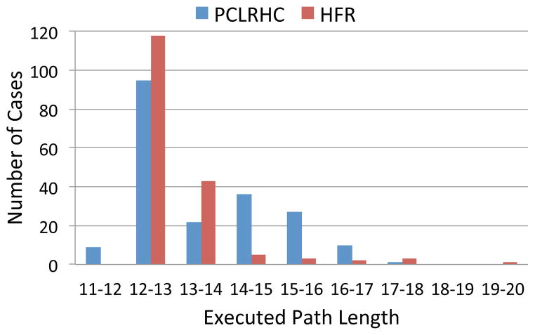
We randomly simulated 200 executions using HFR, and in 176 cases the robot reached the goal while satisfying the constraints, implying an 88% success rate. We verified that the chance constraint of a 1% maximum failure rate at each period was achieved. We show a simulated run of HFR in Fig. 4. We compare the path lengths achieved by HFR to the path lengths achieved by PCLRHC [8] in Fig. 5. HFR more regularly achieves lower path lengths, even though PCLRHC in some cases stops short of the goal when the local optimization criteria are satisfied. HFR achieves a lower average path length because, unlike PCLRHC, HFR automatically explores multiple homotopic classes and is not sensitive to local minima.

Fig. 5.

Histogram of executed path lengths for HFR and for PCLRHC [8]. Note that the length of the shortest path that connects the start position and the goal position is at least 12. PCLRHC occasionally returns values that are less than 12, which is likely due to the robot not exactly reaching the goal. HFR achieves a lower average path length because, unlike PCLRHC, HFR is not sensitive to local minima.

B. Nonholonomic Car-like Robot

We also apply HFR to a nonholonomic car-like robot with 2nd-order dynamics in a 2-D environment with obstacles. The state of the robot q = (x, y, θ, v) consists of the robot’s 2-D position (x, y), its orientation θ, and its speed v. Here the system state x and the robot state q are the same. Its control input u = (α, ϕ) is a 2-D vector consisting of an acceleration α and the steering wheel angle ϕ, corrupted with noise m = (α̃, ϕ̃) ~ (0, M). This gives the nonlinear dynamics model

$$f[\mathbf{x},\mathbf{u},\mathbf{m}]=\left[\begin{array}{c}x+\tau vcos\theta \\ y+\tau vsin\theta \\ \theta +\tau vtan(\varphi +\stackrel{\sim }{\varphi })/d\\ v+\tau (\alpha +\stackrel{\sim }{\alpha })\end{array}\right],$$ (8)

where τ is the time step and d is the length of the car. The robot can sense its position and speed, giving us the stochastic sensing model

$$h(\mathbf{x},\mathbf{n})=\left[\begin{array}{c}x\\ y\\ v\end{array}\right]+\mathbf{n},$$ (9)

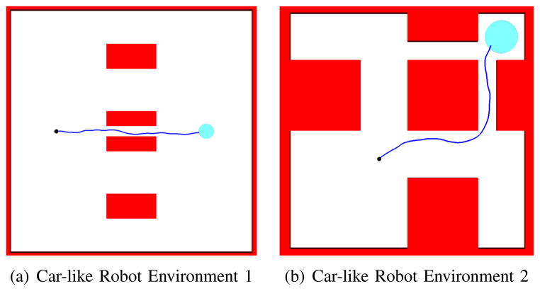
where the 3-D observation vector consists of the robot’s (x, y) position and its velocity v, corrupted by a 3-D sensing noise vector n ~ (0, N). We evaluate HFR for this car-like nonholonomic robot in two environments shown in Fig. 6 to demonstrate HFR’s convergence to optimality and performance with respect to the planning period Δ.

Fig. 6.

We evaluate HFR for a car-like robot in two environments: (a) an environment with a known optimal motion plan, and (b) a more complex planar environment previously used by Patil et al. [33]. The environments include the robot’s initial position (black dots), the goal region (sky blue discs), and obstacles (red rectangles) that divide the environment into several different homotopic classes.

1) Environment with Known Optimal Plan

We applied HFR to the car-like robot in the environment shown in Fig. 6(a) for which the the optimal plan is known. The optimization objective for this scenario is to minimize path length subject to a chance constraint that P (collision free) ≥ 90%. We set M = 0.001 × I and N = 0.0001 × I. With this cost function and this low uncertainty, the optimal plan for the environment in Fig. 6(a) is to move in a straight line from the initial position to the goal region while passing through the middle narrow passage. For this environment, when executed a single time to find only a feasible solution, the RRT is more likely to find a suboptimal solution moving through a wider passage than to find the optimal solution moving through the narrow passage.

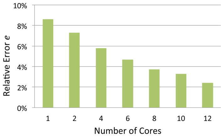
We evaluate the performance of HFR as parallel computation power increases, i.e., as the number of CPU cores increases. For each given number of available cores, we executed HFR 100 times and computed the average path length of all successful executions. We provide HFR 2 seconds to compute an initial plan and we set Δ = 0.5 seconds. We computed the relative error e between the average path length L̄ and the optimal path length L^* as $e=\frac{\overline{L}-L^{\ast }}{L^{\ast }}$. As shown in Fig. 7, the robot using HFR moves along a path that is closer to the globally optimal solution as the number of processor cores increases. The relative error drops to below 3% when the number of CPU cores rises to 12.

Fig. 7.

Convergence to the optimal solution for the car-like robot in environment 1 as the number of processor cores increases.

2) Performance with Respect to Δ

We also applied HFR to a more complex scenario for which the optimal solution cannot be computed analytically. We consider the environment shown in Fig. 6(b) and use the optimization objective of maximizing the probability of success (i.e., reaching the goal while not colliding with obstacles). To model a more realistic car-like robot operating at higher speeds, we also set the process uncertainty to be linearly dependent on the robot’s velocity. Specifically, we set N = 0.005 × I and M = v × 0.001 × I.

Using this scenario, we ran HFR for different values of Δ and measured the probability of success over 100 simulated runs. For comparison, we also ran LQG-MP [42] for the same scenario and computed the probability of success over 100 simulated runs. Both HFR and LQG-MP were allowed 2 seconds for pre-computing plans and selecting the best plan as the initial plan. As shown in Fig. 8, decreasing the value of Δ improves the probability of success for HFR since the predicted start of the robot for planning each period is more accurate and the robot can respond more quickly to uncertainty. This result is consistent with Theorem V.4. Fig. 8 also shows that HFR consistently has a higher probability of success than LQG-MP. We also show an example execution of HFR with Δ = 0.25 in Fig. 6(b).

Fig. 8.

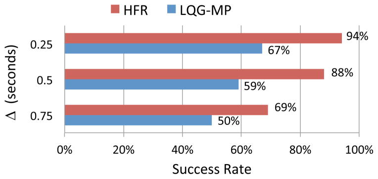
The performance of HFR and LQG-MP for different values of Δ for the car-like robot in environment 2. HFR performs replanning with period Δ, and for LQG-MP Δ is used to determine the time step size of the computed LQG controller.

C. Nonholonomic Steerable Needle

We also apply HFR to a flexible bevel-tip steerable medical needle [39], a type of steerable needle that bends in the direction of the bevel when inserted into soft tissue. By axially rotating the needle, the direction of the bevel can be adjusted, enabling the needle to follow curved trajectories in 3D tissue environments with obstacles. The motion of the steerable needle tip has non-linear dynamics and can be modeled as a nonholonomic robot.

Following the derivation in [44], we describe the state of the needle q by the 4×4 matrix $\mathbf{X}=\left[\begin{array}{cc}\mathbf{R}& \mathbf{p}\\ \mathbf{0}& 1\end{array}\right]$ where R ∈ SO(3) is the rotation matrix and p ∈ ℝ³ is the position of the needle tip. The system state x consists of the robot’s state q and a kinematics parameter κ_max, which represents the maximum curvature of the needle. The curvature of the needle can be varied by applying duty cycled spinning during the needle’s insertion [27]. The control inputs u = [v, w, k]^T ∈ ℝ³ consist of the insertion speed v along the z axis, the twist angular velocity w, and the curvature κ. We describe the dynamics of the needle tip in terms of the instantaneous twist U ∈ se(3) expressed in a local coordinate frame attached to the needle tip: $\mathbf{U}=\left[\begin{array}{cc}[\mathbf{w}]& \mathbf{v}\\ \mathbf{0}& 0\end{array}\right]$, where w = [vκ, 0, w]^T, v = [0, 0, v]^T, and the notation [s] for a vector s ∈ ℝ³ refers to the 3 × 3 skew symmetric cross product matrix. The instantaneous twist U′ encodes the additive motion noise m = [v′, w′]^T ~ (0, M) in a similar way.

Given time step duration Δ, the stochastic discrete-time dynamics of the needle tip is given by the model

$$f(\mathbf{x},\mathbf{u},\mathbf{m})=\left[\begin{array}{c}\mathbf{X}exp(\mathrm{\Delta }(\mathbf{U}+{\mathbf{U}}^{\prime }))\\ {\kappa }_{max}\end{array}\right],$$ (10)

where the control input u cannot directly control κ_max, which is fully determined by the physical properties of the needle and the tissue the needle tip is moving through. Below, we consider two different scenarios: (1) a scenario where κ_max is a priori known, and (2) a scenario where κ_max is not known and needs to be estimated online during needle insertion.

We assume that noisy observations of needle tip pose are obtained my medical imaging or electromagnetic sensing. The noise in the sensing measurement is modeled as n ~ (0, Q). This gives the stochastic measurement model

$$h(\mathbf{x},\mathbf{n})=\mathbf{q}+\mathbf{n}.$$ (11)

The steerable needle has non-linear dynamics, and van den Berg et al. provide details about linearizing the needle dynamics and sensing models for LQG control [44].

1) Artificial Environment Scenario

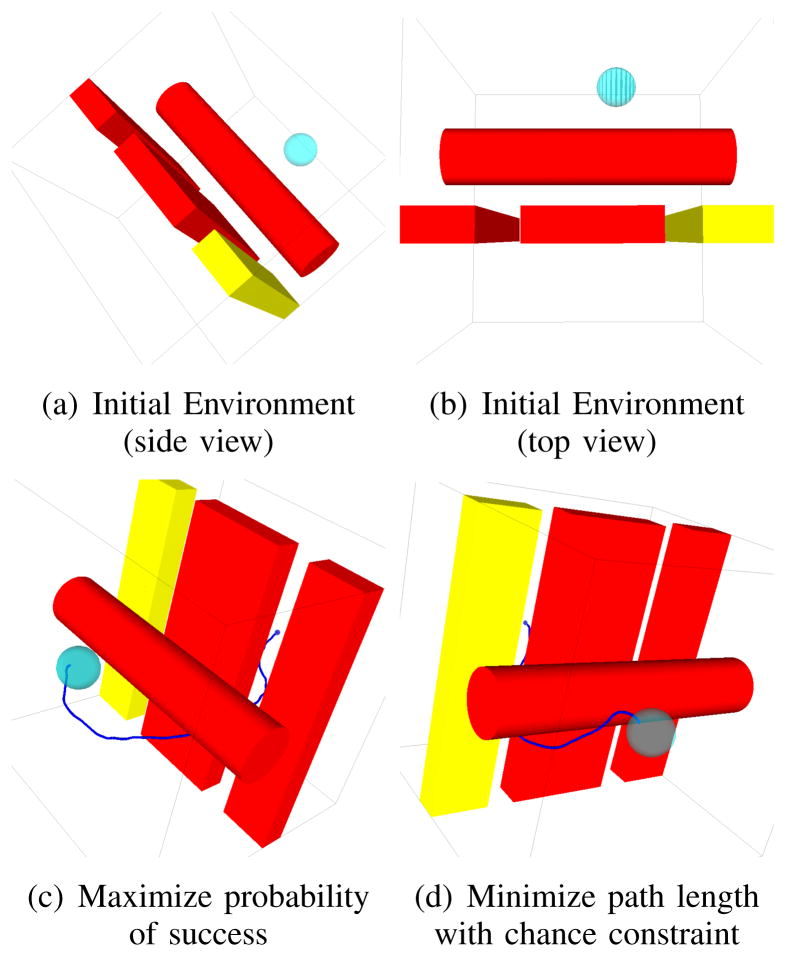
We apply HFR under two optimization objectives: maximizing probability of success and minimizing path length with a chance constraint of P (Collision free) ≥ 80%. We set the needle motion and sensing model parameters to v_max = 1.5 cm/s, w_max = 2π rad/s, Δ = 0.5 s, κ_max = 2 (cm)⁻¹, Q = 0.1 × I, and M = 0.005 × I.

In Fig. 9 we show the environment and a simulated successful run under each of the cost functions. A plan through the passage between red obstacles (i.e., the slightly wider passageway) offers the highest probability of success. A plan next to the yellow obstacle minimizes path length under the given chance constraint.

Fig. 9.

(a) The artificial environment for the steerable needle has two narrow passages in a 10 cm × 10 cm × 10 cm box. The goal region (sky blue sphere) is defined in ℝ³ with radius 0.5 cm. (b) The passage between the two red boxes (1.2 cm) is wider than the passage between the yellow box and the middle red box (1.0 cm). The goal is closer to the narrower passage. (c) For highest probability of success, HFR guided the needle to pass through the wider passage in order to acheive a higher probability of success. (d) For minimizing path length with the defined chance constraint, HFR guided the needle to pass through the passage between the yellow box and the middle red box to acheive a shorter path while still satisfying the chance constraint.

Table I shows that our method outperforms other methods based on LQG control. For each run with LQG-MP [42], we generate 1000 RRT plans, select the best plan using the LQG-MP metric, and then execute an LQG controller along the selected plan. For each run with Preplan+LQG, we generate 1000 RRT plans, select the best plan using a truncated Gaussian approach [33], and then execute an LQG controller along the selected plan. Approximately 5 seconds are required to generate 1000 feasible plans. We ran each method for 100 runs. HFR performed best on both metrics due to its ability to refine plans during execution.

TABLE I.

Comparison of HFR with LQG-MP and Preplan+LQG for the nonhonomic steerable needle

	Highest probability of success (success rate)			Shortest path with chance constraint (Average path length ± STD)
Method:	LQG-MP	Preplan+LQG	HFR	Preplan+LQG	HFR
Performance:	90%	94%	98%	11.64±0.32	11.13±0.59

2) Liver Biopsy Scenario

We consider steering a needle through liver tissue while avoiding critical vasculature. We use the same needle model as before except we assume the maximum curvature of the needle varies by tissue type and is a priori unknown to the robot. For muscle/fat tissue outside the liver, ${\kappa }_{max}^{\text{out}}=5{\text{cm}}^{-1}$, and for the liver tissue, ${\kappa }_{max}^{\text{in}}=4{\text{cm}}^{-1}$. Although the curvature ${\kappa }_{max}^{\text{in}}$ is a priori unknown to the robot, we assume the system can accurately sense the needle tip pose (with Q = 0.0001 × I) to assist in curvature estimation. HFR can easily be integrated with curvature estimation by replanning with the latest estimated maximum curvature at each time step.

Since the curvature κ of the needle is linearly dependent on the proportion β of time spent in duty cycled spinning in one insertion duration [27], we model the relationship between β and κ as $\beta =1-\frac{\kappa }{{\kappa }_{max}}$ where κ_max is the maximum curvature feasible in the tissue. The high level control u = [v, w, κ]^T thus can be transformed to a low level control u(κ_max) = [v, w, (1 − β) κ_max]^T parameterized by κ_max.

Since ${\kappa }_{max}^{\text{in}}$ is unknown to the robot, in each time step the robot estimates ${\kappa }_{max}^{\text{in}}$ on the fly using an optimization-based method that fits the nominal needle curve to the most recent sensor measurements. We then use the estimated ${\kappa }_{max}^{\text{in}}$ for motion planning at that time step.

We evaluated the performance of HFR in the liver scenario (see Fig. 1) using the optimization objective of maximizing probability of success. Fig. 10 shows results for a different needle insertion location. In Fig. 11, we compare HFR to LQG-MP and Preplan+LQG. Because the maximum curvature in this scenario’s tissue is a priori unknown, LQG-MP and Preplan+LQG perform poorly. HFR has a 98% success rate by estimating the maximum curvature on the fly and using the latest estimated maximum curvature at each replanning time step.

Fig. 10.

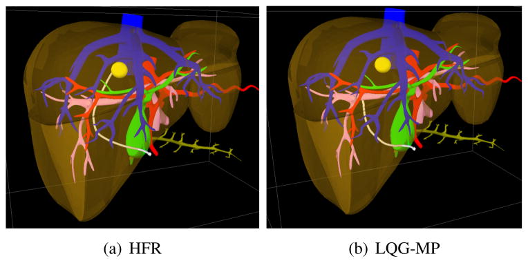
HFR applied in simulation to medical needle steering in the liver for a biopsy procedure at a different site from Fig. 1. The needle is inserted from the front. (a) HFR successfully guides the needle (white) to the tumor (yellow). Using LQG-MP (b), the needle collides with portal veins (pink).

Fig. 11.

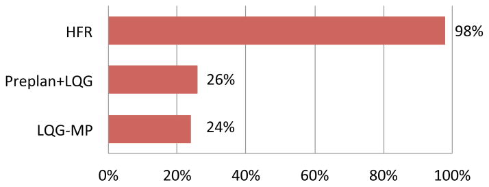
The percent of successful executions (i.e., reaching the goal and no collisions with obstacles) for the HFR, Preplan+LQG, and LQG-MP for the steerable needle liver biopsy scenario.

VII. Conclusion

As sampling-based motion planners become faster, they can be re-executed more frequently by a robot during task execution to react to uncertainty in robot motion, obstacle motion, sensing noise, and uncertainty in the robot’s kinematic model. We investigated and analyzed high-frequency replanning (HFR) for discrete-time systems with stochastic nonlinear (but linearizable) dynamics and observation models with noise drawn from zero mean Gaussian distributions. In HFR, during each period, RRT-based motion planners are executed in parallel as the robot simultaneously executes the first action of the best motion plan from the previous period. We considered two objectives relevant to problems with uncertainty: maximizing the probability of success (i.e., avoid collision with obstacles and reach the goal) and minimizing path length subject to a lower bound on the probability of success. We show that, as parallel computation power increases, HFR offers asymptotic optimality for these objectives during each period for goal-oriented problems. We demonstrated the effectiveness of HFR for three scenarios: (1) maneuvering a holonomic robot to a goal while avoiding moving obstacles, (2) steering a nonholonomic car-like robot with motion and sensing uncertainty, and (3) autonomously guiding a nonholonomic steerable medical needle whose curvature in different tissues types is not known a priori.

In ongoing and future work we would like to integrate new uncertainty-based cost functions with the HFR framework. One limitation of our current cost functions for considering uncertainty is that they assume Gaussian distributions. Although Gaussian distributions are commonly used for modeling uncertainty in a broad class of problems, they are not an acceptable approximation in some domains, such as problems in which uncertainty has a multi-modal distribution. For non-Gaussian problems, we will consider integrating particle filter approaches with the HFR framework. We also plan to investigate cost functions that efficiently estimate the probability of collision for geometrically complex robots, which will enable HFR to be used effectively for articulated manipulators. With the above future work, we hope to extend the applicability of the HFR approach to a broader class of robots.

Biographies

Wen Sun received his B.Tech degree in Computer Science and Technology from Zhejiang University, China, in 2012, a B.S. degree with Distinction in the School of Computing Science from Simon Fraser University, Canada, in 2012, and a M.S. degree in Computer Science from University of North Carolina at Chapel Hill, USA. He is currently a graduate student in Robotics Institute, Carnegie Mellon University. His research interests include motion planning under uncertainty and medical robotics.

Sachin Patil received his B.Tech degree in Computer Science and Engineering from the Indian Institute of Technology, Bombay in 2006 and the Ph.D. degree in Computer Science from the University of North Carolina at Chapel Hill in 2013. He is currently a postdoctoral researcher at UC Berkeley. His research interests include motion and path planning in virtual environments, physically-based simulation, and medical robotics.

Ron Alterovitz received his B.S. degree with Honors from Caltech, Pasadena, CA in 2001 and the Ph.D. degree in Industrial Engineering and Operations Research at the University of California, Berkeley, CA in 2006.

In 2009, he joined the faculty of the Department of Computer Science at the University of North Carolina at Chapel Hill, NC, where he leads the Computational Robotics Research Group. His research focuses on motion planning for medical and assistive robots. Prof. Alterovitz has co-authored a book on Motion Planning in Medicine, was awarded a patent for a medical device, has received multiple best paper finalist awards at IEEE robotics conferences, and is the recipient of the NIH Ruth L. Kirschstein National Research Service Award and the NSF CAREER Award.

References

- 1.Aghamohammadi A-a, Chakravorty S, Amato NM. Sampling-based nonholonomic motion planning in belief space via dynamic feedback linearization-based FIRM. Proc. IEEE/RSJ Int. Conf. Intelligent Robots and Systems (IROS); Oct. 2012; pp. 4433–4440. [Google Scholar]
- 2.Alterovitz R, Siméon T, Goldberg K. Robotics: Science and Systems (RSS) Jun, 2007. The Stochastic Motion Roadmap: A sampling framework for planning with Markov motion uncertainty. [Google Scholar]
- 3.Bialkowski JJ, Karaman S, Frazzoli E. Massively parallelizing the RRT and the RRT*. Proc. IEEE/RSJ Int. Conf. Intelligent Robots and Systems (IROS); San Francisco, CA. Sep. 2011; pp. 3513–3518. [Google Scholar]
- 4.Bry A, Roy N. Rapidly-exploring random belief trees for motion planning under uncertainty. Proc. IEEE Int. Conf. Robotics and Automation (ICRA); May 2011; pp. 723–730. [Google Scholar]
- 5.Carpin S, Pagello E. On parallel RRTs for multi-robot systems. Proc. 8th Conf. Italian Association for Artificial Intelligence; 2002. [Google Scholar]
- 6.Choset H, Lynch KM, Hutchinson SA, Kantor GA, Burgard W, Kavraki LE, Thrun S. Principles of Robot Motion: Theory, Algorithms, and Implementations. MIT Press; 2005. [Google Scholar]
- 7.Devaurs D, Siméon T, Cortés J. Parallelizing RRT on large-scale distributed-memory architectures. IEEE Trans Robotics. 2013 Apr;29(2):767–770. [Google Scholar]
- 8.Du Toit NE. PhD dissertation. California Institute of Technology; 2010. Robot Motion Planning in Dynamic, Cluttered, and Uncertain Environments: the Partially Closed-Loop Receding Horizon Control Approach. [Google Scholar]
- 9.Du Toit NE, Burdick JW. Robot motion planning in dynamic, uncertain environments. IEEE Trans Robotics. 2012 Feb;28(1):101–115. [Google Scholar]
- 10.Esposito JM, Kim J, Kumar V. Algorithmic Foundations of Robotics VI, ser. Springer Tracts in Advanced Robotics (STAR) Vol. 17. Springer; 2005. Adaptive RRTs for validating hybrid robotic control systems; pp. 107–122. [Google Scholar]
- 11.Gammell JD, Srinivasa SS, Barfoot TD. Informed RRT*: Optimal sampling-based path planning focused via direct sampling of an admissible ellipsoidal heuristic. In: Erdmann M, et al., editors. Proc IEEE/RSJ Int Conf Intelligent Robots and Systems (IROS) Sep, 2014. pp. 2997–3004. [Google Scholar]
- 12.Grimmett G, Stirzaker D. Probability and Random Processes. 3. New York: Oxford University Press; 2001. [Google Scholar]
- 13.Hauser K. Randomized belief-space replanning in partially-observable continuous spaces. In: Hsu D, et al., editors. Algorithmic Foundations of Robotics IX (Proc WAFR 2010), ser Springer Tracts in Advanced Robotics. Vol. 68. Springer-Verlag; Dec, 2010. pp. 193–209. [Google Scholar]
- 14.Hauser K. On responsiveness, safety, and completeness in real-time motion planning. Autonomous Robots. 2011 Sep;32(1):35–48. [Google Scholar]
- 15.Ichnowski J, Alterovitz R. Scalable multicore motion planning using lock-free concurrency. IEEE Trans Robotics. 2014 Oct;30(5):1123–1136. doi: 10.1109/TRO.2014.2331091. [DOI] [PMC free article] [PubMed] [Google Scholar]
- 16.Janson L, Pavone M. Fast marching trees: a fast marching sampling-based method for optimal motion planning in many dimensions. Int. Symp. Robotics Research (ISRR); Dec. 2013; [DOI] [PMC free article] [PubMed] [Google Scholar]
- 17.Karaman S, Frazzoli E. Sampling-based algorithms for optimal motion planning. Int J Robotics Research. 2011 Jun;30(7):846–894. [Google Scholar]
- 18.Kavraki LE, Kolountzakis MN, Latombe JC. Analysis of probabilistic roadmaps for path planning. IEEE Trans Robotics and Automation. 1998 Feb;14(1):166–171. [Google Scholar]
- 19.Koenig S, Likhachev M. Fast replanning for navigation in unknown terrain. IEEE Trans Robotics. 2005 Jun;21(3):354–363. [Google Scholar]
- 20.Kurniawati H, Hsu D, Lee W. Robotics: Science and Systems (RSS) Jun, 2008. SARSOP: Efficient point-based POMDP planning by approximating optimally reachable belief spaces. [Google Scholar]
- 21.LaValle SM, Kuffner JJ. Rapidly-exploring random trees: Progress and prospects. In: Donald BR, et al., editors. Algorithmic and Computational Robotics: New Directions. Natick, MA: AK Peters; 2001. pp. 293–308. [Google Scholar]
- 22.LaValle SM. Planning Algorithms. Cambridge, U.K: Cambridge University Press; 2006. [Google Scholar]
- 23.Littlefield Z, Li Y, Bekris KE. Efficient Sampling-based Motion Planning with Asymptotic Near-Optimality Guarantees for Systems with Dynamics. Proc. IEEE/RSJ Int. Conf. Intelligent Robots and Systems (IROS); Nov. 2013; pp. 1779–1785. [Google Scholar]
- 24.Luders BD, Karaman S, How JP. Robust sampling-based motion planning with asymptotic optimality guarantees. AIAA Guidance, Navigation, and Control (GNC) Conference; Aug. 2013; pp. 1–25. [Google Scholar]
- 25.Majumdar A, Tedrake R. Robust online motion planning with regions of finite time invariance. Proc. Workshop on the Algorithmic Foundations of Robotics (WAFR); 2012. [Google Scholar]
- 26.Melchior N, Simmons R. Particle RRT for path planning with uncertainty. Proc. IEEE Int. Conf. Robotics and Automation (ICRA); Apr. 2007; pp. 1617–1624. [Google Scholar]
- 27.Minhas D, Engh JA, Fenske MM, Riviere C. Modeling of needle steering via duty-cycled spinning. Proc. Int. Conf. IEEE Engineering in Medicine and Biology Society (EMBS); Aug. 2007; pp. 2756–2759. [DOI] [PubMed] [Google Scholar]
- 28.Otte M, Correll N. C-FOREST: Parallel shortest path planning with superlinear speedup. IEEE Trans Robotics. 2013 Jun;29(3):798–806. [Google Scholar]
- 29.Park C, Pan J, Manocha D. Real-time optimization-based planning in dynamic environments using GPUs. Proc. IEEE Int. Conf. Robotics and Automation (ICRA); May 2013; pp. 4090–4097. [Google Scholar]
- 30.Patil S, Alterovitz R. Interactive motion planning for steerable needles in 3D environments with obstacles. Proc. IEEE RAS/EMBS Int. Conf. Biomedical Robotics and Biomechatronics (BioRob); Sep. 2010; pp. 893–899. [DOI] [PMC free article] [PubMed] [Google Scholar]
- 31.Patil S, Burgner J, Webster RJ, III, Alterovitz R. Needle steering in 3-D via rapid replanning. IEEE Trans Robotics. 2014 Aug;30(4):853–864. doi: 10.1109/TRO.2014.2307633. [DOI] [PMC free article] [PubMed] [Google Scholar]
- 32.Patil S, Kahn G, Laskey M, Schulman J, Goldberg K, Abbeel P. Scaling up Gaussian belief space planning through covariance-free trajectory optimization and automatic differentiation. Proc. Workshop on the Algorithmic Foundations of Robotics (WAFR); Aug. 2014. [Google Scholar]
- 33.Patil S, van den Berg J, Alterovitz R. Estimating probability of collision for safe motion planning under Gaussian motion and sensing uncertainty. Proc. IEEE Int. Conf. Robotics and Automation (ICRA); May 2012; pp. 3238–3244. [Google Scholar]
- 34.Petti S, Fraichard T. Safe motion planning in dynamic environments. Proc. IEEE/RSJ Int. Conf. Intelligent Robots and Systems (IROS); Aug. 2005; pp. 2210–2215. [Google Scholar]
- 35.Plaku E, Kavraki L. Distributed sampling-based roadmap of trees for large-scale motion planning. Proc. IEEE Int. Conf. Robotics and Automation (ICRA); Apr. 2005; pp. 3868–3873. [Google Scholar]
- 36.Platt R, Jr, Tedrake R, Kaelbling L, Lozano-Perez T. Robotics: Science and Systems (RSS) Jun, 2010. Belief space planning assuming maximum likelihood observations. [Google Scholar]
- 37.Prentice S, Roy N. The belief roadmap: Efficient planning in belief space by factoring the covariance. Int J Robotics Research. 2009 Nov;28(11):1448–1465. [Google Scholar]
- 38.Rawlings J. Tutorial overview of model predictive control. IEEE Control Systems. 2000 Jun;20(3):38–52. [Google Scholar]
- 39.Reed KB, Majewicz A, Kallem V, Alterovitz R, Goldberg K, Cowan NJ, Okamura AM. Robot-assisted needle steering. IEEE Robotics and Automation Magazine. 2011 Dec;18(4):35–46. doi: 10.1109/MRA.2011.942997. [DOI] [PMC free article] [PubMed] [Google Scholar]
- 40.Stengel RF. Optimal Control and Estimation. Toronto, Canada: General Publishing Company, Ltd; 1994. [Google Scholar]
- 41.Sun W, van den Berg J, Alterovitz R. Stochastic Extended LQR: Optimization-based motion planning under uncertainty. Proc. Workshop on the Algorithmic Foundations of Robotics (WAFR); Aug. 2014; [DOI] [PMC free article] [PubMed] [Google Scholar]
- 42.van den Berg J, Abbeel P, Goldberg K. LQG-MP: Optimized path planning for robots with motion uncertainty and imperfect state information. Int J Robotics Research. 2011 Jun;30(7):895–913. [Google Scholar]
- 43.van den Berg J, Patil S, Alterovitz R. Motion planning under uncertainty using iterative local optimization in belief space. Int J Robotics Research. 2012 Sep;31(11):1263–1278. [Google Scholar]
- 44.van den Berg J, Patil S, Alterovitz R, Abbeel P, Goldberg K. LQG-based planning, sensing, and control of steerable needles. In: Hsu D, et al., editors. Algorithmic Foundations of Robotics IX (Proc WAFR 2010), ser Springer Tracts in Advanced Robotics (STAR) Vol. 68. Springer; Dec, 2010. pp. 373–389. [Google Scholar]
- 45.Vannoy J, Xiao J. Real-time adaptive motion planning (RAMP) of mobile manipulators in dynamic environments with unforeseen changes. IEEE Trans Robotics. 2008 Oct;24(5):1199–1212. [Google Scholar]
- 46.Vitus MP, Tomlin CJ. Closed-loop belief space planning for linear, Gaussian systems. Proc. IEEE Int. Conf. Robotics and Automation (ICRA); May 2011; pp. 2152–2159. [Google Scholar]
- 47.Wedge N, Branicky M. On heavy-tailed runtimes and restarts in rapidly-exploring random trees. AAAI Conference Workshop on Search in Artificial Intelligence and Robotics; Jul. 2008; pp. 127–133. [Google Scholar]
- 48.Yoshida E, Kanehiro F. Reactive robot motion using path replanning and deformation. IEEE Int. Conf. Robotics and Automation (ICRA); May 2011; pp. 5456–5462. [Google Scholar]
- 49.Zucker M, Kuffner J, Branicky M. Multipartite RRTs for rapid replanning in dynamic environments. Proc. IEEE Int. Conf. Robotics and Automation (ICRA); Apr. 2007; pp. 1603–1609. [Google Scholar]