Myocardial Perfusion Analysis in Cardiac Computed Tomography Angiographic Images at Rest

Abstract

Cardiac computed tomography angiography (CTA) is a non-invasive method for anatomic evaluation of coronary artery stenoses. However, CTA is prone to artifacts that reduce the diagnostic accuracy to identify stenoses. Further, CTA does not allow for determination of the physiologic significance of the visualized stenoses. In this paper, we propose a new system to determine the physiologic manifestation of coronary stenoses by assessment of myocardial perfusion from typically acquired CTA images at rest. As a first step, we develop an automated segmentation method to delineate the left ventricle. Both endocardium and epicardium are compactly modeled with subdivision surfaces and coupled by explicit thickness representation. After initialization with five anatomical landmarks, the model is adapted to a target image by deformation increments including control vertex displacements and thickness variations guided by trained AdaBoost classifiers, and regularized by a prior of deformation increments from principal component analysis (PCA). The evaluation using a 5-fold cross-validation demonstrates the overall segmentation error to be 1.00±0.39mm for endocardium and 1.06±0.43mm for epicardium, with a boundary contour alignment error of 2.79±0.52. Based on our LV model, two types of myocardial perfusion analyses have been performed. One is a perfusion network analysis, which explores the correlation (as network edges) pattern of perfusion between all pairs of myocardial segments (as network nodes) defined in AHA 17-segment model. We find perfusion network display different patterns in the normal and disease groups, as divided by whether significant coronary stenosis is present in quantitative coronary angiography (QCA). The other analysis is a clinical validation assessment of the ability of the developed algorithm to predict whether a patient has significant coronary stenosis when referenced to an invasive QCA ground truth standard. By training three machine learning techniques using three features of normalized perfusion intensity, transmural perfusion ratio, and myocardial wall thickness, we demonstrate AdaBoost to be slightly better than Naive Bayes and Random Forest by the area under receiver operating characteristics (ROC) curve. For the AdaBoost algorithm, an optimal cut-point reveals an accuracy of 0.70, with sensitivity and specificity of 0.79 and 0.64, respectively. Our study shows perfusion analysis from CTA images acquired at rest is useful for providing physiologic information in diagnosis of obstructive coronary artery stenoses.

Graphical Abstract

1. Introduction

Despite improvements in therapies targeted at reducing disease burden, coronary artery disease (CAD) continues to afflict >16 million US adults, accounting for more than 1/3 of all deaths and responsible for ~1.2 million hospitalizations annually (Lloyd-Jones et al., 2010). Numerous non-invasive physiologic imaging tests exist for assessment of CAD, including echocardiography, magnetic resonance imaging (MRI) and myocardial perfusion scintigraphy by either single photon emission computed tomography (SPECT) or positron emission tomography (PET) (Berman et al., 2006)(Gershlick et al., 2007). These modalities identify stress-induced wall motion abnormalities or regional myocardial perfusion defects to determine individuals who may have severe coronary stenoses. Recently, computed tomography (CT) of >64-detector rows has become a promising non-invasive option for coronary angiography, now allowing for acquiring virtually motion-free images at isotropic spatial resolution of 0.5mm in a few seconds (Min et al., 2010).

Compared to an invasive reference standard, coronary CT angiography (CTA) demonstrates excellent diagnostic performance in stenosis detection (Budoff et al., 2008). Yet CTA is prone to artifacts—including those from motion, beam hardening and mis-registration—which reduce the diagnostic accuracy of CTA. Further, CTA is prone to overestimation of stenosis severity and more recent data has suggested that an anatomic stenosis visualized on CTA is not necessarily associated with interruption of coronary blood flow. Quantitative coronary angiography (QCA) is the most common clinical reference standard to determine the diameter percentage of luminal stenosis, which is performed by computer-assisted calculation of the ratio of the minimal lumen diameter of a stenosis to the reference vessel diameter on conventional X-ray angiographic images (Reiber et al., 1984). Fractional flow reserve (FFR) is an emerging reference standard to determine if a stenosis significantly limits the blood flow, which is defined by the ratio of maximal blood flow distal to a stenosis to normal maximal flow in the same vessel (Pijls et al., 1996). However, both tests require invasive insertion of a catheter in the artery and thus should only be used when necessary. To identify functionally significant stenoses non-invasively, new computational and imaging methods have been developed. For example, a technique to compute FFR by computational fluid dynamics has been shown to improve diagnostic performance over using CTA alone (Taylor et al., 2013), yet it requires lengthy processing times and is unable to reveal abnormal myocardial perfusion caused by microvascular diseases. Stress CT perfusion imaging shows great promise in this area but requires additional imaging sessions thus leads to increased radiation exposure (George et al., 2006).

No previous work has been performed to determine the diagnostic value of myocardial perfusion quantified using CTA alone acquired at rest. This is desirable if myocardial perfusion noninvasively evaluated at rest provides useful information about the severity of coronary artery lesions while requiring no additional imaging. In this regard, automated and quantitative analysis of myocardial perfusion is ideal to maximize diagnostic accuracy, reduce burden of manual interpretations and enhance objectivity and reproducibility of such analyses. Previous CT perfusion analyses have been primarily carried out manually (Mehra et al., 2011), while sometimes assisted by semi-automated tools (George et al., 2006)(George et al., 2009)(Kachenoura et al., 2009). Automatic and fast methods to quantify perfusion abnormalities have been lacking. Precise delineation of endocardium and epicardium of the left ventricle (LV) is mandatory for accurate perfusion analysis because false detection may occur in intraventricular or pericardial regions with low or high attenuation densities. In contrast, all previous studies followed straightforward approaches to define presence and severity of a perfusion deficit, either by visual inspection with the help of a chosen window level or quantification using a defined threshold. However, the distribution of CT perfusion intensity varies significantly in different regions of the myocardium within a group of normal subjects (shown in Fig. 1). Because of low contrast, it is generally difficult to reliably distinguish a hypoattenuated area from neighboring normal regions. In addition, several confounding factors—including noise or other artifacts—can resemble or hide perfusion abnormalities. Beam hardening is one of the most common ones, and causes hypoattenuated shadowing effects within the myocardium. Therefore, the use of a global window level or threshold is indeed questionable. Furthermore, no consensus has been presently established as the optimal variable to characterize perfusion defects, which leads to multiple possibilities.

Fig. 1.

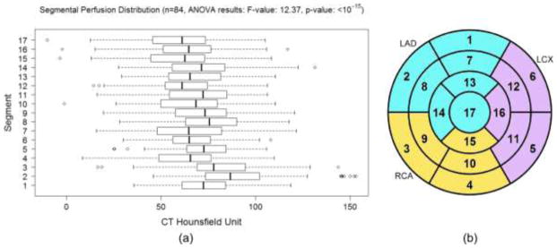
(a) The difference of segmental myocardial perfusion distribution in normal patients (without 50% coronary stenosis defined by QCA). With correction for multiple comparison, the pairs with significant differences (p-value<0.005) are 2-17, 2-15, 2-12, 2-4, 2-16, 2-7, 2-13, 2-10, 2-6, 3-17, 3-15, 2-11, 2-14, 2-9, 3-12, 2-5, 8-17, 8-15, 2-1, 3-4, 3-16, 8-12, 3-7, 1-17, 1-15, 2-8, 5-17, 3-13, 5-15, 3-10, 3-6, 8-4, 8-16, 9-17, 9-15, 14-17, 14-15, 1-12, 5-12. (b) AHA 17-segment model with territory assigned to left anterior descending (LAD), left circumflex (LCX), and right coronary (RCA) arteries.

In this study, we propose a new system to analyze myocardial perfusion using CTA alone acquired at a rest state and assess its diagnostic value to identify severe coronary lesions that cause myocardial perfusion deficits. Our myocardial perfusion analysis is based on the contrast enhancement information in CTA images, instead of absolute myocardial perfusion (in ml/min/g), which is not available in a single resting scan. From CTA images, we develop a compact representation of LV by subdivision surfaces, which ensure the smoothness even with small number of vertices. The thickness of the myocardium is explicitly modeled in this representation, enabling the coupling between endocardial and epicardial layers. We then divide the myocardium automatically into American Heart Association (AHA) 17-segment model (Cerqueira, 2002) using mesh parameterization. We perform two independent studies to assess the usefulness of quantifying myocardial perfusion from different perspectives. Using a new concept of perfusion network analysis, we measure the degree of correlations of perfusion among different segments in order to assess the heterogeneous perfusion network structure exhibiting in normal subjects, as well as the disturbed perfusion network in the diseased subjects. Finally, normalized perfusion intensity, transmural perfusion ratio, and myocardial wall thickness are calculated in all segments as features, and the ability to predict the existence or absence of a significant coronary stenosis is explored using machine learning techniques. Our key contributions are threefold:

1. LV segmentation: Based on the subdivision surfaces and machine learning, our new method allows both automatic segmentation and interactive editing of LV surfaces. Our model has significantly fewer control points than previous methods, which allows for faster automatic fitting. We support interactive editing by allowing the user to drag the control points of LV surfaces and modify the thickness associated with any control point. In this paper, interactive editing was used to generate manual annotations, but all the evaluation results are only based on automatic segmentation. The explicit thickness representation allows precise thickness measurements by ensuring the segment between corresponding points on endocardial and epicardial surfaces is always perpendicular to the mid-epicardial surface. The mapping from a 3D myocardial model into an AHA model is driven by mesh parameterization as opposed to most conventional techniques of planar cutting, and thus ensuring better coverage in the basal regions. Finally, our principal component analysis (PCA) prior of deformation increments, avoids the need to run Procrustes analysis and is concise, reducing the degrees of freedom (3D coordinates on both surfaces) per point from 6 to 2 (normal displacement and thickness for internal vertices and normal and tangent displacements for boundary vertices).

2. Network analysis: The coronary vascular tree provides essential blood flow to the myocardium. Under normal physiologic conditions, coronary flow is well maintained to satisfy the metabolic demand of myocardial tissue. The rate of perfusion through the myocardium is driven by aortic pressure and controlled by the morphology and resistance of distal vascular beds. Inspired by widely recognized functional connectivity among different regions of brain during rest and task-related activities (Greicius et al., 2003)(Buckner et al., 2008), we propose a new concept to create a rest perfusion network by characterizing the correlation relationship of myocardial perfusion among different myocardial regions. We compare the structure of the perfusion network in the normal and diseased group of patients and identify differences in network patterns.

3. Prediction analysis: It is well known from SPECT and MRI studies that perfusion defects visualized in the rest scans are associated with severe ischemia or infarction. However, the ability of using rest CT perfusion to predict ischemia-causing coronary lesions that are identified by invasive QCA has not been explored. For the first time, we evaluate myocardial perfusion and thickness quantitation from noninvasive CTA to predict patients with high-grade disease by invasive QCA using machine learning techniques. We show the invasive measurements are indeed predictable and the performance of prediction is carefully evaluated.

2. Related Work

2.1 Automated 3D Segmentation of the Heart from CT Images

Numerous algorithms for 3D heart segmentation have been published in the past. We refer the readers to a survey in (Frangi et al., 2001) for the early work in this area, especially for SPECT, MR, and Ultrasound. We will focus on a summary of existing methods for automated segmentation of the heart from CT images (Kang et al., 2012). Two major approaches have been proposed. One is model-based, in which a template mesh model is first transformed to the proximity of the target heart in the new image and then the model is adjusted to fit the boundary. From the landmark work in (Lorenz and von Berg, 2006), a comprehensive heart model including four chambers and trunks of the attached vessels were constructed semi-automatically by landmark-driven model initialization and energy-minimizing surface adaption. In (Ecabert et al., 2008), whole heart segmentation was introduced, in which generalized Hough transform was used to localize the heart. Parametric and deformable adaptations were then performed to match the heart boundary. This work has been extended to segment the attached great vessels (Ecabert et al., 2011). In (Zheng et al., 2008), four-chamber heart segmentation was proposed. Learning-based methods were described to search the similarity transform to locate the heart and delineate the boundary. The other approach of heart segmentation is atlas-based, in which manual labels of segmented atlas images are propagated into the new image by image registration and the final segmentation is obtained by a voting procedure at each voxel. In (Isgum et al., 2009), whole heart regions were isolated from chest CT scans using multiple atlases and the local votes were derived from local assessment of the registration success. In (van Rikxoort et al., 2010), the same task was performed by selecting the most appropriate atlases and locally deciding a subset of atlases are needed. In (Kirişli et al., 2010), a multi-atlas heart and chamber segmentation method was evaluated on a large number of patients. In (Hoogendoorn et al., 2013), a detailed atlas and spatio-temporal statistical model of the human heart based on a large population of 3D+time CT sequences by registering a synthesized population mean image to all subjects in the population. Although these methods have been proposed for automatic contouring for cardiac CT imaging data to statistically analyze cardiac shapes as well as measure cardiac function such as stroke volume, injection fraction, and thickness, their utility and accuracy of defining myocardial regions for perfusion analysis have not been evaluated.

2.2 Myocardial Perfusion Analysis from CT Images

Cardiac CT perfusion imaging is a novel non-invasive technique to assess the blood flow to the myocardium, originating from the seminal work in (George et al., 2006)(George et al., 2009). When adding this essential physiologic information to traditional anatomical assessment of CAD, CT perfusion leads to a new rationale for comprehensive evaluation using only one modality. A typical CT perfusion protocol includes image acquisition under stress and rest states. By visual inspection, a myocardial region with perfusion defects shows low contrast concentration. By comparing the same region under the two states, reversible or fixed perfusion defects can be distinguished (Techasith and Cury, 2011). CT perfusion analysis is primarily performed by visual inspection of hypoattenuated areas in the myocardium using user-defined window levels and slice thickness. In most studies, the existence and severity of perfusion defects is qualitatively graded into categorical variables (Blankstein et al., 2009)(Ko et al., 2012). In some studies, normal myocardial attenuation of the patient as an internal reference (Tamarappoo et al., 2010). Yet selection of this normal reference may be biased because the distribution of normal attenuation in each segment is different. Quantitative perfusion analysis is very limited. Transmural perfusion ratio was introduced in (George et al., 2009), which is defined as the ratio of mean attenuations in subendocardial to subepicardial layers. Another extent and severity of perfusion abnormality index was proposed by analyzing the histogram of attenuations within each segment and compared to a normal segment. In this paper, our focus is the analysis of myocardial perfusion at rest states, for which the scan protocol is equivalent to a typical CTA scan.

3. Materials and Methods

3.1 Data

From a previously completed clinical trial, we obtained 140 CTA images from 140 patients (Gender: 52.1% male, Age: 54.2±11.0). When multiple phases exist, the phase with best quality close to end-diastole was used. The data were acquired using standard coronary CTA protocol on either Siemens Definition or GE Discovery scanners. Image volumes may contain 153–357 slices, while the dimension of each slice is identically 512×512 pixels. For different volumes, the in-slice resolution is isotropic and varies between 0.28 to 0.49 mm with a slice thickness from 0.30 to 0.63 mm. Five landmarks and LV endocardial and epicardial surfaces in all volumes were manually annotated by several expert users, which was used as the ground-truth data for evaluating our automated LV segmentation algorithm. The manual annotations were generated using an in-house computer program by completely manual definition of the landmarks and LV segmentations. Any volume is only annotated by one user. Each patient also underwent invasive coronary angiography and the coronary tree was analyzed using a 19-segment coronary model on all coronary segments 2.0 mm in diameter. The percentage luminal diameter stenosis was visually and quantitatively graded in each segment and the degree of vessel obstruction for the patient or for each of LAD, LCX, and RCA territories by QCA (CAAS, Pie Medical Imaging, Maastricht, Netherlands) is calculated by the most severe obstruction of the attributed segments. The numbers of patients with 0–25%, 26–49%, 50–70%, and 71–100% stenoses by QCA are 17, 65, 27, and 31, respectively. To provide unbiased evaluation of landmark detection and LV segmentation, a separation set of 15 images (scanned with the same protocol and manual annotation process, in-slice resolution: 0.31 to 0.52 mm, slice thickness: 0.40 to 0.60 mm, 6 images with ≥50% stenoses by QCA) were used to determine the optimal parameters (e.g. the number of decision trees and maximal depths of each tree, etc.) for machine learning and the parameters were fixed when performing evaluations by cross-validation. To build the template model (in Section 3.4) used for LV segmentation, another representative image (scanned with the same protocol, in-slice resolution: 0.31 mm, slice thickness: 0.60 mm, with <50% stenosis by QCA) was used.

3.2 Left Ventricle Modeling

Triangular meshes have been predominantly used in model-based heart segmentation. We observe at least three limitations need improvements for the application of perfusion analysis:

3.2.1 The meshes are dense (e.g. 545 points in (Zheng et al., 2008))

This leads to more computation in automatic segmentation due to the additive computational cost associated with each mesh point. It may also cause mesh distortion in manual editing when the movement of individual mesh point intersects with neighing triangles.

3.2.2 Myocardial thickness is not explicitly modeled

Because the endocardial and epicardial surfaces are separately modeled, perpendicular directions through the myocardium cannot be defined by the corresponding vertices on both surfaces, leading to difficulty in thickness measurements and the split between endocardial and epicardial layers.

3.2.3 The basal portion of the myocardium is missing

Models with flat basal openings were sometimes used but a complete LV model is necessary since perfusion defects may exist at the base of the heart.

We represent the left ventricle model as a subdivision surface based on a control mesh = {V^C, E^C, Q^C}, where $V^C=\{{\mathit{v}}_1^C,{\mathit{v}}_2^C,\cdots ,{\mathit{v}}_{N_C}^C\}$ is a set of N_C control vertices, E^C is the edge connectivity, and Q^C is a collection of scalar or vector properties associated with each vertex. Many subdivision surface schemes have been developed, which differs in terms of the type of the control mesh (triangular or rectangular), the nature of fitting (interpolation or approximation), and the smoothness (C¹ or C² continuity). In the current work, a Loop subdivision scheme (shown in Fig. 2(a)) based on a triangular is used (Loop, 1987) because it is C² continuous everywhere except at extraordinary vertices, where they are C¹-continuous. Although it is an approximation scheme, our experiments showed it is more tolerant to vertex distortion than interpolation scheme, e.g. the Butterfly scheme. In Fig. 2(b), the weights to compute the finer surface in one step are shown for both internal and boundary vertices, in which two types of vertices are differentiated. Odd vertices are those newly inserted during subdivision, whereas even vertices are those exist in the previous subdivision step. Because the standard Loop weights are used for internal vertices, the corresponding vertices in do not lie on the subdivision surface. Nevertheless, we modify the weights for the boundary vertices to make the boundary curve always interpolate the control vertices on the boundary. Using the weights, a sequence of refined surfaces can be computed, = , , , ···. The relationship of vertex coordinates or other properties (e.g. thickness) between two subsequent refinements can be established by linear mapping:

$${\mathit{q}}^{j+1}=\mathcal{W}{\mathit{q}}^j,$$ (1)

where q^j and q^j+1 are vectors including properties (e.g. vertex coordinates and thickness) in all vertices of and , respectively. Note the dimension of q^j+1 is larger than q^j due to the insertion of new vertices. is a sparse matrix containing the weights. Conversely, if q^j+1 is known, q^j may be estimated by solving a least squares problem:

$${\widehat{\mathit{q}}}^j={\left({\mathcal{W}}^T\mathcal{W}\right)}^{-1}{\mathcal{W}}^T{\mathit{q}}^{j+1}$$ (2)

Fig. 2.

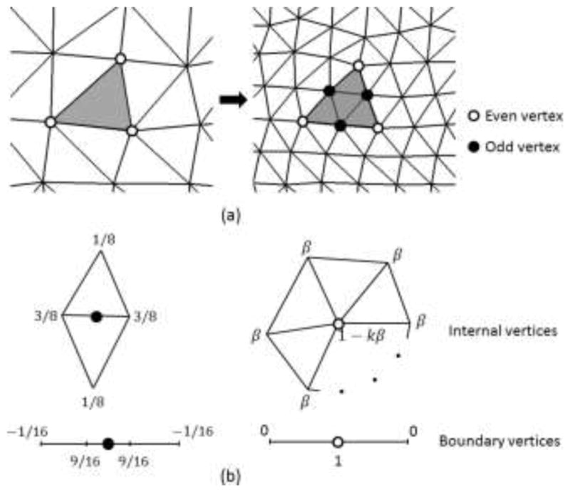
(a) The modified Loop subdivision scheme splits each triangle into four triangles. In each subdivision step, a new vertex is generated on each edge, denoted as odd vertex, whereas existing ones are even vertices. (b) The weights used to position internal and boundary vertices, where $\beta =\frac{1}{k}\left(\frac{5}{8}-{\left(\frac{3}{8}+\frac{1}{4}cos\frac{2\pi }{k}\right)}^2\right)$, and k is the number of incident vertices.

Strictly, the subdivision surface is the limit surface after an infinite number of refinements. In our experiments, was used for a good tradeoff between speed and accuracy. The LV model is shown in Fig. 3(a). In total, the control mesh has 86 vertices and 160 triangles. The thickness of the myocardium is explicitly modeled as one of the properties ${\mathit{\Theta }}^C=\{{\theta }_1^C,{\theta }_2^C,\cdots ,{\theta }_{N_C}^C\}\in Q^C$ associated with each vertex in . Three surfaces are delineated to split the myocardium into two layers, enclosed by mid-myocardial , endocardial , and epicardial surfaces, respectively. In our model, is set to . and are implicitly generated by warping inwards and outwards along normal directions by half of the thickness in (computed using Eq. (2)), respectively. The three surfaces coincide at a boundary contour by locally enforcing the thickness to be zero. The boundary contour consists of two curves. One follows mitral valve annulus and the other passes the aortic level. Using this representation, our LV model is uniquely defined by specifying two sets of parameters: coordinates $V^C=\{{\mathit{x}}_1^C,{\mathit{x}}_2^C,\cdots ,{\mathit{x}}_{N_C}^C\}$ and thickness ${\mathit{\Theta }}^C=\{{\theta }_1^C,{\theta }_2^C,\cdots ,{\theta }_{N_C}^C\}$ of the control vertices, which allows a user or an algorithm to fit the model to an image by interactively or automatically modifying these parameters.

Fig. 3.

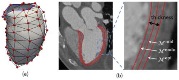
(a) LV model with the control mesh (vertices in red and edges in black). The blue boundary contour passes mitral valve annulus on one side and the aortic valve level on the other side. (b) The midcardial surface is modeled as subdivision surface. The endocardial and epicardial surfaces are represented by warping inwards and outwards along normal directions by half of the thickness each.

3.3 Overview of Automatic Left Ventricle Segmentation

The goal of automatic LV segmentation is then to determine {V^C, Θ^C} in a given image. Our segmentation algorithm has two steps (shown in Fig. 4): (1) LV initialization: Five anatomic landmarks are defined and automatically detected using trained classifiers. A template model is transformed by aligning the corresponding anatomic landmarks defined on the template and detected in the figures. (2) LV boundary delineation: The boundary of the transformed model is further refined to fit the actual LV boundary in the image by deformation increments including control vertex displacements and thickness variations guided by trained classifiers, and regularized by a prior of deformation increments from principal component analysis (PCA) analysis.

Fig. 4.

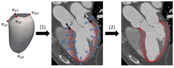
Overview of the automatic LV segmentation algorithm. (1) LV initialization by transforming a template model using landmark correspondences. (2) LV boundary delineation by adjusting internal vertices along n⃗ for and boundary vertices along both n⃗ and b⃗.

3.4 LV initialization by landmark detection and alignment

We reconstruct a template model from one representative image (described in Section 3.1). Five anatomic landmarks are defined on the model (which are also mesh vertices): v_AP is the apex point, v_MV is the midpoint along the mitral valve annulus curve, v_AV is the midpoint along the aortic valve level curve, v_AT and v_PT are the most anterior and posterior points on the boundary contour separating the two curves, respectively. We detect these landmarks in the image by learning-based using Haar-like wavelet features and an AdaBoost classifier for each landmark (100 decision trees with 5 maximal depth). Similar to (Zheng et al., 2008), the classifiers were used to scan through the whole image and the locations with maximal likelihoods was selected to the detected landmarks. The corresponding landmarks in the template space and in the image space allow us localize the LV in the image and transform the template model in the proximity of the true LV location to prepare for boundary delineation introduced in Section 3.5. An affine transform T is estimated in a least squares sense to best fit the detected landmarks in the image space when mapping from the template space. Let { $V_T^C,{\mathit{\Theta }}_T^C$} be the coordinates and thickness associated with the control vertices in the transformed model by T.

3.5 LV boundary delineation

The main goal of boundary delineation is to search for the best combination { $V_T^C,{\mathit{\Theta }}_T^C$} to make and fit the actual LV endocardial and epicardial boundaries. Because and directly relates to , it is more convenient to determine { $V_T^{\text{mid}},{\mathit{\Theta }}_T^{\text{mid}}$} on instead and then obtain { $V_T^C,{\mathit{\Theta }}_T^C$} through Eq. (2). Therefore, there are four unknown parameters for each vertex on . To save computational cost, we choose to only search for the even vertices that originate from . Although the vertices may be freely moved, constraints on the search directions must be enforced to avoid vertex distortion while achieving a good fit as shown in Fig. 4. For any vertex on , the normal vector n⃗ is well defined and used as the search direction. However, only searching in n⃗ may not result in an adequate fit for boundary vertices. For those vertices, we can define two vectors: t⃗ is the tangent vector of the boundary contour, and b⃗ = n⃗ × t⃗ is the binormal vector of the boundary contour. We allow the boundary vertices move along both n⃗ and b⃗, yet only n⃗ for internal vertices. Considering the constraints of zero thickness on the boundary vertices mentioned before, we reduce the number of unknown parameters for each vertex into two, namely the distance along n⃗ for all vertices Δn, the thickness change for internal vertices Δθ, and the distance along b⃗ for boundary vertices Δb.

We refer to the two parameters (i.e. Δn and Δθ for internal vertices, Δn and Δb for boundary vertices) for each vertex as deformation increments. To determine the deformation increments, a classifier is trained to capture the characteristics of the boundary appearance and search for the best fit in a new image. Let I(x) and ∇I(x) be the image intensity and gradient at a point x. As shown in Fig. 5, a feature vector is created which includes I, $\sqrt{\mid I\mid }$, I², I³, ∇I, $\sqrt{\mid \nabla I\mid }$, |∇I|², |∇I|³, ∇I · n⃗ sampled at each of the five points {x − θ · n⃗, $\mathit{x}-\frac{\theta }{2}·\overrightarrow{\mathit{n}}$, x, $\mathit{x}+\frac{\theta }{2}·\overrightarrow{\mathit{n}}$, x + θ · n⃗}. A sample used in training is positive only when both x and θ match ground truths and otherwise are negative. Negative samples are generated by varying ground truth x by a maximal distance of 20 voxels in both directions along n⃗ at increment of 1 voxel and varying ground-truth θ between 2 voxels and 5 times θ at an increment of 2 voxels. For boundary vertices, negative samples are also generated by a maximal distance of 20 voxels in both directions along b⃗ at increment of 1 voxel but with a fixed θ of 5 voxels. Positive and negative samples with their features are used to train an AdaBoost classifier to determine the deformation increments for each vertex, which lead to maximal class probabilities belonging to the true boundary:

Fig. 5.

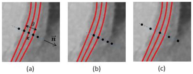
Feature extraction at five points (black dots) for a vertex x with thickness θ and surface normal n⃗. The red curves are endo-, mid-, and epicardial surfaces. (a) Positive sample with both ground-truths of x and θ. (b) (c) Negative samples with x or θ deviated from ground-truth.

• For internal vertices:

  $$\{{\widehat{\mathrm{\Delta }n}}_i,{\widehat{\mathrm{\Delta }\theta }}_i\}=arg\underset{\mathrm{\Delta }{n}_i,\mathrm{\Delta }{\theta }_i}{max}\sum _{{\mathit{v}}_j\in \mathcal{N}({\mathit{v}}_i)}{\mathcal{L}}_i({\mathit{v}}_j+\mathrm{\Delta }{n}_i·{\overline{\mathit{n}}}_j,{\theta }_j+\mathrm{\Delta }{\theta }_i)$$ (3)
• For boundary vertices:

  $$\{{\widehat{\mathrm{\Delta }n}}_i,{\widehat{\mathrm{\Delta }b}}_i\}=arg\underset{\mathrm{\Delta }{n}_i,\mathrm{\Delta }{b}_i}{max}\sum _{{\mathit{v}}_j\in \mathcal{N}({\mathit{v}}_i)}{\mathcal{L}}_i({\mathit{v}}_j+\mathrm{\Delta }{n}_i·{\overline{\mathit{n}}}_j,{\mathit{v}}_j+\mathrm{\Delta }{b}_i·{\overrightarrow{\mathit{b}}}_j),$$
  where v_i is the i-th vertex, v_j is a vertex in the one-ring neighborhood (v_i) of v_i on , and (·) is the probability belonging to the true boundary estimated by the classifier. Note we train one classifier for each vertex to account for the considerable spatial appearance difference. Equation (3) generally performs well when the boundary is strong. However, it may lead to false negatives in case of weak boundaries. We alleviate this problem by enforcing a prior of deformation increments by PCA:

  $$\stackrel{\sim }{\mathit{\varphi }}=\overline{\mathit{\varphi }}+\sum _{k=1}^K{t}_k{\mathbf{\Phi }}_k,$$ (4)

  where $\stackrel{\sim }{\mathit{\varphi }}=\{\cdots \cdots ({\stackrel{\sim }{\mathrm{\Delta }n}}_i,{\stackrel{\sim }{\mathrm{\Delta }\theta }}_i\text{or}{\stackrel{\sim }{\mathrm{\Delta }b}}_i)\cdots \cdots \}$ is the vector of all deformation increments projected into PCA subspace, ϕ̄ is the mean of all samples of ϕ in the training data, Φ_k the eigenvector corresponding to the k-th largest eigenvalue, and t_k is the coefficient. We retain the largest K which captures 98% of total variance in our experiment. To generate the training data, we utilized ${\mathcal{M}}_{\text{truth}}^{\text{mid}}$ from manually annotated ground-truths and the deformation increments can be obtained (shown in Fig. 6) by calculating the difference between ${\mathcal{M}}_{\text{truth}}^{\text{mid}}$ and ${\mathcal{M}}_{\text{init}}^{\text{mid}}$, the latter of which is initialized with manually identified landmarks. Specifically, we search in both directions of n⃗ for any internal vertex x_init of ${\mathcal{M}}_{\text{init}}^{\text{mid}}$ for the intersection point x_truth on ${\mathcal{M}}_{\text{truth}}^{\text{mid}}$. Then, Δn is the signed distance between x_truth and x_init and Δθ is the thickness difference. For any boundary vertex of ${\mathcal{M}}_{\text{init}}^{\text{mid}}$, we search for the closest point on the boundary contour of ${\mathcal{M}}_{\text{truth}}^{\text{mid}}$and project this vector on n⃗ and b⃗ to get Δn and Δb. The corrected deformation increments ϕ̃ is then used to determine {V^C, Θ^C} of the control mesh using Eq. (2).

Fig. 6.

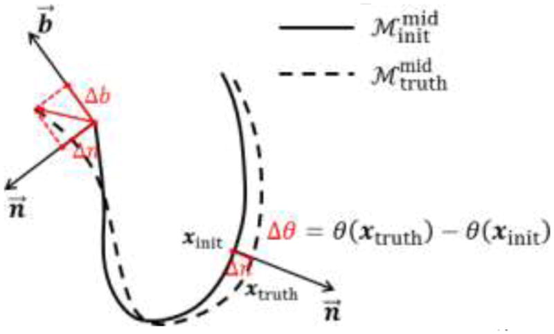
Generation of training data for PCA analysis of deformation increments. ${\mathcal{M}}_{\text{init}}^{\text{mid}}$ and ${\mathcal{M}}_{\text{truth}}^{\text{mid}}$ are after LV initialization using manually identified landmarks and from manually annotated ground-truth surface.

3.6 Perfusion Network Analysis

Using the AHA 17-segment model, we subdivide the myocardium and quantify perfusions in each segment. In order to subdivide our LV model, we parameterize by assigning {u, v} coordinates to every control vertices. The {u, v} coordinates of vertices on the boundary contour are fixed on a unit circle. The vertex corresponding to the apex point is assigned to {0,0}. The {u, v} coordinates of all other control vertices are assigned based on weighting the ratio between the geodesic distances from the vertex to the boundary contour d_BC and to the apex d_AP and rotating by the relative angle φ along the LV short axis, i.e. $\{\mathrm{u},\mathrm{v}\}=\{\frac{{\mathrm{d}}_{\text{AP}}}{{\mathrm{d}}_{\text{AP}}+{\mathrm{d}}_{\text{BC}}}cos\varphi ,\frac{{\mathrm{d}}_{\text{AP}}}{{\mathrm{d}}_{\text{AP}}+{\mathrm{d}}_{\text{BC}}}sin\varphi \}$. The parameterization of can be computed using Eq. (1). As shown in Fig. 7, the {u, v} coordinates can be used to subdivide into 17 segments S_i, i = 1,2, ···,17. To quantify perfusion in a segment P_Si, we first average the image intensities of any point x (with thickness θ and normal n⃗) on the line segment between $\mathit{x}-\frac{\theta }{2}\overrightarrow{\mathit{n}}$ and $\mathit{x}+\frac{\theta }{2}\overrightarrow{\mathit{n}}$, and then average over all points belonging to S_i.

Fig. 7.

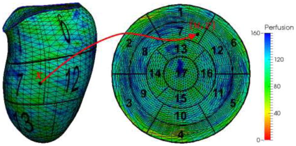
Mapping between a 3D point x on to a 2D point {u, v} within a unit circle. The perfusion for any point is calculated by averaging the image intensities within the thickness in both directions along normal.

To characterize contrast concentration in the proximal ascending aorta (right after aortic valve) and the LV blood pool (in the mid cavity), we also compute the medians of image intensities P_Aorta and P_LV within two spherical regions of locations and sizes automatically adjusted based on the LV geometry. Medians are used to reduce the influences of lower intensities caused by valves, chordae tendineae, or papillary muscles. We combine all intensity measurements in a vector P = {P_S1, P_S2, ··· P_S17, P_Aorta, P_LV}. Note these measurements are directly calculated from image intensities without any normalization. The correlation matrix (P) is defined by computing Pearson correlation coefficients among all pairs considering each patient as one sample. The perfusion network is constructed by analyzing the strength of correlation relationship (as network edge) between each perfusion measurement in P (as network node). Large positive correlation shows a strong agreement in the level of perfusion between a pair of myocardial regions, i.e. being hyperperfusion or hypoperfusion together frequently. Low correlation may indicate perfusion in two regions are independent or lack linear dependence, i.e. one being hyperperfusion, while the other being hypoperfusion frequently. The latter can happen naturally or be disturbed by disease, e.g. ischemia or myocardial infarction. It should be emphasized that our perfusion network analysis is based on information obtained during the short period when CTA data were acquired. The nature of our data does not allow us to analyze temporal relationship. The method of dynamic helical CT imaging may permit a temporal analysis but requires significantly increased radiation exposure to the patient and thus is not favored. We also note the strong correlation may or may not indicate the two regions are adjacent or the blood flow is supplied by the same coronary artery. To reveal the disease-induced changes in the perfusion network, the topology and connectivity strength can be compared between two groups of patients discriminated by QCA results:

1. Normal group: Patients with <50% luminal stenosis.

2. Disease group: Patients with ≥50% luminal stenosis.

3.7 Perfusion Prediction Analysis

Using machine learning techniques, we also assess the ability to predict the existence of significant coronary artery stenosis (≥50% luminal diameter reduction) suggested by invasive QCA by using myocardial perfusion and thickness from noninvasive CTA imaging at rest alone. Our work aims to elucidate how the information gained from noninvasive imaging informs the invasive measurements.

Specifically, we extract totally 51 features—three features in each of the 17 segments from the LV segmentation:

1. Normalized perfusion intensity (NPI): It is computed by first averaging the minimal image intensity on the line segment between $\mathit{x}-\frac{\theta }{2}\overrightarrow{\mathit{n}}$ and $\mathit{x}+\frac{\theta }{2}\overrightarrow{\mathit{n}}$ over all points belonging to S_i and then normalizing by dividing P_Aorta. Different from the perfusion computation in perfusion network analysis, we compute the minimal intensity on the line segment because it is known that stenosis-induced perfusion deficits often exhibit reduced image intensity. The normalization is performed to remove the dependence of the different absolute contrast concentration among patients. Essentially, both P_Aorta and P_LV can be used for this purpose because the high correlation between them. We use P_Aorta in our experiment.

2. Transmural perfusion ratio (TPI): It is the ratio of subendocardial perfusion to subepicardial perfusion. Subendocardial perfusion is computed by averaging the minimal image intensity on the line segment between x and $\mathit{x}-\frac{\theta }{2}\overrightarrow{\mathit{n}}$ over all points belonging to S_i. Epicardial perfusion is computed similarly but between x and $\mathit{x}+\frac{\theta }{2}\overrightarrow{\mathit{n}}$. R_Si is selected as one of the features because the endocardial layer of the myocardium is more susceptible to perfusion deficits than the epicardial layer.

3. Myocardial wall thickness (MWT): It is computed as the averaged thickness θ over all points belonging to S_i. Myocardial thickness is added because the wall thinning has been associated with adverse left ventricular remodeling due to different stages of myocardial infarction.

The prediction task is to predict whether the patient will have significant stenosis by QCA. By considering positive samples as the patients who have any coronary luminal stenosis ≥50% by QCA and negative being absent, the prediction becomes a classification problem. We test and compare three widely-used supervised machine learning techniques, namely Naive Bayes, Random Forest (Breiman, 2001), AdaBoost (Kearns and Vazirani, 1995). For both Random Forest and AdaBoost, 100 decision trees with 5 maximal depths are used as the base learners. Features will be also tested in combination and individually to assess their contributions of the prediction performance.

4. Experiments and Results

In this section, we first quantitatively evaluate the performance of our landmark detection and LV segmentation methods using the 140 images with manually identified ground-truths. Next, we present the results of constructing perfusion networks using the same data and show the difference between the normal and disease groups. Finally, we assess the ability to predict coronary stenoses by invasive QCA using the information of myocardial perfusion and thickness obtained from noninvasive CTA images.

4.1 Evaluation of Landmark Detection and LV Segmentation

Detection of the five landmarks is evaluated using 5-fold cross-validation. The datasets are randomly split into 5 sets of equal size. Testing is done using the classifiers trained on the other 4 sets. Other cross-validation evaluations in the subsequent sections are performed in the same manner. The detection error is measured by the average Euclidean distance from each detected landmark to the ground truth. The mean, standard deviation, and median of the errors are listed in Table 1. The four landmarks on the boundary contour have higher errors than the apex point due to the large anatomical variation around the aortic and mitral valves. Fig. 8 shows the detection results on two example datasets.

Table 1.

The mean, standard deviation (Std), and median of the landmark detection errors (in millimeters)

Error	vAP	vMV	vAV	vAT	vPT
Mean	2.59	2.92	3.00	3.20	3.09
Std	2.03	2.04	2.25	2.46	2.38
Median	1.98	2.05	2.34	3.45	2.11

Fig. 8.

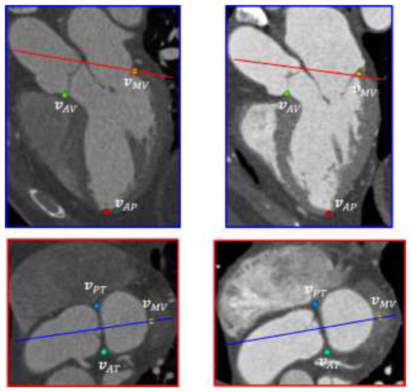
Examples of detected landmarks on two datasets (left and right columns). The colored lines in both planes represent corresponding locations of the other plane.

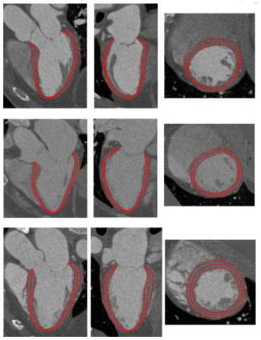
After LV initialization with the detected landmarks, we evaluate our LV segmentation method by 5-fold cross-validation. Both the boundary classifiers and PCA prior are trained and tested with the split datasets by cross-validation. We define two types of segmentation error. One is the error over the whole model E_p2m, which is the common point-to-mesh distance between the segmented mesh ( ${\mathcal{M}}_{\text{seg}}^{\text{endo}}$ or ${\mathcal{M}}_{\text{seg}}^{\text{epi}}$) and the ground-truth mesh ( ${\mathcal{M}}_{\text{truth}}^{\text{endo}}$ or ${\mathcal{M}}_{\text{truth}}^{\text{epi}}$). For every point on a mesh, the closest point on the other mesh (not necessarily mesh vertices) is located and the distance is averaged over the entire mesh. This error is symmetric by averaging the distance computation in both directions. The other error E_p2c is defined only over the boundary contour to evaluate the fitting of this contour. It is also computed in both directions as the point-to-contour distance between the contours on the segmented mesh and the ground-truth mesh. For every point on a contour, the closest point on the other contour (not necessarily contour vertices) is located and the distance is averaged over the whole contour. Table 2 lists the results of E_p2m for the segmentation of LV endocardium and epicardium. After LV initialization with the transformation from the landmarks, the mean of E_p2m for LV endocardium (3.29mm) is slightly higher than epicardium (3.19mm). But after vertex displacement by learned classifiers, both E_p2m are reduced significantly to 1.00mm and 1.11mm. Also, the standard deviations of E_p2m decreases (from 0.84 to 0.43mm for LV endocardium and from 0.77 to 0.50mm), which indicates that the errors tend to be closer to the mean E_p2m. Finally, the PCA prior further decreases the mean and standard deviations of E_p2m for both LV endocardium and epicardium, showing that the PCA prior for constraining the deformation increments is able to reduce the errors caused by misclassification in case of weak boundaries. Table 3 lists the results of E_p2c. The boundary contour deviates largely from the ground-truth (4.31mm). The error reduces to 3.82mm if the boundary vertices are only displaced in the normal direction. As a comparison, the error reduced by almost 1mm to 2.90mm with the displacement of vertices in the direction of b⃗. Finally, the error is further reduced to 2.79mm by enforcing the PCA prior on the displacements. Fig. 9 shows three examples of segmentation results.

Table 2.

The mean and standard deviation (±) of segmentation errors for the whole model E_p2m in different steps (in millimeters). Note E_p2m is computed from all vertices in the model.

Step	LV Endocardium	LV Epicardium
After LV Initialization	3.29±0.84	3.19±0.77
After vertex displacement	1.04±0.43	1.11±0.50
After PCA prior	1.00±0.39	1.06±0.43

Table 3.

The mean and standard deviation (±) of segmentation errors for the boundary contour E_p2c in different steps (in millimeters). Note E_p2c is computed from only the vertices on the boundary contour.

Step	Boundary Contour
After LV Initialization	4.31±0.98
After vertex displacement without movement along b⃗	3.82±1.03
After vertex displacement with movement along b⃗	2.90±0.55

Fig. 9.

Examples of segmented LV endocardial, midcardial, and epicardial surfaces on three datasets. Each row shows views of one dataset from horizontal long axis, vertical long axis, and short axis.

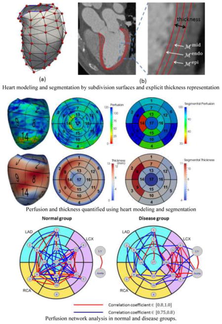
To quantify perfusion and thickness from the LV segmentation, we show an interesting example in Fig. 10. The perfusion in this case is computed as the average image intensity between $\mathit{x}-\frac{\theta }{2}\overrightarrow{\mathit{n}}$ and $\mathit{x}+\frac{\theta }{2}\overrightarrow{\mathit{n}}$ for any point x on the mesh, where thickness θ is readily available in our model. Mapping the measurements at all points on the AHA 17-segment model, the segmental perfusion and thickness are calculated as all measurements within each segment. Clearly, two segments (#13: apical anterior and #14: apical septal) manifest lower image intensity suggesting the contrast concentration in both segments is low. In comparison, the thickness in corresponding regions also clearly decreases, using neighboring regions in the same segment as a reference. It suggests that hypoperfusion may have caused wall thinning as a consequence of myocardial infarction.

Fig. 10.

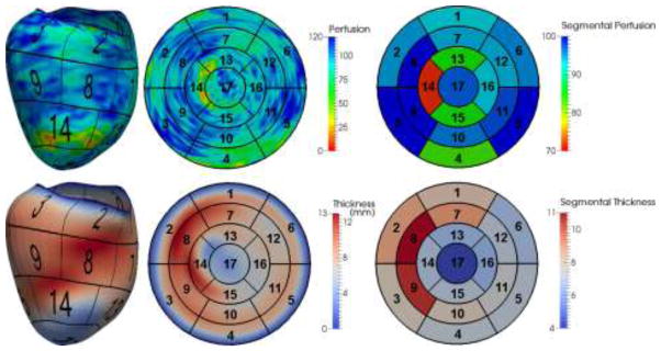
An example of perfusion and thickness quantified using our model. The color maps show the measurement at each point on the mesh, mapped values on the AHA 17-segment model and measurements averaged within each segment.

4.2 Perfusion Network Analysis

Using the segmental perfusions, the aortic and LV blood pool perfusions, the correlation matrix (P) is computed in normal (n=84) and diseased groups (n=56). Fig. 11 shows distributions of the correlation coefficients on each group, where coefficients on the diagonal are always one and thus ignored. The perfusions in different regions are positively correlated, with similar correlation coefficients ranges for the normal (from 0.36 to 0.90) and disease group (from 0.27 to 0.93). However, we find highly correlated region pairs (with correlation coefficients greater than 0.75) in the disease group differ significantly compared to the normal group using perfusion network analysis, as shown in Fig. 12. The interconnections in the normal group is more evenly distributed than the disease group, where the interconnections are weakened in LAD and RCA territories, but elevated in LCX territories. The potential reason for this difference may be because of the reduction of coronary flow, the flow compensation mechanism by collateral vessels or the remodeling of the microcirculation in myocardial wall. Furthermore, there is a strong correlation between intensities in LV blood pool and aorta in both groups. However, their interconnections to the myocardial segments are more prominent in the disease than in the normal group. Quantitatively, we define intra-territory and inter-territory connection strengths as the average correlation coefficient within every pair of segments within one territory and between two territories. Table 4 lists the connection strengths, which confirms our findings. In addition, the segment #4 does not have large correlation to any other segment in both groups, which may be caused by the beam hardening artifact, which is unrelated to myocardial perfusion.

Fig. 11.

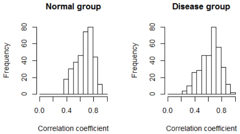
The distribution of correlation coefficients in normal and disease groups.

Fig. 12.

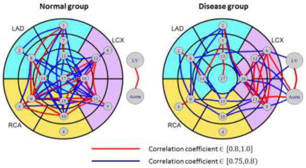
Perfusion network analysis in normal and disease groups.

Table 4.

Intra-segment and inter-segment connection strengths in normal (top in each cell) and disease groups (bottom in each cell). Red indicates increase, while blue indicates decrease.

Normal	LAD	LCX	RCA	LV	Aorta
Disease
LAD	0.69	-	-	-	-
	0.65
LCX	0.67	0.76	-	-	-
	0.60	0.84
RCA	0.66	0.69	0.70	-	-
	0.54	0.65	0.70
LV	0.49	0.47	0.48	-	-
	0.47	0.72	0.61
Aorta	0.60	0.66	0.62	0.85	-
	0.53	0.81	0.65	0.93

4.3 Perfusion Prediction Analysis

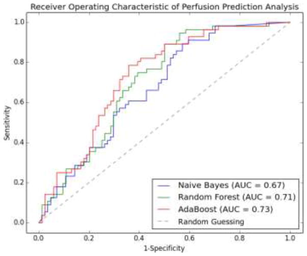
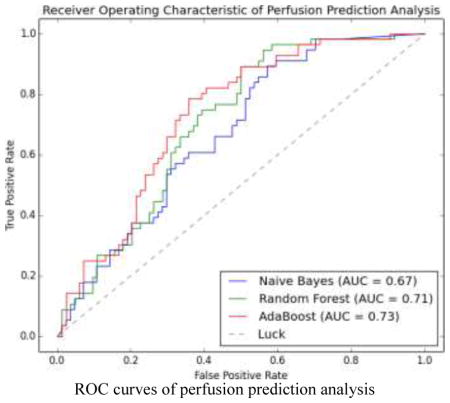
We evaluated three learning methods using leave-one-out cross validation. For any sample (any image in the dataset of 140 images) to be predicted, a classifier was trained on the remaining samples until all samples were predicted. Therefore, a total of 140 classifiers were trained for this purpose. The probability of a sample being positive was calculated by the corresponding classifier and the receiver operating characteristics (ROC) was formed together with the ground-truth label of the sample. Fig. 13 shows the ROC curves for Naive Bayes (NB), Random Forest (RF), and AdaBoost (ADA), where AdaBoost performs slightly better than two other classifiers in terms of the area under the curve (AUC). In addition, AdaBoost is superior in all four metrics of specificity (SPE), accuracy (ACC), positive predictive value (PPV), and negative predictive value (NPV) at the level of sensitivity (SEN) equal to 0.6, 0.7 and 0.8 as shown in Table 5. The best accuracy achieved by the AdaBoost classifier is 0.70, with the associated SEN, SPE, PPV, NPV being 0.79, 0.64, 0.59, and 0.82, respectively. To assess the contributions of different sets of features in the prediction analysis, we train three new AdaBoost classifiers, with only NPI, TPR, or MWT feature. Fig. 14 shows the ROC curves of these three classifiers as compared to the classifier trained with all three features. It is clear that the classifier with three features performs better than the one with only one feature in terms of the AUC. Interestingly, the NPI feature is more effective in the high sensitive end of the curve by improving the specificity. In contrast, the TPR and MWT features improve the sensitivity when the specificity is intermediate or high. It is noted that the ROC curves for TPR and MWT have similar trends, which indicates that their contributions to the prediction performance are comparable and only one may be needed in practice. Although both NPI and TPR are computed from image intensities, their contributions are different and complementary. We thus indirectly show the subtlety of how CT image intensities should be used to evaluate myocardial perfusion. On the other hand, MWT features indeed show certain prediction ability, in spite of being purely geometric.

Fig. 13.

ROC curves of perfusion prediction analysis using Naive Bayes, Random Forest and AdaBoost.

Table 5.

Classification performance at three levels of sensitivity.

SEN	Classifier	SPE	ACC	PPV	NPV
0.6	NB	0.64	0.63	0.53	0.71
	RF	0.69	0.65	0.56	0.72
	ADA	0.71	0.67	0.58	0.73
0.7	NB	0.51	0.59	0.49	0.72
	RF	0.62	0.65	0.55	0.76
	ADA	0.68	0.69	0.59	0.77
0.8	NB	0.48	0.61	0.50	0.78
	RF	0.51	0.63	0.52	0.79
	ADA	0.61	0.68	0.58	0.82

Fig. 14.

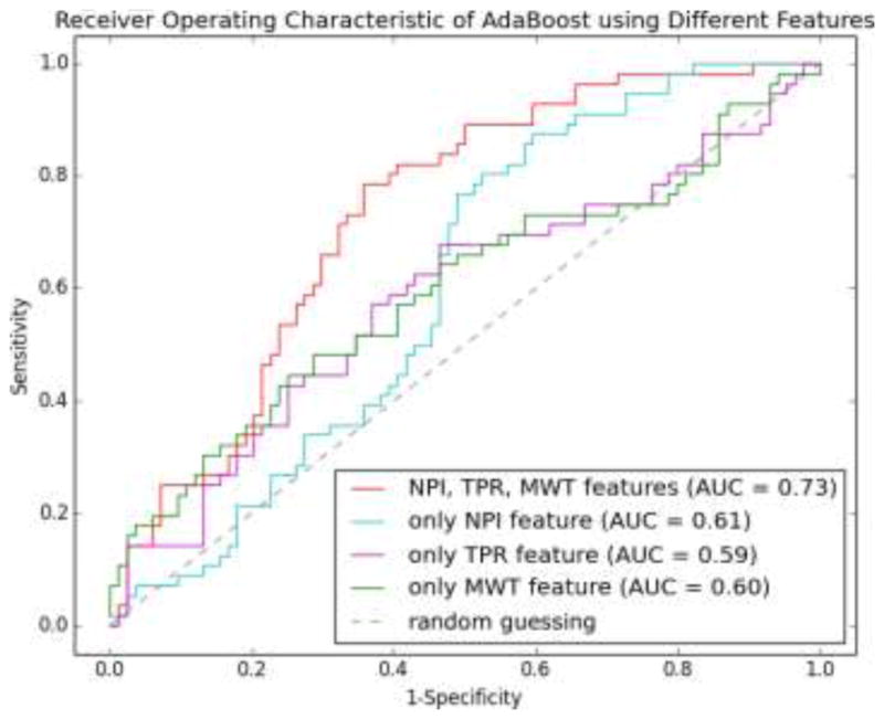
ROC curves of AdaBoost classifiers using different sets of features. The classifier using all three features performs better than that using only one feature.

5. Discussion and Conclusion

In this paper, we have developed a novel framework in order to analyze myocardial perfusion using standard cardiac CTA images acquired at rest. The system includes a model-based segmentation method for delineating the left ventricle surfaces automatically. The surfaces are modeled by subdivision surfaces, which allow us to reduce the number of control vertices and still maintaining the smoothness. The explicit thickness specification of the myocardial wall in our model leads to a compact and coupled representation for both endocardium and epicardium. A template LV model was reconstructed from one image. The model is adapted to a target image by first applying affine transformation with automatically detected five anatomical landmarks and then displacing the control vertices and varying the thicknesses driven by a trained AdaBoost classifier. To be more reliable on weak boundaries, we propose a PCA-based prior to regularize the vertex displacement and thickness variation. Although bias may be created towards the image for template reconstruction, such bias will be minimized by landmark-based affine transformation and boundary alignment by vertex displacement. The evaluation using cross-validation has shown that the overall segmentation error is 1.00±0.39 mm for endocardium and 1.06±0.43 mm for epicardium, respectively.

Based on our LV model, two independent types of myocardial perfusion analysis have been performed, based on the QCA reference standard. One is exploratory, which we propose a new concept of “perfusion network analysis” to discover the relationship between the perfusion intensities among different pairs of myocardial segments defined in AHA 17-segment model. The perfusion network is constructed by considering the segments as nodes and large correlation coefficients as edges. Using the absence and presence of ≥50% stenosis by invasive QCA results, we divide the patients in the normal and disease groups. We find the perfusion network displays different patterns in the two groups, which may be attributed to the impact of disturbing the myocardial perfusion by ischemia or myocardial infarction. It is well known that the metabolic demand and perfusion are not homogenously distributed. Therefore, we expect that the perfusion network exhibits heterogeneity even in normal subjects. Furthermore, this baseline connectivity may be even disturbed by significant obstruction of coronary arteries causing acute ischemia or chronic myocardial infarction. Although our preliminary results are interesting, the findings should be carefully interpreted since our goal in this paper is to provide a new perspective to understand normal and diseased physiology of the heart, especially the relationship of myocardial perfusion among different territories. Future work should be to investigate using dynamic CT perfusion data and larger patient cohort to verify the prevalence and consistency of such difference in myocardial perfusion network. From this, another interesting possibility is to establish the covariance matrix of perfusion values using a population of normal subjects and determine whether perfusion in a new patient is abnormal by computing the Mahalanobis distance. In addition, other techniques used in the brain network analysis can be explored to build the network weights beyond correlation, e.g. sparse inverse correlation (Liu et al., 2009), mutual information, etc. (Zhou et al., 2009).

The other analysis is confirmatory which aims to assess the ability to predict whether a patient has significant coronary stenosis by QCA by quantification of perfusion and thickness using noninvasive CTA images acquired at rest. By extracting three features, namely, normalized perfusion intensity, transmural perfusion ratio, and myocardial wall thickness, we have shown that noninvasive quantification is indeed able to predict the invasive measurement results using standard machine learning techniques. Our experiment shows that a classifier based on AdaBoost is able to obtain a moderate accuracy of 0.7 with sensitivity and specificity equal to 0.79 and 0.64, which is slightly better than Naive Bayes and Random Forest. We also find that the prediction performance benefits by using all three features instead of only one feature. Our results demonstrate that myocardial perfusion quantified on noninvasively acquired CTA images at rest indeed has reasonable predictive ability for information obtained using invasively acquired QCA data. Utility of the prediction analysis in addition to other routine image interpretation tasks on CTA is straightforward with our automatic method. In this paper, we have predicted the existence of significant stenosis by invasive QCA on the patient level. Future work will be to study the reliability of per-vessel prediction using supervised classification techniques, as well as the feasibility of predicting the degree of stenosis severity as a continuous variable or the presence of stenosis at single or multiple locations using supervised regression techniques. In addition, the performance of identifying stenosis visually by CTA has been widely examined using QCA as reference standard. Because the focus of this paper is to show the prediction ability of the automatically quantified perfusion alone, the incremental value of perfusion analysis to visual CTA-based stenosis is not examined but will be our future work. Furthermore, our current work is limited to predict the anatomic significance by invasive QCA. Since QCA is not considered as a reference standard of physiologic significance, our ongoing work is to utilize a reference standard of more hemodynamic relevance, e.g. FFR (Tonino et al., 2009). Finally, our approaches can be also extended to analyze myocardial perfusion under stress and dynamic CT perfusion data, where quantitative measurements of contrast concentration are available. We believe such analysis will improve the prediction ability of coronary artery stenoses, especially those of intermediate grades between 50% and 70%. In summary, we have demonstrated the usefulness of myocardial perfusion analysis from typically-acquired CTA images at rest.

Highlights.

• We proposed a new system the physiologic manifestation of coronary stenoses by assessment of myocardial perfusion from typically acquired CT images at rest.

• We developed an automated segmentation method based on subdivision surfaces and machine learning.

• We performed perfusion network analysis which shows different patterns of connectivity in the normal and disease groups.

• We also performed the analysis of using perfusion and thickness features to predict the outcomes of invasive coronary angiography with accuracy, sensitivity and specificity of 0.70, 0.79 and 0.64, respectively.

References

- Berman DS, Hachamovitch R, Shaw LJ, Friedman JD, Hayes SW, Thomson LEJ, Fieno DS, Germano G, Slomka P, Wong ND, Kang X, Rozanski A. Roles of nuclear cardiology, cardiac computed tomography, and cardiac magnetic resonance: assessment of patients with suspected coronary artery disease. J Nucl Med. 2006;47:74–82. [PubMed] [Google Scholar]
- Blankstein R, Shturman LD, Rogers IS, Rocha-Filho JA, Okada DR, Sarwar A, Soni AV, Bezerra H, Ghoshhajra BB, Petranovic M, Loureiro R, Feuchtner G, Gewirtz H, Hoffmann U, Mamuya WS, Brady TJ, Cury RC. Adenosine-induced stress myocardial perfusion imaging using dual-source cardiac computed tomography. J Am Coll Cardiol. 2009;54:1072–84. doi: 10.1016/j.jacc.2009.06.014. [DOI] [PubMed] [Google Scholar]
- Breiman L. Random Forests. Mach Learn. 2001;45:5–32. doi: 10.1023/A:1010933404324. [DOI] [Google Scholar]
- Buckner RL, Andrews-Hanna JR, Schacter DL. The brain’s default network: anatomy, function, and relevance to disease. Ann N Y Acad Sci. 2008;1124:1–38. doi: 10.1196/annals.1440.011. [DOI] [PubMed] [Google Scholar]
- Budoff MJ, Dowe D, Jollis JG, Gitter M, Sutherland J, Halamert E, Scherer M, Bellinger R, Martin A, Benton R, Delago A, Min JK. Diagnostic performance of 64-multidetector row coronary computed tomographic angiography for evaluation of coronary artery stenosis in individuals without known coronary artery disease: results from the prospective multicenter ACCURACY (Assessment by Coro. J Am Coll Cardiol. 2008;52:1724–32. doi: 10.1016/j.jacc.2008.07.031. [DOI] [PubMed] [Google Scholar]
- Cerqueira MD. Standardized Myocardial Segmentation and Nomenclature for Tomographic Imaging of the Heart: A Statement for Healthcare Professionals From the Cardiac Imaging Committee of the Council on Clinical Cardiology of the American Heart Association. Circulation. 2002;105:539–542. doi: 10.1161/hc0402.102975. [DOI] [PubMed] [Google Scholar]
- Ecabert O, Peters J, Schramm H, Lorenz C, von Berg J, Walker MJ, Vembar M, Olszewski ME, Subramanyan K, Lavi G, Weese J. Automatic model-based segmentation of the heart in CT images. IEEE Trans Med Imaging. 2008;27:1189–201. doi: 10.1109/TMI.2008.918330. [DOI] [PubMed] [Google Scholar]
- Ecabert O, Peters J, Walker MJ, Ivanc T, Lorenz C, von Berg J, Lessick J, Vembar M, Weese J. Segmentation of the heart and great vessels in CT images using a model-based adaptation framework. Med Image Anal. 2011;15:863–76. doi: 10.1016/j.media.2011.06.004. [DOI] [PubMed] [Google Scholar]
- Frangi AF, Niessen WJ, Viergever MA. Three-dimensional modeling for functional analysis of cardiac images: a review. IEEE Trans Med Imaging. 2001;20:2–25. doi: 10.1109/42.906421. [DOI] [PubMed] [Google Scholar]
- George RT, Arbab-Zadeh A, Miller JM, Kitagawa K, Chang HJ, Bluemke DA, Becker L, Yousuf O, Texter J, Lardo AC, Lima JAC. Adenosine stress 64- and 256-row detector computed tomography angiography and perfusion imaging: a pilot study evaluating the transmural extent of perfusion abnormalities to predict atherosclerosis causing myocardial ischemia. Circ Cardiovasc Imaging. 2009;2:174–82. doi: 10.1161/CIRCIMAGING.108.813766. [DOI] [PMC free article] [PubMed] [Google Scholar]
- George RT, Silva C, Cordeiro MAS, DiPaula A, Thompson DR, McCarthy WF, Ichihara T, Lima JAC, Lardo AC. Multidetector computed tomography myocardial perfusion imaging during adenosine stress. J Am Coll Cardiol. 2006;48:153–60. doi: 10.1016/j.jacc.2006.04.014. [DOI] [PubMed] [Google Scholar]
- Gershlick AH, de Belder M, Chambers J, Hackett D, Keal R, Kelion A, Neubauer S, Pennell DJ, Rothman M, Signy M, Wilde P. Role of non-invasive imaging in the management of coronary artery disease: an assessment of likely change over the next 10 years. A report from the British Cardiovascular Society Working Group. Heart. 2007;93:423–31. doi: 10.1136/hrt.2006.108779. [DOI] [PMC free article] [PubMed] [Google Scholar]
- Greicius MD, Krasnow B, Reiss AL, Menon V. Functional connectivity in the resting brain: a network analysis of the default mode hypothesis. Proc Natl Acad Sci U S A. 2003;100:253–8. doi: 10.1073/pnas.0135058100. [DOI] [PMC free article] [PubMed] [Google Scholar]
- Hoogendoorn C, Duchateau N, Sánchez-Quintana D, Whitmarsh T, Sukno FM, De Craene M, Lekadir K, Frangi AF. A high-resolution atlas and statistical model of the human heart from multislice CT. IEEE Trans Med Imaging. 2013;32:28–44. doi: 10.1109/TMI.2012.2230015. [DOI] [PubMed] [Google Scholar]
- Isgum I, Staring M, Rutten A, Prokop M, Viergever MA, van Ginneken B. Multi-atlas-based segmentation with local decision fusion--application to cardiac and aortic segmentation in CT scans. IEEE Trans Med Imaging. 2009;28:1000–10. doi: 10.1109/TMI.2008.2011480. [DOI] [PubMed] [Google Scholar]
- Kachenoura N, Veronesi F, Lodato JA, Corsi C, Mehta R, Newby B, Lang RM, Mor-Avi V. Volumetric quantification of myocardial perfusion using analysis of multi-detector computed tomography 3D datasets. 2009 doi: 10.1007/s00330-009-1552-x. [DOI] [PubMed] [Google Scholar]
- Kang D, Woo J, Slomka PJ, Dey D, Germano G, Jay Kuo C-C. Heart chambers and whole heart segmentation techniques: review. J Electron Imaging. 2012 doi: 10.1117/1.JEI.21.1.010901. [DOI] [Google Scholar]
- Kearns MJ, Vazirani UV. Computational Learning Theory. In: Vitányi P, editor. ACM SIGACT News, Lecture Notes in Computer Science. Springer Berlin Heidelberg; Berlin, Heidelberg: 1995. pp. 43–45. [DOI] [Google Scholar]
- Kirişli HA, Schaap M, Klein S, Papadopoulou SL, Bonardi M, Chen CH, Weustink AC, Mollet NR, Vonken EJ, van der Geest RJ, van Walsum T, Niessen WJ. Evaluation of a multi-atlas based method for segmentation of cardiac CTA data: a large-scale, multicenter, and multivendor study. Med Phys. 2010;37:6279. doi: 10.1118/1.3512795. [DOI] [PubMed] [Google Scholar]
- Ko BS, Cameron JD, Meredith IT, Leung M, Antonis PR, Nasis A, Crossett M, Hope SA, Lehman SJ, Troupis J, DeFrance T, Seneviratne SK. Computed tomography stress myocardial perfusion imaging in patients considered for revascularization: a comparison with fractional flow reserve. Eur Heart J. 2012;33:67–77. doi: 10.1093/eurheartj/ehr268. [DOI] [PubMed] [Google Scholar]
- Liu J, Ji S, Ye J. SLEP: Sparse Learning with Efficient Projections 2009 [Google Scholar]
- Lloyd-Jones D, Adams RJ, Brown TM, Carnethon M, Dai S, De Simone G, Ferguson TB, Ford E, Furie K, Gillespie C, Go A, Greenlund K, Haase N, Hailpern S, Ho PM, Howard V, Kissela B, Kittner S, Lackland D, Lisabeth L, Marelli A, McDermott MM, Meigs J, Mozaffarian D, Mussolino M, Nichol G, Roger VL, Rosamond W, Sacco R, Sorlie P, Stafford R, Thom T, Wasserthiel-Smoller S, Wong ND, Wylie-Rosett J. Heart disease and stroke statistics--2010 update: a report from the American Heart Association. Circulation. 2010;121:e46–e215. doi: 10.1161/CIRCULATIONAHA.109.192667. [DOI] [PubMed] [Google Scholar]
- Loop C. Smooth Subdivision Surfaces Based on Triangles. University of Utah; 1987. [Google Scholar]
- Lorenz C, von Berg J. A comprehensive shape model of the heart. Med Image Anal. 2006;10:657–70. doi: 10.1016/j.media.2006.03.004. [DOI] [PubMed] [Google Scholar]
- Mehra VC, Valdiviezo C, Arbab-Zadeh A, Ko BS, Seneviratne SK, Cerci R, Lima JAC, George RT. A stepwise approach to the visual interpretation of CT-based myocardial perfusion. J Cardiovasc Comput Tomogr. 2011;5:357–69. doi: 10.1016/j.jcct.2011.10.010. [DOI] [PubMed] [Google Scholar]
- Min JK, Shaw LJ, Berman DS. The present state of coronary computed tomography angiography a process in evolution. J Am Coll Cardiol. 2010;55:957–65. doi: 10.1016/j.jacc.2009.08.087. [DOI] [PubMed] [Google Scholar]
- Pijls NH, De Bruyne B, Peels K, Van Der Voort PH, Bonnier HJ, Bartunek J, Koolen JJ, Koolen JJ. Measurement of fractional flow reserve to assess the functional severity of coronary-artery stenoses. N Engl J Med. 1996;334:1703–1708. doi: 10.1056/NEJM199606273342604. [DOI] [PubMed] [Google Scholar]
- Reiber JHC, Kooijman CJ, Slager CJ, Gerbrands JJ, Schuurbiers JCH, Boer A, Den Wijns W, Serruys PW, Hugenholtz PG. Coronary Artery Dimensions from Cineangiograms-Methodology and Validation of a Computer-Assisted Analysis Procedure. IEEE Trans Med Imaging. 1984;3 doi: 10.1109/TMI.1984.4307669. [DOI] [PubMed] [Google Scholar]
- Tamarappoo BK, Dey D, Nakazato R, Shmilovich H, Smith T, Cheng VY, Thomson LEJ, Hayes SW, Friedman JD, Germano G, Slomka PJ, Berman DS. Comparison of the extent and severity of myocardial perfusion defects measured by CT coronary angiography and SPECT myocardial perfusion imaging. JACC Cardiovasc Imaging. 2010;3:1010–9. doi: 10.1016/j.jcmg.2010.07.011. [DOI] [PubMed] [Google Scholar]
- Taylor CA, Fonte TA, Min JK. Computational fluid dynamics applied to cardiac computed tomography for noninvasive quantification of fractional flow reserve: scientific basis. J Am Coll Cardiol. 2013;61:2233–41. doi: 10.1016/j.jacc.2012.11.083. [DOI] [PubMed] [Google Scholar]
- Techasith T, Cury RC. Stress myocardial CT perfusion: an update and future perspective. JACC Cardiovasc Imaging. 2011;4:905–16. doi: 10.1016/j.jcmg.2011.04.017. [DOI] [PubMed] [Google Scholar]
- Tonino PAL, De Bruyne B, Pijls NHJ, Siebert U, Ikeno F, van’t Veer M, Klauss V, Manoharan G, Engstrøm T, Oldroyd KG, Ver Lee PN, MacCarthy PA, Fearon WF. Fractional flow reserve versus angiography for guiding percutaneous coronary intervention. N Engl J Med. 2009;360:213–24. doi: 10.1056/NEJMoa0807611. [DOI] [PubMed] [Google Scholar]
- Van Rikxoort EM, Isgum I, Arzhaeva Y, Staring M, Klein S, Viergever MA, Pluim JPW, van Ginneken B. Adaptive local multi-atlas segmentation: application to the heart and the caudate nucleus. Med Image Anal. 2010;14:39–49. doi: 10.1016/j.media.2009.10.001. [DOI] [PubMed] [Google Scholar]
- Zheng Y, Barbu A, Georgescu B, Scheuering M, Comaniciu D. Four-chamber heart modeling and automatic segmentation for 3-D cardiac CT volumes using marginal space learning and steerable features. IEEE Trans Med Imaging. 2008;27:1668–81. doi: 10.1109/TMI.2008.2004421. [DOI] [PubMed] [Google Scholar]
- Zhou D, Thompson WK, Siegle G. MATLAB toolbox for functional connectivity. Neuroimage. 2009;47:1590–607. doi: 10.1016/j.neuroimage.2009.05.089. [DOI] [PMC free article] [PubMed] [Google Scholar]