

Abstract
Dynamic contrast-enhanced magnetic resonance imaging (DCE-MRI) enables the quantification of contrast leakage from the vascular tissue by using pharmacokinetic (PK) models. Such quantitative analysis of DCE-MRI data provides physiological parameters that are able to provide information of tumor pathophysiology and therapeutic outcome. Several assumptive PK models have been proposed to characterize microcirculation in the tumoral tissue. In this paper, we present a comparative study between the well-known extended Tofts model (ETM) and the more recent gamma capillary transit time (GCTT) model, with the latter showing initial promising results in the literature. To enhance the GCTT imaging biomarkers, we introduce a novel method for segmenting the tumor area into subregions according to their vascular heterogeneity characteristics. A cohort of 11 patients diagnosed with glioblastoma multiforme with known therapeutic outcome was used to assess the predictive value of both models in terms of correctly classifying responders and nonresponders based on only one DCE-MRI examination. The results indicate that GCTT model’s PK parameters perform better than those of ETM, while the segmentation of the tumor regions of interest based on vascular heterogeneity further enhances the discriminatory power of the GCTT model.
Keywords: DCE-MRI, pharmacokinetic modeling, perfusion imaging, brain tumor, imaging biomarkers
Introduction
Magnetic resonance imaging (MRI) is the most commonly used medical imaging technique to demonstrate tumor morphology and the relationships between malignant lesions and the neighboring structures. MRI also provides relevant clinical information for clinical management and surgical planning. In recent years, sequential sets of MRI data and the development of small molecular weight paramagnetic contrast agents have had a major impact in the assessment and monitoring of tumor treatment response.1
The blood–brain barrier (BBB)2 is a membrane that separates the parenchyma of the central nervous system from the blood. It consists of endothelial cells interconnected by tight junctions that cause a selective permeability based on molecular weight and osmotic characteristics. In pathologies such tumors,3 multiple sclerosis,4 and acute ischemic strokes,5 the BBB is disrupted by various mechanisms. The BBB disruption is reflected by, for example, MRI contrast enhancement in pathological areas.
Dynamic contrast-enhanced magnetic resonance imaging (DCE-MRI) is a useful imaging technique for assessing the BBB leakage; it is based on the extravasation of the contrast agent (CA) from arteries to the parenchyma, which leads to decreased longitudinal relaxation time and therefore increased MRI signal intensity. It relies on fast T1-weighted MRI sequences obtained before, during, and after the intravenous administration of a gadolinium (Gd)-based CA.
There are several models for the quantification of DCE-MRI data that can be applied in many anatomical areas such as brain, prostate, and breast tissue, aiming to extract tissue physiological parameters. These models provide independent markers of angiogenic activity, and therefore act as diagnostic and prognostic indicators in a broad range of tumor types. A number of physiological parameters of vascularization coming from pharmacokinetic (PK) models play an important role in quantitatively assessing tumor angiogenesis within a region. Neovascularity and leaky vessels are associated with higher ktrans (volume transfer constant between plasma and EES) values, while response to therapy has been correlated with a drop in ktrans values between imaging sessions.6 The results can be combined with other quantitative measures such as T2* perfusion7 in brain and H215 O-PET8 in body imaging for the evaluation of treatment response. In this paper, we study the applicability of PK models for the early characterization of therapy response in glioblastoma multiforme (GBM) patients and also present a novel framework for enhancing the imaging biomarkers by pre-segmenting the tumor region of interest (ROI) into subregions according to vascular heterogeneity metrics.
Methods
MRI acquisition protocol
All MRI acquisitions were performed on a 3-T Philips scanner. Prior to the CA injection, two acquisitions were made for the variable flip angle (VFA) data using flip angles (FA) of 5° and 15°, repetition time (TR) of 10 ms, and echo time (TE) of 2 ms. DCE-MRI data were acquired using fast three-dimensional spoiled gradient echo (SPGR) with TR 3.6 ms, TE 1.75 ms, and FA 6°. The dimensions of the image was 192 × 192 voxels with 36 slices and 50 time points for DCE-MRI protocol, temporal resolution 6 s, and the size of one voxel 1.15 × 1.15 × 2.99 mm. The type of CA that was used was Dotarem, and the quantity was 0.1 mmol/kg of body weight.
Preprocessing
All datasets (both DCE-MRI and VFA) were co-registered to the arterial phase [maximum signal-to-noise ratio (SNR)] of the DCE-MRI, and a temporal smoothing algorithm was subsequently used to remove the intrinsic noise of the MRI signal. Due to the large discrepancies in the values of arterial concentrations among different subjects, we used a theoretical arterial input function (AIF) for all subjects. To this end, biexponential decay was assumed to describe the plasma concentration using values from earlier work.9
Estimation of contrast agent concentration
To proceed to the quantification of CA kinetics from signal intensities (SIs), the concentration of CA should be determined at each time point of the dynamic scan; possibly the most crucial step. A first approach is to assume that the CA concentration is proportional to the change in SI. However, when CA concentrations are high, the relationship between concentration and SI becomes nonlinear10 and the previous approximation may lead to significant errors.
There are several techniques for measuring changes in T1 due to CA presence, such as inversion recovery,11–13 Look-Locker,14,15 and VFA.3,16–18 The VFA method was chosen in our work because of the good SNR and reduced acquisition times.
The CA concentration is related to the change in relaxation time via the following formula:
| (1) |
where r1 is the longitudinal relaxivity of the CA, T10 is the longitudinal relaxation time without CA, and T1(t) is the longitudinal relaxation at time t after the injection.
The MRI signal S1 acquired with TE ≪ T2* is given by the following equation:
| (2) |
where S0 is the relaxed signal for a 90° pulse when TR ≫ T1, αf is the flip angle, and TR is the repetition time. Substituting in Equation (2) the measurements acquired from the VFAs data and solving the nonlinear problem per voxel, the vector [S0, T10] is calculated.
Substituting in Equation (2)S1 with S(t) (the SI in DCE-MRI data) and αf with a (flip angle that was used in DCE-MRI protocol), and solving for T1, the time course of the longitudinal relaxation time can be calculated from Equation (3).
| (3) |
The overall procedure is depicted in Figure 1, where using the VFAs data, vector [S0, T10] is estimated using Equation (2). Afterward, using DCE-MRI data, the time course of the longitudinal relaxation time (T1(t)) is calculated by Equation (3). Substituting the pre-contrast relaxation time (T10) and the time course of the longitudinal relaxation time (T1(t)) in Equation (1); the CA concentration is calculated.
Figure 1.
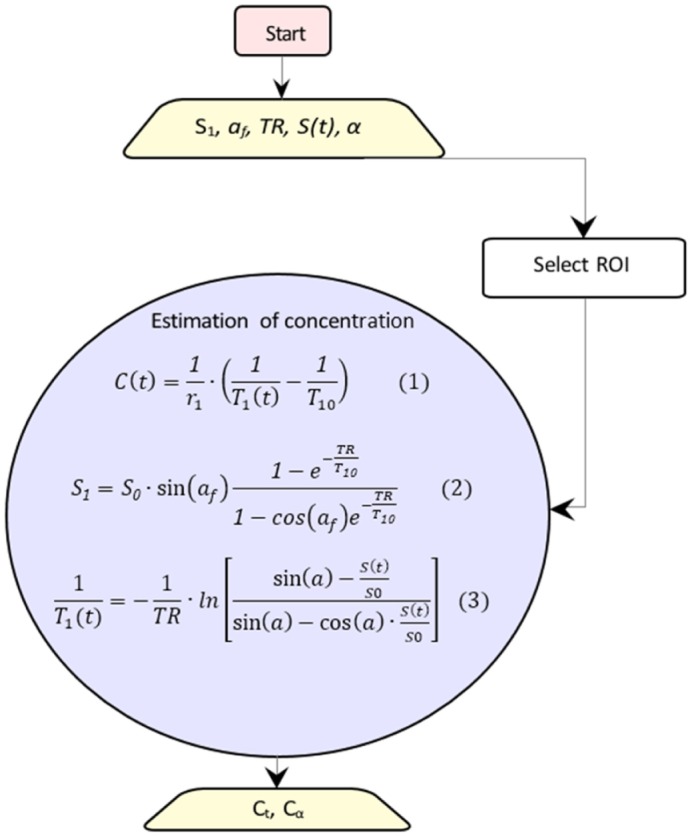
Schematic diagram for converting signal intensity into concentrations. The rectangle shows the start point, the trapeziums show the parameters, and the circle includes the equations to be solved.
Impulse response function
Using systems theory and assuming that biological tissues are linear, time-invariant systems, tracer kinetics can be described by the impulse response function (IRF),19 which incorporates the physiological parameters at each voxel. This way, the tissue concentration is given by Equation (4):
| (4) |
where IRF(t) = IRFv(t) + IRFp(t), with IRFv the vascular impulse response function and IRFp the parenchymal impulse response function, F is the flow, Ct is the concentration in the tissue, Cα is the concentration in the arterial blood (AIF), and ⊗ represents convolution.
Tofts and extended Tofts model
The most commonly used model in literature is the Tofts model (TM),20 which is a single-compartment model in which CA diffuses from an external vascular space into a well-mixed tissue compartment. Tofts et al assumed that when CA is injected to the bloodstream, it will pass the disrupted blood vessel endothelium and move to the extravascular extracellular space (EES) with a rate proportional to the difference of CA concentration between the plasma (Cα(t)) and the EES space (Ct(t)):
| (5) |
Using the convolution theorem, the solution of Equation (5) is given by the following formula:
| (6) |
with IRFv(t) = 0 and IRF . In the above equations, ktrans represents the volume transfer constant from the plasma space to EES, ve is the volume of EES, and kep=ktrans/ve is the transfer constant from EES to the plasma space. The negligible plasma volume assumption of TM is invalid for several tissue types, especially for brain tumors, which might lead to significant errors.
Tofts et al extended the original model by introducing the vascular term as an external compartment. The result was to separate the enhancement caused by contrast leakage from that caused by intravascular contrast. The extended Tofts model (ETM)21 is described by the following equation:
| (7) |
where IRFv(t) = vp·δ(t)/F and IRF , and vp is the volume of vascular space. Given that Ct(t) and Ca(t) are known by converting the tissue and the artery SIs, respectively, and using Equation (7), the vector [ktrans, kep, vp] is estimated per voxel. The weak point of these models is that ktrans can be interpreted either as plasma flow in flow-limited cases or as tissue permeability in permeability-limited cases, but does not allow separate estimation of these two independent parameters. Moreover, TM can provide accurate PK parameters if and only if tissue is weakly vascularized, while ETM is also accurate in highly perfused tissues.22
Gamma capillary transit time
The gamma capillary transit time (GCTT) model23 unifies four models: TM,20 ETM,21 the two-compartment exchange (2CX) model,24 and the adiabatic tissue homogeneity (ATH) model.25 A major drawback of the aforementioned models is that every voxel is treated as a single capillary tissue unit with a single capillary transit time. The distributed capillary adiabatic tissue homogeneity (DCATH) model26 overcame this drawback by assuming a statistical distribution (normal, corrected normal, and skewed) of the transit times in the parenchyma and vascular IRFs. However, the DCATH model failed in the sense that certain results did not correspond to realistic values (eg, negative transit times) and the model could not provide closed-form solutions.23
The GCTT model overcame the limitations of the DCATH model by assuming that capillary transit times are governed by the gamma distribution. This way, each voxel is assumed to have different characteristics that are described by the parameter α−1, which is defined as the width of the distribution of the capillary transit times within a tissue voxel, and actually expresses the heterogeneity of tissue microcirculation and microvasculature.19,23 Depending on this para meter, IRF is adapted to the specific properties of the tissue voxel. Mathematically, the parameter α−1 is expressed by the following equation:
| (8) |
where τ is the scale parameter of the gamma distribution, and tc is the capillary transit time.
The vascular and parenchymal components of the IRF in the GCTT model are given by the following equations:
| (9) |
| (10) |
where D(u) is the gamma distribution of capillary transit times, E is the extraction fraction, which indicates the fraction of CA that is extracted from vp into vt in a single capillary time, γ is the upper incomplete gamma function, and kep is the CA transfer rate from EES to the vascular space. Replacing Equations (9) and (10) in Equation (4), the formula for the GCTT model can be derived as:
| (11) |
As in ETM, Ct(t) and Cα(t) are computed by converting the tissue and the artery SIs, respectively, and then estimating using Equation (11) the vector [F, E, kep, τ, α−1] per voxel. As was mentioned earlier, the GCTT model converges to preexisting models in certain limits of its parameters, as shown in Table 1.
Table 1.
GCTT convergence to other models.
| CONDITION | CONVERGENCE |
|---|---|
| α−1→0 | IRFATH→ IRFGCTT |
| α−1→1 | IRF2cx→IRFGCTT |
| α−1→1, τ→ε | IRFETK→IRFGCTT |
| α−1→1, τ→0 | IRFTK →IRFGCTT |
Heterogeneity tumor region segmentation based on 0−1
In order to enhance the application of the GCTT model in real clinical data, a preprocessing step is proposed by exploiting the α−1 parameter. For this purpose, the MR image of the tumor was segmented based on each voxel’s α−1 value, in order to separate tumor into subregions of similar vascular heterogeneity characteristics. After extensive experimentation and observation of the α−1 histogram characteristics in the tumor ROIs, a four-subregion segmentation scheme was proposed, as shown in Figure 2. It was observed that, in most of the cases, the histogram distributions of the α−1 parameter include three characteristic peaks and a plateau in the same value intervals. The α−1 boundary values were determined empirically based on the average histogram profile. The first subregion consists of the first peak, the second subregion consists of the linear histogram part, the third subregion consists of the second peak, and the fourth subregion consists of the third peak. Provided that the average profile is similar in future studies, it is possible to use the same values and test by other researchers.
Figure 2.
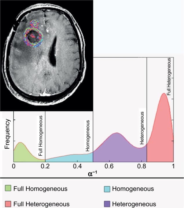
Proposed methodology for separating the tumor image area into four subregions based on the vascular heterogeneity characteristics (α−1). This way, in each subregion as well as in the whole tumor region, the value of all PK GCTT parameters can be assessed separately.
The different subregions are defined as follows:
“Full Homogeneous” subregion: when α−1 ∈ (0,0.2] – in tables of results referred to as 1;
“Homogeneous” subregion: when α−1 ∈ (0.2,0.5] – in tables of results referred to as 2;
“Heterogeneous” subregion: when α−1 ∈ (0.5,0.85] – in tables of results referred to as 3;
“Full Heterogeneous” subregion: when α−1 ∈ (0.85,1) – in tables of results referred to as 4.
This segmentation comprises a new framework which in essence divides each tumor image region into four subregions of differing homogeneity as given by the GCTT model. For each subregion, the PK parameters were collected, and the classification results for the two groups of patients were reported. For completeness, in the comparative study the results in the entire tumor region (“All regions” – in tables of results referred to as 0) were also computed in order to test whether the proposed heterogeneity segmentation framework can add value to the strength of the PK GCTT candidate imaging biomarkers.
Implementation of the models
Figure 3 presents the workflow for the conversion of concentrations to PK parameters. The PK parameters were calculated per voxel via nonlinear least squares problems†, by solving Equation (7) for ETM and Equation (11) for the GCTT model.
Figure 3.

Workflow for calculation of PK parameters. The rectangles show the start and end points, the trapeziums show the extracted PK parameters, and the ellipsoids include the equations to be solved.
In ETM, all parameters were assumed positive, and the initial values of ktrans, kep, and vp were 0.001 (min−1), 0.009 (min−1), and 0.01 (none), respectively.
In GCTT, all parameters were assumed positive and the initial values of F, E, kep, τ, and α−1 were 0.002 (min−1), 0.5 (none), 0.009 (min−1), 1.5 (s), and 0.5 (none), respectively. In the last step, the additional parameters (ktrans, PS, tc, and vp) were calculated by the following equations:
| (12) |
| (13) |
| (14) |
| (15) |
where PS is the permeability surface area product per unit mass of tissue and Hct is the hematocrit (reference value 0.45).
Clinical question for assessing and comparing the PK models
We retrospectively analyzed data from 11 patients (anonymized) diagnosed with GBM from University Hospital of Leuven at a time point before definite diagnosis regarding the therapy outcome. As shown in Table 2, each patient belonged in one of the following three categories: response, immune reaction, and progression, depending on the actual final outcome. Regarding treatment outcome, patients in the first two categories exhibited similar characteristics; thus for testing the discriminatory power of the PK models in this work, we divided patients into two groups: “Response” and “Non-Response”, as shown in Table 2. This decision mainly reflects the most important aspect of this work, ie, to use PK imaging biomarkers for assisting the clinician to early assess the treatment outcome and better manage the therapeutic alternatives.
Table 2.
Clinical cases.
| PATIENT | OUTCOME | GROUP |
|---|---|---|
| P1 | Immune reaction | Response |
| P2 | Immune reaction | Response |
| P3 | Response | Response |
| P4 | Response | Response |
| P5 | Progression | Non-Response |
| P6 | Progression | Non-Response |
| P7 | Progression | Non-Response |
| P8 | Progression | Non-Response |
| P9 | Progression | Non-Response |
| P10 | Progression | Non-Response |
| P11 | Progression | Non-Response |
The data in this study are part of a larger longitudinal imaging study in which patients with GBM treated with immune therapy receive monthly an extensive MRI exam. The institutional review board of the University Hospitals Leuven approved this study and informed consent of every patient was obtained before participation. This was done in order to characterize the temporal pattern on imaging in patients treated with a novel therapy and, secondly, in case an immune reaction was expected, to be able to characterize this with advanced MRI. Clinical outcome of the therapy is thus based on imaging follow-up and clinical examination. The standard imaging guidelines were used to define progression, response, and immune reaction, as defined in the Response Assessment in Neuro-Oncology (RANO) criteria.27 These criteria are currently defined as the standard clinical guidelines and count as good clinical practice. Performing histopathological examination obtained by biopsy or craniotomy at every time point in every patient is unethical. For this reason, no histological information was available in our study.
For each subject, an expert radiologist annotated the ROI of the tumor. The PK parameters were calculated per voxel, and regions with parameters out of bounds or with insufficient goodness of fitness (R2) were excluded. The focus of our work was to define which imaging biomarkers could better predict outcome before definite diagnosis in the two groups of patients with only one imaging study available.
Statistical analysis
An exploratory histogram analysis, using the derived PK parameter maps from the ROIs, was performed, yielding several metrics including the minimum, maximum, mean, standard deviation, median, skewness, kurtosis, variance, as well as the 5%, 30%, 70%, and 95% percentiles for each parameter. A Kruskal–Wallis test28 was applied to a total of 588 parameters (49 PK parameters multiplied by 12 histogram metrics) to investigate the differences between responders and nonresponders in terms of the histogram metrics. The estimated P-values were declared statistically significant only at the 1% significance level. Because of the small sample size, the estimation of the predictive power of each parameter relied on the leave-one-out cross validation (LOO-CV). For every single parameter in the dataset, a LOO-CV took place in which each sample acted as a validation set and the remaining samples were used for training. The aggregated predictive probabilities of each parameter over the entire dataset composed a new set for further analysis. The receiver operator characteristic (ROC) curves were then computed and the corresponding areas under the receiving operating curves (AUCs) were calculated to assess the performance of each parameter in predicting the responsiveness of the treatment accurately. Sensitivity, specificity, negative and positive predictive values, accuracy, the confusion matrix, and the optimal cutoff value of all ROC curves were calculated. The confusion matrix reports the number of true positive (TP), true negative (TN), false positive (FP), and false negative (FN).
All possible linear regression model combinations were generated from the parameters having a P-value <1%, and a model selection framework was intended to select the “best” model that differentiated the two groups. This framework relied on a wrapper approach equipped with parameter(s) selection criteria based on the small-sample corrected Akaike information criterion (AICc).29 AICc was selected instead of the basic AIC30 because the former is strongly recommended in case of having a small cohort for analysis.31 Using wrapper techniques, all possible univariate and multivariate models were first generated, fitted by a regression analysis function, and, based on their AICc value, the optimal model (ie, yielding the lowest AICc) was finally selected.
For the purposes of the analysis, in-house software was written in R32 to fit a linear model of the form “y ~ x1 + x2,…, + xn”, where y is the dependent variable (ie, responders vs nonresponders), and x1, x2,…,xn are the explanatory variables or the parameters derived from the histogram analysis otherwise. The packages “pROC”33 and “glmulti”34 were used for computing the ROC curves, their relative statistical measurements, and the optimal model, respectively. For illustrative purposes, a graphical summary of the analysis was also obtained, containing information about the AICc profile of each model and the estimated importance of each parameter computed as the sum of the relative evidence weights of all models in which the specific parameter appears.
Alternatively, a Lasso regularized generalized linear model, using R package “glmnet”,35 was applied to the entire dataset comprised of 588 parameters. A LOO-CV was performed first to calculate the optimum tuning parameter lambda (λ) referring to the lowest CV error. The optimum lambda was used for fitting the model to the data and the resulting fitted model was then added to R function “predict”, to return the coefficients of the best model (nonzero coefficients).
Results
Parameters with P-values <1% are summarized in Table 3. The name of each parameter is composed by four parts: 1) the applied PK model (ie, GCTT or ETM as described previously), 2) the computed PK parameter (ie, ktrans), 3) the examined tumor image subregion according to our method presented earlier (ie, 0, 1, 2, 3, and 4 for “All region”, “Full Homogeneous”, “Homogeneous”, “Heterogeneous”, and “Full Heterogeneous”, respectively), and 4) the estimated histogram metric (ie, 30 for the 30th percentile, Std for the standard deviation, etc). Table 4 shows the ROC analysis performed in the most statistically signifi-cant (by the Kruskal–Wallis test) parameters. All parameters achieved complete separation of the two groups in Table 2.
Table 3.
Statistically significant parameters at the 1% significance level of the Kruskal–Wallis test.
| PARAMETERS | P1 | P2 | P3 | P4 | P5 | P6 | P7 | P8 | P9 | P10 | P11 | P-VALUE |
|---|---|---|---|---|---|---|---|---|---|---|---|---|
| GCTT_E_3_70 | 0.3511 | 0.3987 | 0.3739 | 0.3240 | 0.4140 | 0.5045 | 0.4023 | 0.4319 | 0.4172 | 0.4508 | 0.4507 | <0.001 |
| ETM_Ktrans_0_70 | 0.0694 | 0.1080 | 0.0842 | 0.0897 | 0.1226 | 0.1557 | 0.1232 | 0.1198 | 0.1146 | 0.1157 | 0.1169 | <0.001 |
| GCTT_Kep_4_95 | 0.5459 | 0.5284 | 0.5194 | 0.5068 | 0.6092 | 1.083 | 0.5582 | 0.8082 | 0.7289 | 0.8537 | 0.8836 | <0.001 |
| GCTT_PS_0_Variance | 0.0008 | 0.0027 | 0.0022 | 0.0013 | 0.0033 | 0.0079 | 0.0030 | 0.0041 | 0.0028 | 0.0065 | 0.0035 | <0.001 |
| GCTT_PS_0_Std | 0.0280 | 0.0523 | 0.0469 | 0.0356 | 0.0578 | 0.0890 | 0.0549 | 0.0643 | 0.0530 | 0.0803 | 0.0594 | <0.001 |
| GCTT_PS_4_5 | 0.0100 | 0.0086 | 0.0085 | 0.0102 | 0.0125 | 0.0113 | 0.0103 | 0.0122 | 0.0102 | 0.0124 | 0.0139 | <0.001 |
| GCTT_tc_0_95 | 20.47 | 21.11 | 21.18 | 19.73 | 22.21 | 25.93 | 26.44 | 25.84 | 25.90 | 21.56 | 26.86 | <0.001 |
| GCTT_Vp_1_30 | 0.0199 | 0.0243 | 0.0216 | 0.0249 | 0.0312 | 0.0381 | 0.0347 | 0.0255 | 0.0346 | 0.0416 | 0.0285 | <0.001 |
| GCTT_Vp_1_70 | 0.0297 | 0.0431 | 0.0468 | 0.0426 | 0.0501 | 0.0544 | 0.0621 | 0.0493 | 0.0535 | 0.0593 | 0.0510 | <0.001 |
Table 4.
ROC curve analysis.
| PARAMETERS | ACCURACY | SENSITIVITY | SPECIFICITY | PPV | NPV | TN | TP | FN | FP | ROC CURVE CUTOFF |
|---|---|---|---|---|---|---|---|---|---|---|
| GCTT_E_3_70 | 90.9% | 100% | 85.7% | 80% | 100% | 6 | 4 | 0 | 1 | 0.4005 |
| ETM_Ktrans_0_70 | 90.9% | 100% | 85.7% | 80% | 100% | 6 | 4 | 0 | 1 | 0.1113 |
| GCTT_Kep_4_95 | 90.9% | 100% | 85.7% | 80% | 100% | 6 | 4 | 0 | 1 | 0.5520 |
| GCTT_PS_0_Variance | 90.9% | 100% | 85.7% | 80% | 100% | 6 | 4 | 0 | 1 | 0.0028 |
| GCTT_PS_0_Std | 90.9% | 100% | 85.7% | 80% | 100% | 6 | 4 | 0 | 1 | 0.0527 |
| GCTT_PS_4_5 | 100% | 100% | 100% | 100% | 100% | 7 | 4 | 0 | 0 | 0.0102 |
| GCTT_tc_0_95 | 100% | 100% | 100% | 100% | 100% | 7 | 4 | 0 | 0 | 21.37 |
| GCTT_Vp_1_30 | 90.9% | 100% | 85.7% | 80% | 100% | 6 | 4 | 0 | 1 | 0.0252 |
| GCTT_Vp_1_70 | 100% | 100% | 100% | 100% | 100% | 7 | 4 | 0 | 0 | 0.0480 |
Abbreviations: PPV, positive predictive value; NPV, negative predictive value; TN, true negative; TP, true positive; FP, false positive; FN, false negative.
Following an extensive screening of all possible model combinations in the identification of the optimal model for predicting the therapeutic outcome, the information criterion profile of all models is graphically depicted in Figure 4. According to this profile, the model with the lowest AICc is composed of the parameters “GCTT_tc_0_95”, “GCTT_PS_4_5”, and “GCTT_Vp_1_30” with AICc = 7.4395. To facilitate comparison among the different parameters through the wrapper model selection, Figure 5 highlights the estimated importance of each parameter. The nonzero coefficients from the Lasso model, related to the parameters from the best fitted model, resulted in parameters “GCTT_tc_0_95”, “GCTT_PS_4_5”, “GCTT_Vp_1_30” (same parameters from the selected model using AICc), “GCTT_Vp_1_70” (fourth top-ranked parameter as depicted in Fig. 5), “GCTT_ Ktrans_3_Std”, and “GCTT_Ktrans_4_5”. The parameters “GCTT_Ktrans_3_Std” and “GCTT_Ktrans_4_5” were rejected at the preprocessing phase of the analysis using AICc because the corresponding P-values were higher than 1%.
Figure 4.
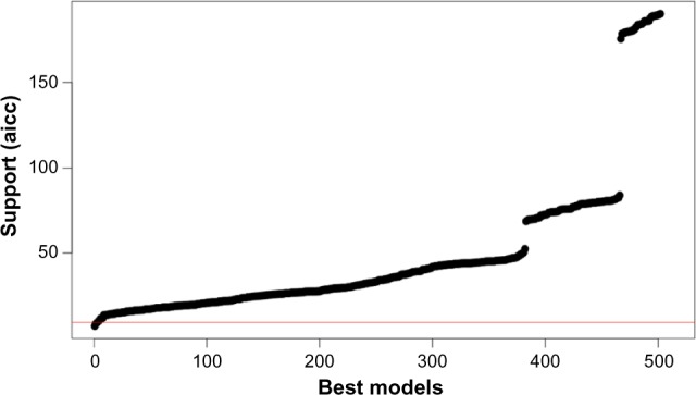
Information criterion profile of all possible model combinations through the wrapper evaluation.
Figure 5.

Model-averaged importance of the statistically significant parameters.
According to Figure 5, the three top-ranked parameters are the 95th percentile of the transit times in the whole region of tumor, the 5th percentile of the permeability surface area product in the “Full Heterogeneous” subregion, and 30th percentile of the plasma volume in the “Full Homogeneous” subregion, which are also the same three explanatory variables of the optimal multivariate linear regression model. Capillary transit times are indicative of hypoxia and provide important information about tumor pathophysiology. Therefore, this biomarker can be potentially related with oxygenation and patient outcome. Permeability surface area product in the “Full Heterogeneous” subregion is also a potentially meaningful biomarker since increased permeability can be attributed to a highly heterogeneous vascular bed, one of the hallmarks of malignant tumors that results in contrast leakage within the tumor tissue. It is also important to mention that ETM provided only one statistically significant parameter, the 70th percentile of ktrans, in the whole tumor area and is related to the wash-in rate of the CA in the tissue which is the most indicative characteristic of a disrupted BBB. As can be noted in Figure 5, highly ranked parameters are also the 30th and 70th percentile of the blood plasma volume in the “Full Homogeneous” subregion. The high accuracy of this parameter in the classification might be due to the expected alteration in the vasculature of a responder, but there is no published data yet to support this. Concerning the rest of the parameters shown in Figure 5, they were found to be less significant in our study.
The statistical analysis was extended in the context of identifying any potential discrimination between subpopulations “Immune Reaction” and “Response” within the “Res ponse” group. To this end, the statistical analysis framework using AICc as the criterion for selecting the parameters with the optimum discriminatory power was applied to a cohort of four samples/patients (two patients in each group). Despite the fact that more than 50 from the 588 parameters achieved accuracy of 100%, their estimated P-values were declared as statistically insignificant (P-value >0.12). Consequently, all parameters failing to meet the criterion of the P-value threshold at the preprocessing phase (<1%) were excluded from the linear model combination process. Also, a Lasso regression model was applied to the same cohort of 588 parameters, using LOO-CV for tuning the model and calculating its nonzero coefficients. All the returned coefficients had a zero value; thus the analysis failed to define a model for predicting accurately the treatment response outcome of the examined cohort. In conclusion, the analysis showed that both models have no predictive power in classifying correctly the subpopulations “response” and “immune reaction” for the specific dataset that was used in the analysis.
Discussion
Biomarkers extracted from DCE-MRI have been used in several studies for the prediction of therapeutic outcome to chemoradiation36,37 and therapies that target vasculature1,6,38–40 in several tumor types,1,41–43 as well as for the grading of gliomas through histogram analysis.44 All these studies indicate that the relative changes of the DCE biomarkers have the potential to predict or assess patient outcome. However, pertinent studies are needed to define the actual meaning of these parameters and to confirm their robustness in describing tumor vascular heterogeneity.
In our work, statistical analysis was performed on the results derived from two PK models, the well-established ETM and the more recent GCTT; the latter has shown initial promising results in the literature.45,46 The statistical analysis was able to differentiate responders from nonresponders, although the cohort of patients was relatively small (N = 11) and all subjects were diagnosed with GBM. The statistical analysis indicates that the GCCT model outperforms ETM. This is in line with results from previous research,23 where authors argue that GCTT biomarkers are expected to be more robust. The previous assumption is reliable, given that the IRF of the model is able to be adapted to the specific tissue (per voxel) based on the heterogeneity of the transit times by adjusting the α−1 parameter. Moreover, results derived from three different types of brain tumors23 (GBM, pleomorphic xanthoastrocytoma, and anaplastic meningioma) have shown remarkable discrepancies in DCE biomarker values when different PK models were used. This inconsistency could be attributed, according to previous work,22 to the fact that TM is accurate only in weakly vascularized tissues while ETM is also accurate in highly perfused tissues, but considering that tumor vasculature is highly heterogeneous, a model such as TM or ETM that assumes a single capillary transit time is expected to diverge from reality in certain cases.
In essence, the GCCT model generalizes well-established models that have been extensively used so far and offers a new variable (α−1) that describes vascular heterogeneity. In this work we proposed an additional preprocessing step by exploiting the α−1 parameter. The tumor region of interest was segmented into four sub-regions based on the aforementioned parameter. Although these bounds were determined empirically, after several experiments we found that the classification outcome was not affected by small perturbations in the proposed boundary values for each subregion. However, when only three subregions were used instead of four, the classification failed to give satisfactory results. Finally, considering the limited number of patients and the restriction to only GBM tumor, the proposed classification based on α−1 boundaries should be verified in a more extensive patient group. A thorough sensitivity analysis should be performed as well in order to define consistent subregion boundaries that could be used prospectively in clinical decision support.
In our study, the GCTT model’s PK parameters performed better than Tofts’, while the segmentation of the tumor ROIs based on vascular heterogeneity further enhanced the discriminatory power of the GCTT model. The results indicate that the GCTT model may be more efficient in characterizing the chaotic vascular structure of tumor and subsequent pathophysiological characteristics such as the delayed extraction of the CA in the EES. Also, in search for the best model according to the optimal multivariate linear regression presented, the GCCT PK parameters outperformed the Tofts ones. ktrans computed from ETM performed well in our study, and in particular the 70% percentile. Figure 6 shows the histogram profiles for ktrans for all the patients. The ROC results showed, however, that the overall best PK parameter is the extraction fraction E (70% percentile) of the GCCT model but only when computed in the “Heterogeneous” subregion (in tables of results referred to as region 3). This is further highlighted in Figure 7, where it can be observed that the histograms of this parameter between responders and nonresponders become morphologically more separable in the “Heterogeneous” subregion than in the whole tumor ROI as annotated in the MRI data. If this result is confirmed in future studies, it has the potential to enhance the robustness of PK imaging biomarkers from DCE-MRI and widen their clinical adoption for aiding the therapy monitoring process. However, being aware of the limited cohort group of this study and the restriction to only GBM tumor, we suggest more extensive studies in a broader range of patients and tumor types in order to establish which model is better for the early prediction of response in cancer patients.
Figure 6.
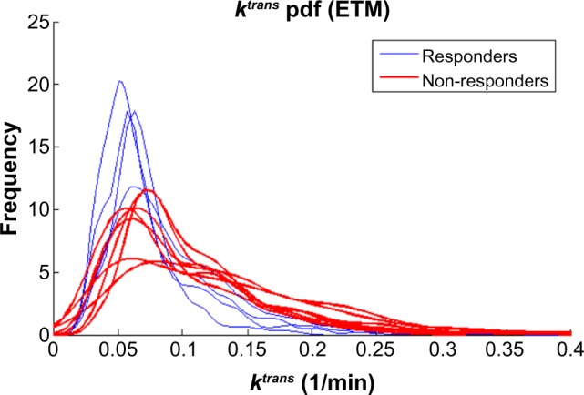
ktrans PK parameter computed in the whole tumor region of interest also offers a good separability while the 70% percentile was the best metric.
Figure 7.
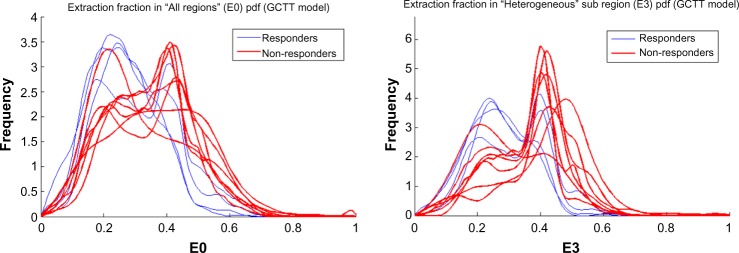
Histograms for the extraction fraction GCCT model parameter E for the whole tumor ROI (left) and the “Heterogeneous” subregion (right). It can be observed that there is a morphological enhancement in terms of separability between responders and nonresponders in the “Heterogeneous” subregion in comparison to the whole tumor ROI as annotated in the MRI data.
Appendix
Abbreviation and symbols are presented in Table A1 while Table A2 summarizes the PK parameters derived from DCE-MRI data.
Table A1.
Abbreviation and symbols.
| ADC | Apparent diffusion coefficient |
| AIF | Arterial input function |
| AIC | Akaike information criterion |
| AICc | Small-sample corrected akaike information criterion |
| ATH | Adiabatic tissue homogeneity |
| AUCs | Areas under the roc-curve |
| BBB | Blood brain barrier |
| CA | Contrast agent |
| DCE-MRI | Dynamic contrast-enhanced magnetic resonance imaging |
| EES | Extracellular extravascular space |
| ETM | Extended tofts model |
| FN | False negative |
| FP | False positive |
| GBM | Glioblastoma multiforme |
| GCTT | Gamma capillary transit time |
| Gd | Gadolinium |
| IRF | Impulse response function |
| MRI | Magnetic resonance imaging |
| MTT | Mean transit time |
| PK | Pharmacokinetic |
| rCBF | Regional cerebral blood flow |
| rCBV | Regional cerebral blood volume |
| ROC | Receiver operator characteristics |
| ROI | Region of interest |
| SNR | Signal to noise ratio |
| SPGR | Spoiled gradient echo |
| TM | Tofts model |
| TN | True negative |
| TP | True positive |
| VOI | Volume of interest |
| 2CX | Two compartment exchange |
Table A2.
PK parameters derived from DCE-MRI data.6
| PARAMETER | DEFINITION | UNIT |
|---|---|---|
| Models parameters | ||
| F | Blood flow (normalized by tissue volume) | mL/mL/min−1 |
| E | Extraction fraction | none |
| ktrans | Volume transfer constant between plasma and EES | min−1 |
| kep | Rate constant between EES and plasma | min−1 |
| τ | Scale parameter of gamma distribution | sec |
| α−1 | Distribution of capillary transit times | none |
| vp | Blood plasma volume per unit volume of tissue | none |
| ve | EES volume per unit volume of tissue | none |
| Additional parameters | ||
| PS | Permeability surface area product per unit mass of tissue | mL/mL/min−1 |
| tc | Capillary transit time | sec |
| Biophysical parameters | ||
| T10 | Pre-contrast longitudinal relaxation time | sec |
| T1(t) | Post-contrast longitudinal relaxation time | sec |
| S0 | Equilibrium magnetization | none |
| Ct(t) | Concentration in tissue | mM |
| Ca(t) | Concentration in artery blood (AIF) | mM |
| IRFv(t) | Vascular impulse response function | none |
| IRFp(t) | Parenchyma impulse response function | none |
| Hct | Hematocrit | none |
| Imaging parameters | ||
| TS | Temporal sampling interval | sec |
| TR | Repetition time | sec |
| S1 | Signal intensity | none |
| α | Flip Angle (FA) | degrees |
| αf | Variable Flip Angle (VFA) | degrees |
| r1 | Relaxation constant of the contrast agent | sec−1·mM−1 |
Footnotes
ACADEMIC EDITOR: J.T. Efird, Editor in Chief
FUNDING: KM, EK, GM, and GK acknowledge the internal funding support of FORTH-ICS for the development of the perfusion MRI methods and software. All authors acknowledge support for the analysis of the clinical data with the above software and methods from the European Union Seventh Framework Programme under grant agreement number 600841, Computational Horizons in Cancer (CHIC; http://www.chic-vph.eu). The authors confirm that the funder had no influence over the study design, content of the article, or selection of this journal.
COMPETING INTERESTS: Authors disclose no potential conflicts of interest.
Paper subject to independent expert blind peer review by minimum of two reviewers. All editorial decisions made by independent academic editor. Upon submission manuscript was subject to anti-plagiarism scanning. Prior to publication all authors have given signed confirmation of agreement to article publication and compliance with all applicable ethical and legal requirements, including the accuracy of author and contributor information, disclosure of competing interests and funding sources, compliance with ethical requirements relating to human and animal study participants, and compliance with any copyright requirements of third parties. This journal is a member of the Committee on Publication Ethics (COPE).
Author Contributions
Conceived and designed the experiments: KM, SVC. Analyzed the data: EK, GK. Statistical analysis: GM. Wrote the first draft of the manuscript: EK, GK, GM. Contributed to the writing of the manuscript: KM. Clinical input and data: SVC. All authors read and approved the final manuscript.
REFERENCES
- 1.O’Connor JP, Jackson A, Parker GJ, Jayson GC. DCE-MRI biomarkers in the clinical evaluation of antiangiogenic and vascular disrupting agents. Br J Cancer. 2007;96:189–95. doi: 10.1038/sj.bjc.6603515. [DOI] [PMC free article] [PubMed] [Google Scholar]
- 2.Wolburg H, Lippoldt A. Tight junctions of the blood-brain barrier: development, composition and regulation. Vascul Pharmacol. 2002;38:323–37. doi: 10.1016/s1537-1891(02)00200-8. [DOI] [PubMed] [Google Scholar]
- 3.Bergamino M, Saitta L, Barletta L, et al. Measurement of blood-brain barrier permeability with t1-weighted dynamic contrast-enhanced MRI in brain tumors: a comparative study with two different algorithms. ISRN Neurosci. 2013;2013:905279. doi: 10.1155/2013/905279. [DOI] [PMC free article] [PubMed] [Google Scholar]
- 4.Cramer SP, Simonsen H, Frederiksen JL, Rostrup E, Larsson HB. Abnormal blood-brain barrier permeability in normal appearing white matter in multiple sclerosis investigated by MRI. Neuroimage Clin. 2014;4:182–9. doi: 10.1016/j.nicl.2013.12.001. [DOI] [PMC free article] [PubMed] [Google Scholar]
- 5.Abo-Ramadan U, Durukan A, Pitkonen M, et al. Post-ischemic leakiness of the blood-brain barrier: a quantitative and systematic assessment by Patlak plots. Exp Neurol. 2009;219(1):328–33. doi: 10.1016/j.expneurol.2009.06.002. [DOI] [PubMed] [Google Scholar]
- 6.O’Connor JP, Jackson A, Parker GJ, Roberts C, Jayson GC. Dynamic contrast-enhanced MRI in clinical trials of antivascular therapies. Nat Rev Clin Oncol. 2012;9(3):167–77. doi: 10.1038/nrclinonc.2012.2. [DOI] [PubMed] [Google Scholar]
- 7.Yankeelov TE, Lepage M, Chakravarthy A, et al. Integration of quantitative DCE-MRI and ADC mapping to monitor treatment response in human breast cancer: initial results. Magn Reson Imaging. 2007;25:1–13. doi: 10.1016/j.mri.2006.09.006. [DOI] [PMC free article] [PubMed] [Google Scholar]
- 8.De Langen AJ, Van Den Boogaart VE, Marcus JT, Lubberink M. Use of H2(15)O-PET and DCE-MRI to measure tumor blood flow. Oncologist. 2008;13(6):631–44. doi: 10.1634/theoncologist.2007-0235. [DOI] [PubMed] [Google Scholar]
- 9.Weinmann H, Laniado M, Mützel W. Pharmacokinetics of Gd-DTPA/dimeglumine after intravenous injection into healthy volunteers. Physiol Chem Phys Med NMR. 1984;16(2):167–72. [PubMed] [Google Scholar]
- 10.Gadian DG, Payne JA, Bryant DJ, Young IR, Carr DH, Bydder GM. Gadolinium-DTPA as a contrast agent in MR imaging – theoretical projections and practical observations. J Comput Assist Tomogr. 1985;9:242–51. doi: 10.1097/00004728-198503000-00003. [DOI] [PubMed] [Google Scholar]
- 11.Ordidge RJ, Gibbs P, Chapman B, Stehling MK, Mansfield P. High-speed multislice T 1 mapping using inversion-recovery echo-planar imaging. Magn Reson Med. 1990;16:238–45. doi: 10.1002/mrm.1910160205. [DOI] [PubMed] [Google Scholar]
- 12.Studler U, White LM, Andreisek G, Luu S, Cheng HL, Sussman MS. Impact of motion on T1 mapping acquired with inversion recovery fast spin echo and rapid spoiled gradient recalled-echo pulse sequences for delayed gadolinium-enhanced MRI of cartilage (dGEMRIC) in volunteers. J Magn Reson Imaging. 2010;32:394–8. doi: 10.1002/jmri.22249. [DOI] [PubMed] [Google Scholar]
- 13.Zhu DC, Penn RD. Full-brain T1 mapping through inversion recovery fast spin echo imaging with time-efficient slice ordering. Magn Reson Med. 2005;54:725–31. doi: 10.1002/mrm.20602. [DOI] [PubMed] [Google Scholar]
- 14.Henderson E, McKinnon G, Lee TY, Rutt BK. A fast 3D look-locker method for volumetric T1 mapping. Magn Reson Imaging. 1999;17(8):1163–71. doi: 10.1016/s0730-725x(99)00025-9. [DOI] [PubMed] [Google Scholar]
- 15.Freeman AJ, Gowland PA, Mansfield P. Optimization of the ultrafast look-locker echo-planar imaging T1 mapping sequence. Magn Reson Imaging. 1998;16(7):765–72. doi: 10.1016/s0730-725x(98)00011-3. [DOI] [PubMed] [Google Scholar]
- 16.Wang HZ, Riederer SJ, Lee JN. Optimizing the precision in T1 relaxation estimation using limited flip angles. Magn Reson Med. 1987;5:399–416. doi: 10.1002/mrm.1910050502. [DOI] [PubMed] [Google Scholar]
- 17.Cheng H-L, Wright G. Rapid high-resolution T1 mapping by variable flip angles: accurate and precise measurements in the presence of radiofrequency field inhomogeneity. Micron. 2006;37:566–76. doi: 10.1002/mrm.20791. [DOI] [PubMed] [Google Scholar]
- 18.Andreisek G, White LM, Yang Y, Robinson E, Cheng H-LM, Sussman MS. Delayed gadolinium-enhanced MR imaging of articular cartilage: three-dimensional T1 mapping with variable flip angles and B1 correction. Radiology. 2009;252(3):865–73. doi: 10.1148/radiol.2531081115. [DOI] [PubMed] [Google Scholar]
- 19.Brix G, Salehi Ravesh M, Zwick S, Griebel J, Delorme S. On impulse response functions computed from dynamic contrast-enhanced image data by algebraic deconvolution and compartmental modeling. Phys Med. 2012;28:119–28. doi: 10.1016/j.ejmp.2011.03.004. [DOI] [PubMed] [Google Scholar]
- 20.Tofts PS, Kermode AG. Measurement of the blood-brain barrier permeability and leakage space using dynamic MR imaging. 1. Fundamental concepts. Magn Reson Med. 1991;17(2):357–67. doi: 10.1002/mrm.1910170208. [DOI] [PubMed] [Google Scholar]
- 21.Tofts PS. Modeling tracer kinetics in dynamic Gd-DTPA MR imaging. J Magn Reson Imaging. 1997;7:91–101. doi: 10.1002/jmri.1880070113. [DOI] [PubMed] [Google Scholar]
- 22.Sourbron SP, Buckley DL. On the scope and interpretation of the Tofts models for DCE-MRI. Magn Reson Med. 2011;66:735–45. doi: 10.1002/mrm.22861. [DOI] [PubMed] [Google Scholar]
- 23.Schabel MC. A unified impulse response model for DCE-MRI. Magn Reson Med. 2012;68:1632–46. doi: 10.1002/mrm.24162. [DOI] [PubMed] [Google Scholar]
- 24.Zhou J, Wilson DA, Ulatowski JA, Traystman RJ, van Zijl PC. Two-compartment exchange model for perfusion quantification using arterial spin tagging. J Cereb Blood Flow Metab. 2001;21:440–55. doi: 10.1097/00004647-200104000-00013. [DOI] [PubMed] [Google Scholar]
- 25.St Lawrence KS, Lee T. An adiabatic approximation to the tissue homogeneity model for water exchange in the brain. J Cereb Blood Flow Metab. 1998;18(12):1365–77. doi: 10.1097/00004647-199812000-00011. [DOI] [PubMed] [Google Scholar]
- 26.Koh TS, Zeman V, Darko J, et al. The inclusion of capillary distribution in the adiabatic tissue homogeneity model of blood flow. Phys Med Biol. 2001;46(5):1519–38. doi: 10.1088/0031-9155/46/5/313. [DOI] [PubMed] [Google Scholar]
- 27.Wen PY, Macdonald DR, Reardon DA, et al. Updated response assessment criteria for high-grade gliomas: response assessment in neuro-oncology working group. J Clin Oncol. 2010;28(11):1963–72. doi: 10.1200/JCO.2009.26.3541. [DOI] [PubMed] [Google Scholar]
- 28.Kruskal W, Allen W. Use of ranks in one-criterion variance analysis. J Am Stat Assoc. 1952;47:583–621. [Google Scholar]
- 29.Cavanaugh JE. Unifying the derivations for the Akaike and corrected Akaike information criteria. Stat Probab Lett. 1997;33:201–8. [Google Scholar]
- 30.Akaike H. A new look at the statistical model identification. IEEE Trans Automat Contr. 1974;19:716–23. [Google Scholar]
- 31.Burnham KP, Anderson DR. Model selection and multimodel inference a practical information-theoretic approach. 2nd ed. New York: Springer; 2002. [Google Scholar]
- 32.Development Core Team . R: A Language and Environment for Statistical Computing. R Foundation for Statistical Computing; Vienna, Austria: 2011. 3-900051-07-0. [Google Scholar]
- 33.Robin X, Turck N, Hainard A. pROC: an open-source package for R and S+ to analyze and compare ROC curves. BMC Bioinformatics. 2011;12(1):77. doi: 10.1186/1471-2105-12-77. [DOI] [PMC free article] [PubMed] [Google Scholar]
- 34.Calcagno V, De Mazancourt C. glmulti: an R package for easy automated model selection with (generalized) linear models. J Stat Softw. 2010;34(12):1–29. [Google Scholar]
- 35.Baclawski K. J Stat Softw. 2009 Apr;30:1–3. [Google Scholar]
- 36.Semple SI, Harry VN, Parkin DE, Gilbert FJ. A combined pharmacokinetic and radiologic assessment of dynamic contrast-enhanced magnetic resonance imaging predicts response to chemoradiation in locally advanced cervical cancer. Int J Radiat Oncol Biol Phys. 2009;75(2):611–7. doi: 10.1016/j.ijrobp.2009.04.069. [DOI] [PubMed] [Google Scholar]
- 37.Andersen EK, Hole KH, Lund KV, et al. Pharmacokinetic parameters derived from dynamic contrast enhanced MRI of cervical cancers predict chemoradio-therapy outcome. Radiother Oncol. 2013;107:117–22. doi: 10.1016/j.radonc.2012.11.007. [DOI] [PubMed] [Google Scholar]
- 38.Mehta S, Hughes NP, Buffa FM, et al. Assessing early therapeutic response to bevacizumab in primary breast cancer using magnetic resonance imaging and gene expression profiles. J Natl Cancer Inst Monogr. 2011;2011(43):71–4. doi: 10.1093/jncimonographs/lgr027. [DOI] [PubMed] [Google Scholar]
- 39.Hahn OM, Yang C, Medved M, et al. Dynamic contrast-enhanced magnetic resonance imaging pharmacodynamic biomarker study of sorafenib in metastatic renal carcinoma. J Clin Oncol. 2008;26(28):4572–8. doi: 10.1200/JCO.2007.15.5655. [DOI] [PMC free article] [PubMed] [Google Scholar]
- 40.Najafi M, Soltanian-Zadeh H, Jafari-Khouzani K, Scarpace L, Mikkelsen T. Prediction of glioblastoma multiform response to bevacizumab treatment using multi-parametric MRI. PLoS One. 2012;7(1):1–11. doi: 10.1371/journal.pone.0029945. [DOI] [PMC free article] [PubMed] [Google Scholar]
- 41.Jackson A, O’Connor JP, Parker GJ, Jayson GC. Imaging tumor vascular heterogeneity and angiogenesis using dynamic contrast-enhanced magnetic resonance imaging. Clin Cancer Res. 2007;13(12):3449–59. doi: 10.1158/1078-0432.CCR-07-0238. [DOI] [PubMed] [Google Scholar]
- 42.Khalifa F, Soliman A, El-Baz A, et al. Models and methods for analyzing DCE-MRI: a review. Med Phys. 2014;41(12):124301. doi: 10.1118/1.4898202. [DOI] [PubMed] [Google Scholar]
- 43.Heye AK, Culling RD, Valdés Hernández Mdel C, Thrippleton MJ, Wardlaw JM. Assessment of blood-brain barrier disruption using dynamic contrast-enhanced MRI. A systematic review. Neuroimage Clin. 2014;6:262–74. doi: 10.1016/j.nicl.2014.09.002. [DOI] [PMC free article] [PubMed] [Google Scholar]
- 44.Jung SC, Yeom JA, Kim JH, et al. Glioma: application of histogram analysis of pharmacokinetic parameters from T1-weighted dynamic contrast-enhanced MR imaging to tumor grading. AJNR Am J Neuroradiol. 2014;35:1103–10. doi: 10.3174/ajnr.A3825. [DOI] [PMC free article] [PubMed] [Google Scholar]
- 45.Jensen RL, Mumert ML, Gillespie DL, Kinney AY, Schabel MC, Salzman KL. Preoperative dynamic contrast-enhanced MRI correlates with molecular markers of hypoxia and vascularity in specific areas of intratumoral microenvironment and is predictive of patient outcome. Neuro Oncol. 2014;16(2):280–91. doi: 10.1093/neuonc/not148. [DOI] [PMC free article] [PubMed] [Google Scholar]
- 46.Jacobs I, Strijkers GJ, Keizer HM, Janssen HM, Nicolay K, Schabel MC. A novel approach to tracer-kinetic modeling for (macromolecular) dynamic contrast-enhanced MRI. Magn Reson Med. 2015 2014 Oct; doi: 10.1002/mrm.25704. [DOI] [PubMed] [Google Scholar]