Bayesian Small Area Estimates of Diabetes Incidence by United States County, 2009

Abstract

In the United States, diabetes is common and costly. Programs to prevent new cases of diabetes are often carried out at the level of the county, a unit of local government. Thus, efficient targeting of such programs requires county-level estimates of diabetes incidence–the fraction of the non-diabetic population who received their diagnosis of diabetes during the past 12 months. Previously, only estimates of prevalence–the overall fraction of population who have the disease–have been available at the county level. Counties with high prevalence might or might not be the same as counties with high incidence, due to spatial variation in mortality and relocation of persons with incident diabetes to another county. Existing methods cannot be used to estimate county-level diabetes incidence, because the fraction of the population who receive a diabetes diagnosis in any year is too small. Here, we extend previously developed methods of Bayesian small-area estimation of prevalence, using diffuse priors, to estimate diabetes incidence for all U.S. counties based on data from a survey designed to yield state-level estimates. We found high incidence in the southeastern United States, the Appalachian region, and in scattered counties throughout the western U.S. Our methods might be applicable in other circumstances in which all cases of a rare condition also must be cases of a more common condition (in this analysis, “newly diagnosed cases of diabetes” and “cases of diabetes”). If appropriate data are available, our methods can be used to estimate proportion of the population with the rare condition at greater geographic specificity than the data source was designed to provide.

1. Introduction

In the United States, diabetes has an enormous social cost (American Diabetes Association, 2008). Persons with diabetes are at increased risk of devastating complications that include blindness (Kertes and Johnson, 2007), hearing loss (Kakarlapudi et al., 2003), and kidney failure (Centers for Disease Control, 2011), and a person with diabetes is at about twice the risk of death as a person of similar age without diabetes (Centers for Disease Control, 2011). Having diabetes approximately doubles one’s medical costs (Centers for Disease Control, 2011).

Diabetes is common, and becoming more so. In 2010, the national incidence (fraction of the population diagnosed in the preceding twelve months) was 8.6 per 1000 person years and the national prevalence (fraction of population who have the condition) of diagnosed diabetes was 6.0% (Centers for Disease Control and Prevention, 2012a). By 2050, the national diabetes incidence is projected to be 15 per 1000 and the national prevalence is projected to be at least 14.8% (Boyle et al., 2010). A child born in 2000 in the United States has a more than 1 in 3 risk of developing diabetes sometime in his or her life (Narayan et al., 2003).

Programs to prevent new cases of diabetes and to prevent complications and diabetes mortality are generally conducted locally, often at the level of the county (a unit of local government in the United States) or county equivalent (hereafter “county”). State-level estimates of the prevalence of diagnosed diabetes have long existed, based on data from the Behavioral Risk Factor Surveillance System (BRFSS), an ongoing, state-based, random-digit-dialed telephone survey of non- institutionalized adults aged > 18 years in all 50 states, the District of Columbia, and some territories (Centers for Disease Control and Prevention, 2012b). County-level prevalence estimates, pinpointing the counties with the greatest need for programs to prevent complications and death among persons with diabetes, have recently been developed, using model-based small area estimation techniques (Cadwell et al., 2010, Congdon and Lloyd, 2010, Srebotnjak, Mokdad and Murray, 2010).

Diabetes incidence and prevalence are obviously related; a person who develops diabetes, with rare exceptions, has the condition for life. However, incidence might or might not be high in areas of high prevalence, with differences stemming from spatial variability in mortality among persons with diabetes (a county with high incidence could have low prevalence, if mortality among persons with diabetes was large) and in mobility; for example, if incident cases in county A relocate to county B, they influence the incidence rate in A but not B, and the prevalence rate in B but not A.

To effectively target programs to prevent diabetes, we must identify areas of high incidence. However, historically, only state-level estimates of diabetes incidence have been available, and only for states that opted to conduct more in-depth interviews of persons with diabetes to determine when they were diagnosed.

Here, expanding on the work of Cadwell et al. (2010), in which BRFSS data were used to estimate county-level prevalence, we provide the first estimates of diabetes incidence for all 3,143 U.S. counties. Our underlying method is based on noticing that all incident cases of diabetes must also be prevalent cases. We first estimate county-level prevalence. We then estimate the county-level proportion of prevalent cases that are incident cases. Multiplying these together yields an estimate of incidence.

2. Methods

2.1 Data Sources

We use BRFSS data to model diabetes incidence. The BRFSS is a collection of cross-sectional random-digit-dialing telephone surveys, conducted in all U.S. states and the District of Columbia. Every year, states conduct monthly telephone surveillance using a standardized questionnaire to determine the distribution of risk behaviors and health practices among noninstitutionalized adults. We use U.S. Census data to post-stratify the modeled estimates to be representative of U.S. counties in 2009.

County of residence for BRFSS respondents, while not included in the all versions of the data, was obtained for this study. For respondents with missing county of residence, we used the county most likely associated with the respondent’s telephone number. To make inferences from the sample to the population, post-stratification weights were attached to estimates. This use of post-stratification weights guarantees that our estimates are consistent with U.S. Census estimates of county population size.

For respondents indicating that they had diagnosed diabetes, an optional diabetes module was administered in some states in some years. On average, 41 states administered the diabetes module during 2008 through 2010, the years of data we used (combining three years of data follows the precedent set by Cadwell et al., and this approach was chosen because using fewer years resulted in some unstable estimates, due to smaller sample size). This results in some states having one year of data, some two years, and some three. One state had no diabetes module data.

The U.S. Census Bureau publishes population estimates by demographic characteristics (unit-level auxiliary information) for all counties (U.S. Census, 2012); the Census provides no information on diabetes status. We used the 2009 U.S. Census county projections to obtain estimates for the number of persons in each of the classes into which we group BRFSS data.

2.2 Diabetes Information Gathered

All BRFSS respondents were asked, “Have you ever been told by a doctor that you have diabetes?” Those who responded “no” were considered to not have diagnosed diabetes. Males who responded “yes” were considered to have diabetes. Females who responded “yes” were asked if they were told only during pregnancy. Those who indicated this had happened were considered have had gestational diabetes, which resolves at delivery, and were not considered to have diabetes. Females who had been told at any other time were considered to have diabetes. Respondents who did not know or refused to answer the question were considered to have missing diabetes status.

Those who indicated that they had diagnosed diabetes and resided in states that administered the optional diabetes module were asked, “How old were you when you were told you have diabetes?” Age at the time of the survey and age at diagnosis, both self-reported, are measured in years and used to estimate the number of incident cases (2012a). If the difference between a respondent’s age and age at diagnosis is two or more years, the person is not considered an incident case. If the difference is zero years, the person is considered an incident case. If the difference is one year, the person is weighted as half an incident case; this method has been used previously to estimate diabetes incidence (Centers for Disease Control and Prevention, 2012a).

2.3 Incidence Modeling with Missing Data

The general framework for our model-based approach includes multilevel modeling followed by post-stratification (Gelman and Hill 2007, Chapter 14). Because of missing data, we use an approach analogous to “factoring the likelihood” (Little and Rubin 2002, Chapter 7). We specify a full Bayesian probability model that allows the posterior distribution to be factored into two parts that are estimated separately. Unlike the perhaps more familiar complete case analysis, this methods uses all the information on diabetes in the responses for which diabetes incidence status is missing.

Let Z₁ = 1 if an individual was diagnosed with diabetes within the past year; Z₁ = 0 otherwise. Let Z₂ = 1 if an individual was diagnosed with diabetes; Z₂ = 0 otherwise. Since the distribution of prevalence given incidence, p(Z₂|Z₁), equals one, the distribution of incidence, p(Z₁), can be written as p(Z₁, Z₂) = p(Z₁|Z₂)p(Z₂). We develop separate models for incidence conditioned on the person being a prevalent case, p(Z₁|Z₂), and for prevalence, p(Z₂). The estimates from the two models are combined to obtain an estimate of incidence, p(Z₁). Assuming the parameters in the conditional incidence model and the prevalence model are distinct allows the distribution of incidence to be split into these two parts. See Appendix 1 for details.

For each of the 3,143 U.S. counties, sampled persons were cross-classified by age group (20–44, 45–64, 65+ years), sex (male, female) and race/ethnicity (non-Hispanic white, other); sample sizes did not support a finer division of race/ethnicity. This results in 12 classes per county. The number of people sampled in each class who have diabetes can be determined. Specifically, let n_ij = the number of sampled people in county i, class j = 1, ⋯, 12, and y_ij= the number of sampled people with diagnosed diabetes in county i, class j. In some years, in some counties, n_ij = 0. For each of these, the corresponding y_ij = 0. Let y_ij* = the number of sampled people with diagnosed diabetes in county i, class j = 1, ⋯, 12, whose incident status is known and r_ij = the number of sampled people with incident diabetes in county i, class j.

2.4 Prevalence Model

We fit a Bayesian multilevel model to the three years of BRFSS data, using methods similar to Cadwell et al., 2010, but differing in several ways (e.g., we used a Binomial distribution with a logit link instead of the Poisson distribution and logarithmic link that Cadwell et al. used). Our model and Cadwell et al.’s model yield similar, but not identical, estimates. Our changes reduce the number of approximations (e.g., Cadwell et al. used the Poisson distribution to approximate the Binomial, while we used the Binomial).

Our model relates observed quantities to the twelve classes. In particular,

$$y_{\mathit{ij}}\sim \text{Binomial}(p_{\mathit{ij}},n_{\mathit{ij}});i=1,\cdots ,3143,j=1,\cdots ,12,$$ (2.1)

where p_ij = the prevalence of diagnosed diabetes in county i, class j. Let s(i) denote the state s that contains county i. The regression model includes:

1. logit link function log(p_ij/(1 − p_ij)).

2. fixed effect intercept for each class (age by sex by race/ethnicity group) ${\alpha }_{p_j};j=1,\cdots ,12$.

3. random effects by county and class ${\mu }_{p_{\mathit{ij}}};i=1,\cdots ,3143,j=1,\cdots ,12$.

4. random effects by state and class ${\nu }_{p_{s(i)j}};s(i)=1,\cdots ,51,j=1,\cdots ,12$.

5. spatial effects by state and class ${\omega }_{p_{s(i)j}};s(i)=1,\cdots ,51,j=1,\cdots ,12$.

Parameters under (c) and (d) are modeled via 12-dimensional multivariate normal priors (Gelfand, Hills, Racine-Poon and Smith, 1990). Parameters under (e) are modeled via 12-dimensional multivariate normal conditional autoregressive priors (Besag, York and Mollie, 1991). The subscript “p” is used to indicate prevalence. Thus the regression model is

$$\mathrm{logit}(p_{\mathit{ij}})={\alpha }_{p_j}+{\mu }_{p_{\mathit{ij}}}+{\nu }_{p_{s(i)j}}+{\omega }_{p_{s(i)j}}.$$ (2.2)

To assess this extended model, we consider a basic model (Rao, 2003) as a benchmark. The basic model includes fixed effects for class and a spatially unstructured random effect for county. The basic regression model is

$$\mathrm{logit}(p_{\mathit{ij}})={\alpha }_{p_j}+{\epsilon }_i.$$ (2.3)

All prior distributions appear in Appendix 2.

2.5 Conditional Incidence Model

The conditional incidence model is similar to the prevalence model:

$$r_{\mathit{ij}}\sim \text{Binomial}(q_{\mathit{ij}},y_{\mathit{ij}}^{\ast });i=1,\cdots ,3143,j=1,\cdots ,12,$$ (2.4)

where q_ij = the probability of incident diabetes among people with diabetes in county i, class j. Let s(i) denote the state s that contains county i. The regression model includes:

1. logit link function log(q_ij/(1 − q_ij)).

2. fixed effect intercept for each class (age by sex by race/ethnicity group) ${\alpha }_{c_j};j=1,\cdots ,12$.

3. random effects by county and class ${\mu }_{c_{\mathit{ij}}};i=1,\cdots ,3143,j=1,\cdots ,12$.

4. random effects by state and class ${\nu }_{c_{s(i)j}};s(i)=1,\cdots ,51,j=1,\cdots ,12$.

5. spatial effects by state and class ${\omega }_{c_{s(i)j}};s(i)=1,\cdots ,51,j=1,\cdots ,12$.

The subscript “c” is used to indicate “conditional incidence”, and to clearly distinguish these parameters from the ones in the prevalence model. As before, parameters under (c) and (d) are modeled via 12-dimensional multivariate normal priors. Parameters under (e) are modeled via 12-dimensional multivariate normal conditional autoregressive priors. Thus the regression model is:

$$\mathrm{logit}(q_{\mathit{ij}})={\alpha }_{c_j}+{\mu }_{c_{\mathit{ij}}}+{\nu }_{c_{s(i)j}}+{\omega }_{c_{s(i)j}}.$$ (2.5)

We again consider a basic model as a benchmark. The basic model includes fixed effects for class and a random effect for county. The basic regression model is

$$\mathrm{logit}(q_{\mathit{ij}})={\alpha }_{c_j}+{\epsilon }_i.$$ (2.6)

All prior distributions appear in Appendix 2.

2.6 Estimates of Diabetes Incidence

Let N_ij = the estimated number of people in county i, class j = 1, ⋯, 12, in 2009 from U.S. Census Bureau. Let ${\tilde{p}}_{\mathit{ij}}$ and ${\tilde{q}}_{\mathit{ij}}$ be draws from the posterior distributions of p_ij and q_ij, respectively. Our estimate of the number of incident diabetes cases in county i is the mean of the posterior predictive distribution of:

$${\displaystyle \sum _j{\tilde{p}}_{\mathit{ij}}}{\tilde{q}}_{\mathit{ij}}{N}_{\mathit{ij}}.$$ (2.7)

The estimate of the annual incidence rate in county i is the mean of the posterior predictive distribution of:

$$\frac{{\displaystyle {\sum }_j{\tilde{p}}_{\mathit{ij}}{\tilde{q}}_{\mathit{ij}}{N}_{\mathit{ij}}}}{[{\displaystyle {\sum }_j}{N}_{\mathit{ij}}-{\displaystyle {\sum }_j{\tilde{p}}_{\mathit{ij}}(1-{\tilde{q}}_{\mathit{ij}})N_{\mathit{ij}}}]}.$$ (2.8)

Note that the denominator in the above expression is an estimate of the number of nondiabetic persons in county i at the start of 2009. The estimate of the age specific number of incident diabetes cases in county i, age group k is the mean of the posterior predictive distribution of:

$${\displaystyle \sum _{j\in A_k}{\tilde{p}}_{\mathit{ij}}{\tilde{q}}_{\mathit{ij}}{N}_{\mathit{ij}}},$$ (2.9)

where A_k is the set of classes for age group k. The estimate of the age specific annual incidence rate in county i, age group k is the mean of the posterior predictive distribution of:

$${\widehat{p}}_{\mathit{ik}}=\frac{{{\displaystyle \sum }}_{{j\in A}_k}{\tilde{p}}_{\mathit{ij}}{\tilde{q}}_{\mathit{ij}}{N}_{\mathit{ij}}}{[{{\displaystyle \sum }}_{{j\in A}_k}{N}_{\mathit{ij}}-{{\displaystyle \sum }}_{{j\in A}_k}{\tilde{p}}_{\mathit{ij}}(1-{\tilde{q}}_{\mathit{ij}})N_{\mathit{ij}}]}.$$ (2.10)

Then the age-adjusted annual incidence rate for county i is the mean of the posterior predictive distribution of:

$${\widehat{p}}_i={\displaystyle \sum _k{w}_k{\widehat{p}}_{\mathit{ik}}},$$ (2.11)

where w_k is the proportion of the U.S. population in age group k as measured by the 2000 U.S. Census.

All posterior distributions were simulated in WinBUGS (Lunn et al., 2000). The 2.5th and 97.5th percentiles of the posterior distributions provide the 95% posterior intervals for county incidence of diagnosed diabetes. We treat the posterior intervals as confidence intervals. We run two chains, each with a burn-in of 1000 iterations followed by an additional 12,000 iterations. We check convergence by visual inspection of history and autocorrelation plots and using the Gelman-Rubin statistic, as modified by Brooks and Gelman (1998).

2.7 Model Comparisons

We evaluate the frequentist properties of the Bayesian estimates that we calculate using the model selection criterion developed in Gelfand and Ghosh (1998). This criterion depends on a statistic D, which combines goodness-of-fit and variability. Calculating D requires replicating the entire data set for each posterior draw of the model parameters. Using these replicates, we compute the posterior predictive mean and variance for each observation. We calculate G, a goodness of fit measure, as the sum over all observations of the squared difference between the data and its posterior predictive mean. We calculate P, a measure of expected mean square measure, as the sum over all observations of the posterior predictive variances. The statistic D is defined as G+P. Models with smaller D values, meaning that modeled values are more similar to observations, are preferred.

2.8 Model Checking

We implemented posterior predictive checks to examine the consistency of the model with the data (Gelman et al., 2004, Chapter 6.3). In posterior predictive checking, the entire data set is replicated for each posterior draw of the parameters. A discrepancy or test measure that reflects relevant aspects of the model is calculated for each replicate. We used the deviance (McCullagh and Nelder, 1989, Chapter 2.3) as the discrepancy measure. A Bayesian p-value associated with the test measure is calculated; Bayesian p-values differ from the more familiar frequentist p-values in that a value between 0.1 and 0.9 indicates reasonable model fit.

We check our model by comparing it to direct estimates. The BRFSS provides direct, design-based, complete-case estimates of diabetes incidence for 48 states and DC for 2009 (Centers for Disease Control and Prevention, 2012a). These estimates are based on the combined 2008, 2009, 2010 BRFSS data. We aggregate our modeled county estimates to the state level and plot them against the direct estimates, allowing a comparison of modeled and direct estimates.

In an additional model check, we set up a simulation study to evaluate the two-part, prevalence and conditional incidence, modeling approach. Fifteen years of BRFSS data (1996–2010) were combined to create the test population. This test population includes 3,183,766 people, 285,851 with diabetes and 29,048 with incident diabetes. This population is too small to evaluate our model at the county level so we use the fifty states and DC as our “small areas”. The evaluation proceeds as:

1. Sample 20,000 individuals from our population. This approximates the average number of observation per county in three years of BRFSS times 51.

2. Fit the prevalence and conditional incidence models to obtain incidence estimates by the 51 small areas. These models exclude the μ_ij terms.

3. Calculate direct design-based incidence estimates for the 51 small areas.

4. Repeat steps 1, 2 and 3 a total of fifty times.

5. Compare the modeled estimates to the true values from the test population.

6. Compare the direct design-based estimates to the true values from the test population.

Comparisons statistics in step 5 include the difference between the modeled and true values and the root mean squared error divided by the true incidence. Values of the root mean squared error divided by true value less than 0.25 are considered evidence of useful estimates. We generate box plots to visually present the dispersion in the difference between the modeled and true values. In step 6, we calculate the root mean squared error of the design-based estimates divided by the true incidence.

3. Results

3.1 Description of Data

Table 1 provides details (BRFSS data unweighted in this table, since we describe the sample and, at this stage, do not yet make inference to the population) on the number counties and the number of adults 20 years of age or older enumerated in the 2009 Census and surveyed in the 2008–2010 BRFSS. The number of respondents who self-reported diabetes and whose incident status is known also appears. Twelve percent of the BRFSS sample participants reported diagnosed diabetes. Of those, 73% have known incidence status.

Table 1.

Descriptive statistics of the Census and BRFSS data

		BRFSS 2008–2010
	Census 2009	Diabetes Prevalence	Conditional Incidence
Counties	3143	3140	2981
Responses	–	152,391	9676
median (min, max) per county	–	18 (0, 13000)	1 (0, 88)
Observations	223,585,859	1,255,029	110,765
median (min, max) per county	18885 (36, 7057285)	142 (2, 11967)*	14 (1, 1127)*

^*Among counties with greater than zero observations.

3.2 Estimates

There was relatively little variation in county-level conditional incidence (proportion of prevalent cases which are also incident cases); estimated county-level conditional incidence ranged from 0.07 to 0.12, with a median value of 0.10. We looked for spatial patterns in conditional incidence, such as geographic clustering or a tendency to correlate with some demographic, but found no evidence of such patterns (data not shown).

Estimates for incidence for all counties appear in Figure 1. Incidence estimates of diabetes were 0.38%–2.1% (mean 1.1%). The average coefficient of variation was 18% (range, 8%–26%). We also calculate age-adjusted estimates (standardized to the 2000 U.S. population). These differed little from non-age-adjusted ones, and are not reported.

Figure 1.

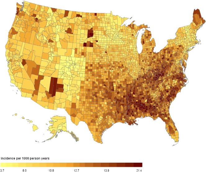
Map of 2009 diabetes incidence for 3143 U.S. counties

3.3 Model Comparisons

Table 2 displays G, P, and D, the model selection criteria. For both prevalence and conditional incidence, the basic model provides a much poorer fit than its competitors. For both prevalence and conditional incidence, the extended model without the spatial effects provides a slightly better fit than the model including the spatial effects. Spatial effects require substantially longer simulation runs for little or no gain. Therefore, we did not include spatial effects in our final estimates.

Table 2.

Model selection criterion

Outcome	Model	Goodness of Fit G	Predictive Error P	D*
Prevalence	Basic	153,335	143,990	297,225
	Extended	65,368	175,465	240,833
	Extended, without spatial	66,310	174,444	240,755
Conditional Incidence	Basic	7084	8765	15,849
	Extended	5594	9783	15,377
	Extended, without spatial	5635	9727	15,362

^*Smaller is better.

The lack of spatial effects in the final model could be viewed as counter-intuitive, since the prevalence of diabetes in the United States (Barker et al., 2011) exhibits strong spatial correlation. However, age, race/ethnicity, and state of residence, factors explicitly considered in our model, are also spatially correlated. These factors also serve as surrogates for factors that directly contribute to the incidence of type 2 diabetes (90–95% of diabetes in the United States [Centers for Disease Control, 2011]), such as obesity, physical inactivity, and lower income/educational achievement. Thus, it is likely that the spatial autocorrelation that remained, after accounting for age, race/ethnicity, and state of residence, was small.

3.4 Model Checking

All models considered had Bayesian p-values between 0.1 and 0.9 (minimum 0.36, maximum 0.81), indicating reasonably good model fit. Figure 2 is a scatterplot of incidence rate per 1000 person-years for direct, design-based estimates (available for 48 states and DC) versus modeled (aggregated up to the state level) estimates. There is good agreement between the estimates with the modeled estimates being slightly higher, on average, than the direct estimates.

Figure 2.

Scatterplot of design-based state incidence versus model-based county incidence aggregated to the state level for 48 states and the District of Columbia

The simulation study showed the modeled estimates to be quite good. Figure 3 displays the root mean squared error over the true value. For all but six of the estimates, the value is less than 0.25. All but four are less than 0.30, and, for most, the ratio is close to 0.15.

Figure 3.

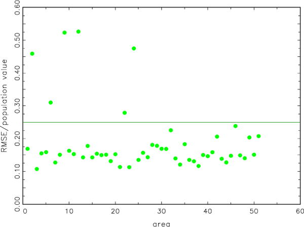
Scatterplot of root mean squared error of model-based incidence estimates over population value versus area. Results are averaged over 50 random samples from the test population

Figure 4 displays boxplots of differences (population minus modeled estimate). Only four states, out of 51 (counting the District of Colombia), have differences that are statistically significantly different from zero at the 0.05 level. The direct, design-based estimates from the simulation study are not usable because of large relative error. For the design-based estimates, the root mean squared errors divided by true values were over 0.30 for all 51 areas, and the median value was 0.54.

Figure 4.

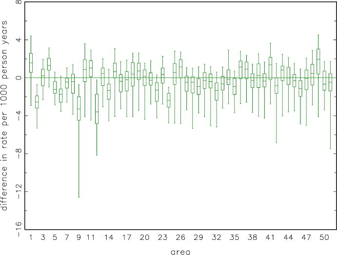
Box plots of difference in incidence, population minus model-based, by area. Each plot box represents 50 random samples from the test population

4. Discussion

We found a concentration of high-incidence counties in the U.S. southeast and in Appalachia, with a scattering of high-incidence counties in the U.S. west, primarily in counties with large American Indian populations. The map, Figure 1, also shows a concentration of low-incidence counties in the state of Colorado. The pattern of county-level diabetes incidence in the U.S. is roughly similar to the pattern of county-level prevalence, in the sense that high-prevalence counties tend to be high-incidence counties as well. Both high-incidence and prevalence, and low-incidence and prevalence counties correlate well with the county-level prevalence of obesity (CDC, 2012), a strong risk factor for type 2 diabetes. The prevalence of obesity is high in the southeast and in Appalachia, and low in Colorado (CDC, 2012). The scattered counties in the west with high diabetes incidence have high prevalence of poverty, another risk factor for type 2 diabetes, and have relatively large populations of American Indians, who are at greater risk of type 2 diabetes than non-Hispanic whites, the majority of the U.S. population.

The strong association of prevalence and incidence estimates suggests that mortality among those with diagnosed diabetes and the rate of relocation to another county after developing diabetes, both of which could cause incidence and prevalence to look very different, are likely be relatively constant across the U.S. This was not known prior to this analysis.

Modeled estimates tended to be slightly larger than direct estimates, as depicted in Figure 2. This is probably due to direct estimates not accounting for those whose incidence status is unknown. Thus, the two estimates have somewhat different denominators, and therefore might be expected to differ.

Among the values of root mean squared error over the true value, Figure 3, there were four possible outliers: Alaska, District of Colombia, Hawaii, and Minnesota. Alaska, District of Colombia, and Hawaii are geographic/demographic outliers in the U.S. We have no explanation for Minnesota’s being on this list.

Our study is subject to several limitations. First, instead of “incidence of diabetes”, we are actually estimating “incidence of diagnosed diabetes”. An estimated 27% of all U.S. diabetes cases are undiagnosed (Centers for Disease Control, 2011). People can have type 2 diabetes, which comprises 90–95% all diabetes (Centers for Disease Control, 2011), for years and be unaware of their condition. No national data set allows us to distinguish “incidence of diabetes” from “incidence of diagnosed diabetes”. Second, our study is subject to the limitations of the BRFSS, such as not adequately representing households that have no land-line telephone (Centers for Disease Control, 2012b). Another limitation of BRFSS is recall bias: people might have simply misremembered the date at which their diabetes was diagnosed (although, for this study, respondents need only categorize diagnosis as: within the current calendar year; in the preceding calendar year; or before the preceding calendar year). In any survey, social desirability bias can exist, although self-report of diagnosed diabetes is usually correct (Okura et al.). Some of the participants in the study whose county of residence was imputed from telephone number might have been incorrectly categorized. This would tend to bias county estimates toward the overall mean. Also, BRFSS does not allow us to distinguish type 2 diabetes from the much less common type 1 diabetes. In our analysis, uncertainty in U. S. Census projections was ignored. This uncertainty is probably small, but not zero; however, the U.S. Census provides what is, by far, the best available estimates of N_ij. Finally, diabetes incidence rates are likely to vary over time. Our methods require at least three years of BRFSS data to produce stable estimates. Thus, we are estimating a running average over time of incidence rates instead of the incident rate for a single year.

Incidence estimates stratified by demographics, such as age or race/ethnicity would have been desirable, since they would have provided insights into the causes of variability among counties in diabetes incidence. However, due to sample size limitations, such estimates have coefficients of variation that we consider unacceptably large. Therefore, we do not report such estimates.

While identifying counties of high and low diabetes incidence is of utility in directing public health interventions in the U.S., our methods have a broader applicability. Neither the methods developed in Cadwell et al. (2010) nor the modified version introduced here can be used to estimate rates of sufficiently rare events, such as diabetes incidence in a single state. However, if the outcome of interest is rare, but all cases of that outcome must also be cases of a more common outcome, our methods might be useful. The fraction of the population with the more common outcome can be estimated. Then the proportion of persons with the rare outcome who also have the more common outcome can be estimated. These estimates can be combined to estimate the faction of the population with the rare outcome. This opens up the possibility of data from BRFSS, or similar surveys in other countries, being used to provide small-area estimates of events that are too rare to be estimated in a one-stage model.

Appendix 1. Factoring the Full Probability Model

Let Z₁ = 1 if an individual was diagnosed with diabetes within the past year; Z₁ = 0 otherwise. Let Z₂ = 1 if an individual was diagnosed with diabetes; Z₂ = 0 otherwise. Let θ = (θ₁, θ₂) be the parameters associated with conditional incidence and prevalence, respectively. Assuming θ₁ is distinct from θ₂ and their prior distributions are independent then

$$\begin{array}{l}(\theta |Z_1,Z_2)=\frac{p(Z_1,Z_2|\theta )p(\theta )}{{\displaystyle \int p(Z_1,Z_2|\theta )p(\theta )d\theta }}\\ =\frac{p(Z_1|Z_2,\theta )p(Z_2|\theta )p(\theta )}{{\displaystyle \int p(Z_1|Z_2,\theta )p(Z_2|\theta )p(\theta )d\theta }}\\ =\frac{p(Z_1|Z_2,{\theta }_1)p({\theta }_1)p(Z_2|{\theta }_2)p({\theta }_2)}{{\displaystyle \int {\displaystyle \int p(Z_1|Z_2,{\theta }_1)p({\theta }_1)p(Z_2|{\theta }_2)p({\theta }_2)d{\theta }_{1}d{\theta }_2}}}\\ =\frac{p(Z_1|Z_2,{\theta }_1)p({\theta }_1)}{{\displaystyle \int p(Z_1|Z_2,{\theta }_1)p({\theta }_1)d{\theta }_1}}\times \frac{p(Z_2,{\theta }_2)p({\theta }_2)}{{\displaystyle \int p(Z_2|Z_2,{\theta }_2)p({\theta }_2)d{\theta }_2}}.\end{array}$$ (A.1)

Therefore the posterior distribution factors into two independent posterior distributions. Each part of the posterior can then be evaluated separately.

Appendix 2. Prior Assumptions

The intercepts by class are assigned improper flat priors, α ≺ 1.

The spatially correlated effects by county and class, ω, are assigned a multivariate normal (MVN) conditional autoregressive prior (Besag, York and Mollie, 1991). Let ω_i = (ω_i1, ω_i2, ⋯, ω_i12)′. Then

$${\omega }_i|{\omega }_{(-i)}\sim \mathcal{M}\mathcal{V}\mathcal{N}({\overline{\omega }}_i,{\sum }_{\omega }),$$ (A.2)

where ω_(−i) equals the matrix ω′ with the i^th column removed, ${\overline{\omega }}_i={\displaystyle {\sum }_{{j\in \delta }_i}{\omega }_j/n_i}$ and δ_i and n_i denote the set of labels of the neighbors of county i and the number of neighbors, respectively, where counties are consider to be “neighbors” if they have a common border. The inverse of Σ_ω is assigned a Wishart prior with scale matrix S_ω and 12 degrees of freedom. The matrix S_ω has ones along the main diagonal and 0.001 for all other elements (Rao, 2003).

The spatially unstructured effects by county and class, μ, are assigned a multivariate (of dimension 14) normal prior with mean zero and variance matrix Σ_μ. The inverse of Σ_μ is assigned a Wishart prior with scale matrix S_μ and 14 degrees of freedom. The matrix S_μ has ones along the main diagonal and 0.001 for all other elements (Rao, 2003). The spatially unstructured effects by state and class, ν, are assigned the same types of priors as μ.

The error terms, ε, in the basic models are assigned a proper half-Cauchy (Gelman and Hill, 2007, Chapter 19) prior distribution with median equal to one. This is a diffuse prior. For this model, its use greatly speeds convergence.

References

- American Diabetes Association. Economic costs of diabetes in the U.S. in 2007. Diabetes Care. 2008;31:1–20. doi: 10.2337/dc08-9017. [DOI] [PubMed] [Google Scholar]
- Barker LE, Kirtland KA, Gregg EW, Geiss LS, Thompson TJ. Geographic distribution of diagnosed diabetes in the United States: a diabetes belt. American Journal of Preventive Medicine. 2011;40:434–439. doi: 10.1016/j.amepre.2010.12.019. [DOI] [PubMed] [Google Scholar]
- Besag J, York J, Mollié A. Bayesian image restoration, with two applications in spatial statistics (with discussion) Annals of the Institute of Statistical Mathematics. 1991;43:1–59. [Google Scholar]
- Brooks SP, Gelman A. Alternative methods for monitoring convergence of iterative simulations. Journal of Computational and Graphical Statistics. 1998;7:434–455. [Google Scholar]
- Boyle JP, Thompson TJ, Gregg EW, Barker LE, Williamson DF. Projection of the year 2050 burden of diabetes in the US adult population: dynamic modeling of incidence, mortality, and prediabetes prevalence. Population Health Metrics. 2010;8:29. doi: 10.1186/1478-7954-8-29. [DOI] [PMC free article] [PubMed] [Google Scholar]
- Cadwell BL, Thompson TJ, Boyle JP, Barker LE. Bayesian small area estimates of diabetes prevalence by U.S. county, 2005. Journal of Data Science. 2010;8:173–188. [PMC free article] [PubMed] [Google Scholar]
- Centers for Disease Control and Prevention. National diabetes fact sheet, 2011. U.S. Department of Health and Human Services, Centers for Disease Control and Prevention. Atlanta, Georgia. Retrieved February. 2011;7:2012. Web site: http://www.cdc.gov/diabetes/pubs/pdf/ndfs_2011.pdf. [Google Scholar]
- Centers for Disease Control and Prevention. National diabetes surveillance system. U.S. Department of Health and Human Services, Centers for Disease Control and Prevention. Atlanta, Georgia. Retrieved February. 2012a;6:2012. Web site: http://www.cdc.gov/diabetes/statistics/ [Google Scholar]
- Centers for Disease Control and Prevention. Behavioral risk factor surveillance system survey data. U.S. Department of Health and Human Services, Centers for Disease Control and Prevention. Atlanta, Georgia. Retrieved February. 2012b;6:2012. Web site: http://www.cdc.gov/brfss/ [Google Scholar]
- Centers for Disease Control and Prevention. Diabetes data and trends. U.S. Department of Health and Human Services, Centers for Disease Control and prevention. Atlanta, Georgia. Retrieved February. 2012c;8:2012. Web site: http://apps.nccd.cdc.gov/DDTSTRS/default.aspx. [Google Scholar]
- Congdon P, Lloyd P. Estimating small area diabetes prevalence in the US using the behavioral risk factor surveillance system. Journal of Data Science. 2010;8:235–252. [Google Scholar]
- Gelfand AE, Ghosh SK. Model choice: a minimum posterior predictive loss approach. Biometrika. 1998;85:1–11. [Google Scholar]
- Gelfand AE, Hills SE, Racine-Poon A, Smith AFM. Illustration of Bayesian inference in normal data models using Gibbs sampling. Journal of the American Statistical Association. 1990;85:972–985. [Google Scholar]
- Gelman A, Carlin JB, Stern HS, Rubin DB. Bayesian Data Analysis. 2nd. Chapman & Hall; New York: 2004. [Google Scholar]
- Gelman A, Hill J. Data Analysis Using Regression and Multilevel/Hierarchical Models. Cambridge University Press; United Kingdom: 2007. [Google Scholar]
- Kakarlapudi V, Sawyer R, Staecker H. The effect of diabetes on sensorineural hearing loss. Otology & Neurotology. 2003;24:382–386. doi: 10.1097/00129492-200305000-00006. [DOI] [PubMed] [Google Scholar]
- Kertes PJ, Johnson TM. Evidence Based Eye Care. Lippincott Williams & Wilkins; Philadelphia, Pennsylvania: 2007. [Google Scholar]
- Little RJA, Rubin DB. Statistical Analysis with Missing Data. 2nd. Wiley; New York: 2002. [Google Scholar]
- Lunn DJ, Thomas A, Best N, Spiegelhalter D. WinBUGS-a Bayesian modeling framework: concepts, structure, and extensibility. Statistics and Computing. 2000;10:325–337. [Google Scholar]
- McCullagh P, Nelder JA. Generalized Linear Models. 2nd. Chapman & Hall; New York: 1989. [Google Scholar]
- Narayan KMV, Boyle JP, Thompson TJ, Sorensen SW, Williamson DF. Lifetime risk for diabetes mellitus in the United States. Journal of the American Medical Association. 2003;290:1884–1890. doi: 10.1001/jama.290.14.1884. [DOI] [PubMed] [Google Scholar]
- Okura Y, Urban LH, Mahoney DW, Jaconbsen RJ, Rodeheffer RJ. Agreement between self-report and medical record data was substantial for diabetes, hypertension, myocardial infarction and stroke but not heart failure. Journal of Clinical Epidemiology. 2004;57:1096–1103. doi: 10.1016/j.jclinepi.2004.04.005. [DOI] [PubMed] [Google Scholar]
- Rao JNK. Small Area Estimation. Wiley; New York: 2003. [Google Scholar]
- Srebotnjak T, Mokdad AH, Murray CJL. A novel framework for validating and applying standardized small area measurement strategies. Population Health Metrics. 2010;8:26. doi: 10.1186/1478-7954-8-26. [DOI] [PMC free article] [PubMed] [Google Scholar]
- U.S. Census Bureau. Population estimates, county characteristics: vintage 2009. U.S. Census Bureau. Washington, District of Columbia. Retrieved February. 2012;6:2012. Web site: http://www.census.gov/popest/data/counties/asrh/2009/CC-EST2009-alldata.html. [Google Scholar]