Connectome and Maturation Profiles of the Developing Mouse Brain Using Diffusion Tensor Imaging

Abstract

This paper presents a comprehensive effort to establish a structural mouse connectome using diffusion tensor magnetic resonance imaging coupled with connectivity analysis tools. This work lays the foundation for imaging-based structural connectomics of the mouse brain, potentially facilitating a whole-brain network analysis to quantify brain changes in connectivity during development, as well as deviations from it related to genetic effects. A connectomic trajectory of maturation during postnatal ages 2–80 days is presented in the C57BL/6J mouse strain, using a whole-brain connectivity analysis, followed by investigations based on local and global network features. The global network measures of density, global efficiency, and modularity demonstrated a nonlinear relationship with age. The regional network metrics, namely degree and local efficiency, displayed a differential change in the major subcortical structures such as the thalamus and hippocampus, and cortical regions such as visual and motor cortex. Finally, the connectomes were used to derive an index of “brain connectivity index,” which demonstrated a high correlation (r = 0.95) with the chronological age, indicating that brain connectivity is a good marker of normal age progression, hence valuable in detecting subtle deviations from normality caused by genetic, environmental, or pharmacological manipulations.

Introduction

Mouse brain studies facilitate the understanding of normal brain development and brain dysfunction caused by genetic and environmental factors (Kooy et al. 1999; Grabill et al. 2003; Ellegood et al. 2010; 2011; Aggarwal et al. 2012). They also aid in investigating phenotype–genotype relationships by comparing genetically modified mice with their wild-type controls (McDaniel et al. 2001; Nieman et al. 2005; Assaf et al. 2008; Zhang et al. 2010). This work describes the creation of the first imaging-based structural connectome from diffusion tensor MR imaging (DT-MRI), with connectivity analysis tools that lay the foundation for mouse brain connectomics. This is used to create a maturation profile of connectivity in the postnatal developing mouse brain of the commonly used C57BL/6J strain. Such diffusion imaging-based structural brain connectomes provide a comprehensive insight into the fiber-based network structure of the brain that can characterize the macroscopic properties of white matter (WM) changes in the brain. The significance of this work is underlined by the fact that connectomes have the capability of providing fundamental insights into the means by which structures organize into dynamic patterns (Bullmore and Sporns 2009) and thus have received a lot of attention from the entire neuroimaging community (Hagmann et al. 2008, 2010; Rubinov and Sporns 2010; Bassett et al. 2011). However, such network analysis has never been carried out on mouse brain images that are used commonly as a precursor to human brain studies, especially for understanding the impact of genetic alterations.

Earlier neuroimaging studies in mouse models have focused mainly on T₁ and T₂ MRI modalities (Munasinghe et al. 1995; Kovacevic et al. 2005; Spencer et al. 2013), which provide a good contrast between gray matter and WM in adult mice, but fail to characterize WM connectivity, which is provided by diffusion tensor imaging (DTI). In younger mice, especially before postnatal day 10, T₁- and T₂-weighted imaging is not informative, because the contrast between WM and gray matter is insufficient and variable, whereas DTI enables identification of various brain structures including axonal pathways even in early postnatal days. In DTI, each voxel is fitted with a diffusion tensor that describes the direction of microscopic water movement, characterizing the underlying axonal structure (Pierpaoli et al. 1996). Further, it offers insight into the potential underlying biological processes including myelination and demyelination of fibers, elaboration of dendritic trees, and glial scaffolding (Mori et al. 2001; Verma et al. 2005; Zhang et al. 2006; Baloch et al. 2009; Chuang et al. 2011).

In the past decade, DTI has gained popularity in analyzing mouse brains (Mori et al. 2001; Zhang et al. 2003; Verma et al. 2005; Baloch et al. 2009), largely focusing on differences during development or pathology, based on scalar images computed from the diffusion tensor. The majority of the studies focused on postnatal development in mice employed voxel-wise statistics or regional analysis on the fractional anisotropy (FA) images (Verma et al. 2005; Zhang et al. 2006; Baloch et al. 2009). Larvaron et al. (2007) not only analyzed the changes in FA, but also studied the changes in mean, axial, and radial diffusivity as the mice matured. Further, a recent study by Chuang et al. (2011) attempted to create a developing mouse brain atlas based on DTI, using elastic registration and performed analysis on a volume of certain WM tracts during postnatal development. Voxel-wise statistical analysis is very informative of local tissue characteristics, but does not examine more complex aspects of the brain, such as connectivity. In addition to the voxel-wise analysis of the scalar measures, tract-based analysis has been carried out in several studies. However, such analysis has been limited to only the central WM fiber tracts like corpus callosum, ventral hippocampal commissure, optic path, and the radial organization of cortex in early postnatal days (Song et al. 2005; Sizonenko et al. 2007; Harsan et al. 2010; Moldrich et al. 2010; Gutman et al. 2012).

Moving forward, it is essential to analyze single and separate tracks/regions, as well as understand the interactions between various brain regions as these are linked together during development. Thus, creating the connectome provides insight into the organization and integration of the brain network (Bullmore and Sporns 2009). Analysis of such connectivity networks enables understanding of the brain structural core at various levels—from the global network level down to the node level and further down to the edge (connection) level. At the network level, macroscopic properties of network density, integration, and segregation can be studied that cannot be perceived in regional or single-track analysis. These network properties have the potential to highlight the global changes occurring during development, aging, or disease that underscore brain function. Additionally, node-level and edge-level statistics provide a local and regional understanding of brain wiring (Hagmann et al. 2008; Bullmore and Sporns 2009; Bullmore and Bassett 2010; Bassett et al. 2011; Sporns 2011). To facilitate such an understanding of the mouse brain network, we create here the connectome of the mouse brain. We thus provide a model of the whole-brain network, as well as tools that facilitate the advanced investigation of this network. The tools include an atlas of the mouse brain, which includes 42 anatomically defined regions, along with illustrations that will facilitate general and hypothesis-driven connectomic analysis. We compute connectomes for longitudinal data of developing mice (postnatal days 2–80) to understand the maturation profile of the C57BL/6J mouse strain. Via connectomic analysis, we can characterize brain development in terms of significant global changes of the brain that can be captured via various graphical metrics. Finally, the connectomes are used to derive a network-based phenotypic index called the “brain connectivity index” (BCI). It is expected that such a normative connectivity profile of mouse brain development will aid in understanding variations in genetically mutated mice, underscoring the importance of this work.

Materials and Methods

Dataset

We report results from a dataset of 68 inbred mice of C57BL/6J strain that ranged from postnatal days 2–80 (specifically days 2, 3, 5, 7, 10, 15, 20, 30, 36, 40, 80) (see Table 1). The early postnatal days were more densely sampled than the later ones to concentrate investigation in this period when brain development is typically more pronounced.

Table 1.

Table shows the demographics within the dataset

Postnatal age (days)	Number of subjects	Sex ratio (M:F)
2	4	2:2
3	9	5:4
5	6	0:6
7	8	4:4
10	5	3:2
15	4	2:2
20	6	3:3
30	5	0:5
36	7	5:2
40	8	4:4
80	6	2:4

Sample Preparation, Imaging Protocol, and Preprocessing

C57BL/6J breeding pairs (obtained from The Jackson Laboratory) were housed together and maintained on a 12-h light and dark schedule with ad libitum access to food and water. All animal work was approved by the Institutional Animal Care and Use Committee at the University of Pennsylvania and was consistent with NIH Guidelines. The pairs were closely monitored and the date of birth for a litter was designated as day 0; mice were then obtained according to the predetermined schedule, as described earlier and given in Table 1. On the designated day, mice were anesthetized with isoflurane, an inhalation anesthetic, and transcardially perfused. Briefly, blood was first flushed from the animal with a perfusion of phosphate-buffered saline (PBS) and heparin (to prevent clotting). This was followed by perfusion with 4% paraformaldehyde (pH 7.4) to fix the tissues. The head was then removed and allowed to postfix in 4% paraformaldehyde for at least 1 day prior to the dissection of the brain. A dissecting scope was used to ensure that only brains free from damage due to the dissection were used for the DTI scan. Additionally, due to the size and thinness of the skull, brains of mice younger than day 7 were not dissected out to avoid damaging the tissue. Samples were then stored in 4% paraformaldehyde for >1 month.

Before scanning, all specimens were placed in PBS solution for more than 48 h to wash out the paraformaldehyde fixation solution. They were then kept in fombin-filled custom-built MR compatible tubes during scanning to avoid dehydration. The diffusion MRI scanning was performed ex vivo on a 9.4T scanner using the 3D GRASE sequence with TR/TE = 900/37 ms with different b-values ranging from 1600 to 1700 s/mm² and diffusion gradient duration/separation = 3.2/10 ms. One nonweighted (b0) image was acquired with 6 gradient diffusion weighted images and was repeated 7 times for better signal-to-noise ratio (SNR). The total scan time was ∼24 h. The imaging resolution ranged from 93 to 120 μm isotropic. The FOV and matrix size are 16 mm × 9 mm × 18 mm, and 128 mm × 72 mm × 144 mm, respectively.

Construction of Anatomical Connectivity Network

In this section, we describe the entire procedure for constructing the mouse connectome. First, we define the structural regions of interest (ROIs) (gray matter and subcortical) that act as the nodes in the connectivity network matrix (represented by a 42 × 42 square matrix). We then explain the computation of connections (edges) between these nodes that is obtained via whole-brain fiber tracking.

Creation of an Atlas: Network Node Definition

The first step in constructing the structural network is the definition of nodes, that is, anatomical ROIs between which the network connections are formed. As there is no single mouse atlas that facilitates this, we combined 2 anatomical atlases: 1) Mouse brain atlas (150 day) by Mori et al. (Chuang et al. 2011) and 2) Mouse brain atlas from NUS (Bai et al. 2012) to create the connectome atlas with a total of 42 cortical and subcortical ROIs (21 regions on each hemisphere). Twelve of the 42 were cortical parcellations and the other 30 were subcortical structures. The 42 regions are gross structures, and although they are underdeveloped, they are present in the youngest mice as well.

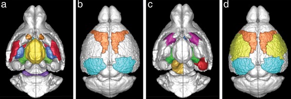
We combined all the subcortical regions from the Mori atlas and all the cortical parcellations from the NUS atlas (Fig. 1), by registering the NUS atlas T₂ image to the T₂ image of Mori atlas using a nonlinear registration called DRAMMS (Ou et al. 2011) to obtain the mouse connectome atlas with 42 ROIs that served as nodes in the connectivity matrix (21 on each hemisphere, see Supplementary Table 1). The combination of these 2 atlases facilitated maximum number of regions that could be utilized while covering majority of the brain areas that ultimately aided in describing the entire structural core of the mouse brain. These 42 ROIs were mapped to each subject using an affine registration (fsl-flirt) (Smith et al. 2004) followed by a nonlinear registration known as “deformable registration via attribute matching and mutual saliency weighting” or DRAMMS in short (Ou et al. 2011). DRAMMS registration uses multiscale and multiresolution Gabor attributes (which describe the texture) to find correspondence at each voxel, and uses the idea of mutual saliency weighting, wherein a metric is defined which assigns weights to different voxels quantifying the reliability of the correspondence.

Figure 1.

Creation of the connectivity atlas. (a) NUS atlas. (b) Mori atlas (note that the cortex is not parcellated in this atlas). (c) Registration using DRAMMS between NUS atlas T₂ image and Mori atlas T₂ image. (d) Cortical ROIs from NUS atlas transferred onto the Mori atlas while the subcortical ROIs from Mori atlas are retained and WM ROIs are removed. A total of 42 ROIs were used in creating the network.

For subjects with ages younger than day 15, the registration was carried out step-wise between the consecutive days, as a result of large growth. The deformation fields were concatenated to obtain the final field as was performed in (Baloch et al. 2009). The 42 regions defined in the atlas were then mapped onto each on the subject using the final deformation field. The evaluation of the registration was performed manually and the mapping of ROIs was checked for each subject as shown in the Supplementary Figure 1 that displays the mapped ROIs on a subjects of age days 40, 10, and 2.

Creating the Mouse Connectome

The mouse connectome was created based on number of fiber tracks computed between each pair of ROIs defined on the atlas, a schematic of which is presented in Figure 2. The DTI data were reconstructed using DTIStudio (Jiang et al. 2006). Deterministic full brain tractography was performed using Diffusion Toolkit and Trackvis (Wang and Van Wedeen 2007) using a stopping criteria of 0.1 FA and 35° curvature threshold (empirically chosen based on the ability to capture all the fibers at all time-points). The inter-regional connectivity between the 42 ROIs demarcated on the Mouse Connectome atlas was computed by applying the ROI masks to the reconstructed fiber tracks using the UCLA multimodal connectivity package (UMPC) (http://ccn.ucla.edu/wiki/index.php/UCLA_Multimodal_Connectivity_Package). This determined the number of tracks that originated in one ROI (i) and terminated in another ROI (j), for all possible pairs of 42 ROIs defined on the atlas, creating a 42 × 42 connectivity matrix W. This measure quantifies connectivity such that W_ij ≈ W_ji which on averaging gives an undirected weighted connectivity measure (Wang and van Wedeen 2007) as a part of standard connectivity matrix calculation. Since this matrix was computed in the subject space, the total number of fiber tracks as well as the size of ROI masks varied from subject to subject. The intersubject size differences were accounted for by normalizing the connectivity matrix by the total ROI volume of the 42 regions of that mouse. Usually, in human studies, the edge strength is not scaled by the brain volume or total ROI volume (Bassett et al. 2011). However, in our maturing mice dataset, brain size changed drastically and thus scaling the connectome using brain volume was crucial for group comparison. Also, alternate measures of connectivity can be adopted, however with the current scanning protocol and tractography the number of fibers is a better measure for the strength of connectivity between 2 ROIs.

Figure 2.

Pipeline for creating the mouse connectome.

An alternative measure like average FA of the tract could also be used, but such a measure gives an idea only of the WM integrity of the track whereas density of the track is the numbers of fibers that have endpoints present in the 2 ROIs under consideration quantifies the connectivity between those 2 ROIs. However, there is no ground truth for connectivity measures, and a similar analysis can be carried out by employing an alternate measure of choice.

Analysis of the Mouse Connectomes

The connectomes can be studied on a global level using several different network measures and on a local level, using network measures as well as on a connection-by-connection basis. While there are several biologically defined age sub-groups (pre- and postweaning; pre- and postpubertal), we investigated the maturation profile based on the changes that we observed via imaging. In the case of global measures, we investigated smaller age subgroups as the changes are expected to be highly nonlinear. For local measures and connection-wise analysis, the investigation was carried out in 2 subgroups: Group 1 (days 2–10) stage and group 2 (days 15–80) based on the developmental changes observed in prior imaging-based studies (Verma et al. 2005; Baloch et al. 2009), which showed a transition at day 10 in terms of changes in diffusion measures. Day 10 is also seen as an inflection point in the study of maturation patterns demonstrated via global network measures (discussed in Study of Density, Global Efficiency and Modularity with Age).

Local and Global Network Measures

The connectome can be analyzed at several levels of granularity using network measures that were developed to quantify networks in economics and biology. Of the numerous network measures (Rubinov and Sporns 2010), we present here 3 network measures that capture various aspects of the connectome and are shown to be important in developmental studies: density of the network as a basic measure, “global efficiency” as a robust measure of global integration, as well as “modularity” to quantify network segregation. In the context of brain networks, these measures are interpretable in terms of physiology, in contrast to some other graph theoretical measures. These network properties were computed using the brain connectivity toolbox (Rubinov and Sporns 2010) (http://www.brain-connectivity-toolbox.net/). The description of these measures is given below:

1. Density: The percentage of connections present related to a fully connected connectome.

2. Global efficiency: Global efficiency quantifies how well the regions communicate with each other, with shorter paths indicating a higher efficiency. (Here, shorter path defines purely the graph theoretical path length and is not related to the lengths of fibers.)

3. Modularity: Modularity reflects how well the network can be subdivided into nonoverlapping clusters or modules M (based on spectral clustering) (Newman 2006). A modularity measure (Q) of the community structure is based on the proportion of links connecting regions in different clusters.

   $$Q=\sum _{u\in M}\left[e_{uu}-{\left(\sum _{v\in M}{e}_{uv}\right)}^2\right].$$ (1)

   where e_uv is the proportion of all the edges that connect regions in module u with regions in module v. These modules (or clusters) (computed from the spectral clustering) can be compared for any of the 2 subjects by using adjusted mutual information (AMI) metric. The AMI ranges between 0 and 1, where 0 denotes no similarity between the clusters in subject 1 and 2 while AMI of 1 denotes exactly similar modules in both subjects.

All these global measures are examined via regression across the age span of the population.

Further, the local measures of degree and local efficiency are computed. These measures are defined at each node (i.e., each ROI) of the matrix. The details are given below:

1. Degree of region (node): The number of regions that are connected with a non-zero edge to that region (node).

2. Local efficiency of region (node): For region i, local efficiency is defined as the length of the shortest path between 2 regions that contains only the neighbors of i, where a_ijis the connection status between links i and j (is 0 with no link and 1 with link present), k is the degree of the node and d is the shortest path between 2 nodes.

$$E_{\mathrm{loc}}=\frac{1}{n}\sum _{i\in N}{E}_{\mathrm{loc},i}=\frac{1}{n}\sum _{i\in N}\frac{{\sum }_{j,h\in N,j\ne i}{a}_{ij}{a}_{ih}{[d_{jh}(N_i)]}^{-1}}{k_i(k_i-1)}.$$ (2)

These local measures were examined group-wise and the P-values computed from the Hotelling's t-statistic were corrected for multiple comparisons using Bonferroni (Dunnett 1964) correction (at 0.05).

Connection-Wise Analysis of the Connectome

After global and local analysis, we examined each of the connections of the connectome for group differences. Each connection W_ij was tested using Hotelling's t-test while linearly regressing out gender, and the resulting connection t-Statistic is used to construct the output T matrix (42 × 42). This T was then thresholded at positive and negative values to retain only those connections that were significantly stronger in either group. We used permutation testing on group labels (10 000 permutations) to address the problem of multiple comparisons implicit to this 42 × 42 hypothesis testing (Nichols and Holmes 2002). Using the maximum t-statistic at each of the 10 000 permutations, a histogram was constructed and a threshold value was computed at a significance level of P = 0.005. The connections with higher t-statistic value than the threshold were the ones that survived the correction.

Brain Connectivity Index

To distill this connectivity information down to a single index reflecting brain maturity from the perspective of connectivity, a machine-learning algorithm was used that employed the mouse connectomes to compute the BCI of the subject. In particular, using the connectomes as features and the logarithm of the age as a regressor, a support vector regression (SVR) (Vapnik 1998) model was created to train a connectomic age predictor of the subject (details given in Supplemetary material Section C). The log-age was used instead of the chronological age as the regressor as it is representative of the growth spurt in the early developmental days of the mice brain. A 10-fold cross-validation scheme was employed for the regression, in which the data were divided into 10 equal parts and one part was left out and the other 9 parts were used in training the SVR model. For attaining maximum generalization in the 10-fold process, we permuted the folds 10 times to obtain a comprehensive age prediction for each subject. This predicted age is referred as the BCI of the mouse. This was then correlated with the chronological age of the subject to determine how the brain maturation of the subject describes the real age and where it stands with respect to the population.

Results

Study of Density, Global Efficiency, and Modularity with Age

Global network measures were computed for the entire population and correlated with the chronological age. Figure 3 shows the high correlation of these network characteristics with age, where in the early postnatal days, the density and efficiency of the network is high and it drops as the mice mature up to day 10. After day 10, there is rapid increase till day 20, which plateaus in adulthood. On studying the maturation patterns, we see that 3 separate regression lines can be fitted to the data. The first line illustrates the early decline in density and efficiency of the network (days 2–10), and the second line (days 7–20) demonstrates the rapid increase, while the third line (days 15–80) represents the gradual increase, post the ages of 15–20 days.

Figure 3.

Change in global properties of the network with age. (a) Density, (b) global efficiency, and (c) modularity.

Modularity, on the other hand, shows a consistent increase as the mice mature. The rate of change is much higher in the earlier postnatal days that reduce as the mice reach adulthood. Therefore, modularity can be fitted using a nonlinear (logarithmic) function with respect to age (Fig. 3). Further, we investigated the modules membership of nodes (while computing modularity) and observed that the clustering was very similar between all the ages from days 2 to 15 (as calculated by AMI 0.43 ± 0.12), and within all the ages from days 20 to 80 (the AMI ranged from 0.40 ± 0.11). However, the clusters formed in subjects from days 2 to 15 displayed lower similarity to the clusters that were formed in older subjects (days 20–80), as demonstrated by low average AMI of 0.34 ± 0.07 (see Supplementary Fig. 2 showing the clustering similarity).

Changes in Nodal Measures with Age

An expected consequence of changes occurring in connection density between regions is that the degree of each region (represented as a node) varies with age. However, it is important to note that there is a differential increase/decrease in the degree of these nodes. That is, as the mouse brain develops, the degree of some regions increases/decreases rapidly but not in others, over the entire maturation span. The analysis of these measures was, therefore, carried out groupwise as described in Analysis of the Mouse Connectomes, based on where the imaging differences were seen in the past (Verma et al. 2005; Baloch et al. 2009). Figure 4a displays the ROIs whose degree increases significantly (P < 0.05, after Bonferroni correction) between the young and old groups while Figure 4b shows the regions where degree decreases significantly with maturation. Table 2 lists the regions with increased degree as the mice matured in age. The 2 groups could be changed based on where the global analysis above shows changes and inflection points.

Figure 4.

ROIs displaying significant changes in degree and local efficiency as the mice mature. (a) ROIs that demonstrated significantly higher degree in adult mice while (b) shows the ones with higher degree in younger mice. (c) ROIs that demonstrated significantly higher local efficiency in adult mice while (d) ROIs with higher local efficiency in younger mice. Note that, with maturation, the subcortical ROIs had higher degree and efficiency while, in cortical ROIs, reduced nodal features were observed.

Table 2.

List of regions that displayed significant change in degree and local efficiency between the 2 groups

Degree*	Local efficiency*
Older group > Younger group
1. Lateral globus pallidus (R and L)	1. Caudate and putamen (R and L)
2. Thalamus (R and L)	2. Superior colliculus (R)
3. Hypothalamus (R and L)	3. Thalamus (R and L)
4. Amygdala (R and L)	4. Septum (R and L)
5. Inferior colliculus (R and L)	5. Hippocampus (R and L)
6. Septum (R)
7. Accumbens (R and L)
8. Piriform cortex (R and L)
Younger group > Older group
1. Motor cortex (R and L)	1. Motor cortex (R and L)
2. Visual cortex (R and L)	2. Somatosensory cortex (R and L)
	3. Visual cortex (R and L)
	4. Lateral globus pallidus (L)

*P < 0.05 after Bonferroni correction.

Further analysis involving the local efficiency showed a heterogeneous increase between the ROIs, as was the case with the nodal degree. The regions that showed increased local efficiency (P < 0.05, after Bonferroni correction) are shown in Figure 4c and listed in Table 2. There was an increase in regional differences between the younger and the older group. Further, the young group demonstrated high efficiency in the cortical regions that involved somatosensory, motor, and visual cortex.

Connection-Wise Differences of the Mouse Connectome of the Developing Mouse Brain

Figure 5 shows the connection-wise differences between the 2 groups with P = 0.005 (after permutation testing). It can be observed that more than 20% of the subcortical connections have significantly higher connection strength in the older group when compared with the younger mice (yellow edges). For example, connections from thalamus to other subcortical regions like septum, hippocampus, hypothalamus, and globus pallidus increased significantly with age. In Figure 5, the connections in blue indicate those that were significantly higher in younger mice than the older mice. These connections include mainly cortical–cortical connections like retro-splenial granular, somatosensory, and piriform cortex, connecting to the motor cortex. Some connections between the hippocampus and the cortex were also found to be significantly higher in younger group. No significant effects were seen between the 2 genders as no edges survived significance of P < 0.005.

Figure 5.

Connection-wise differences between the 2 groups. Blue edges indicate significantly higher connectivity in younger group and yellow edges indicate significantly higher connectivity in adult group. The cortical regions are indicated by green dots while subcortical regions are displayed with red dots. Significance is defined at P-value of <0.005 after permutation testing.

Brain Connectivity Index

Figure 6 shows the prediction of age based on our SVR model trained on the mouse connectomes. The resulting correlation between the chronological age and BCI was high (r = 0.95). The dotted line in Figure 6 depicts the ideal correlation of 100%, while the solid line is the predicted correlation. Note that Figure 6 displays the predicted age (after computing the exponential of the log-age) plotted against the chronological age (x-axis).

Figure 6.

Multivariate SVR trained on the mouse connectomes to obtain the BCI of each subject in the population (y-axis). This was highly correlated with the chronological age (x-axis) of the mouse. The dotted line depicts 100% correlation, while the solid line shows the actual correlation (0.95).

Discussion

The work presented here is unique as it creates a mouse connectome using high-resolution DTI. A connectome quantifies the full brain connectivity network incorporating information from all the cortical and subcortical pathways, and is commonly created on human brains. In this context, our mouse connectome can potentially be an important model for future mouse studies, to understand neurological and psychiatric disorders that involve genetic alteration or environmental manipulation. In this article, we created a connectomic profile of mouse brain maturation in the early postnatal period (days 2–80) to characterize dynamic patterns of change during development. Measures were based on the structure of the connectomes, as well as connection-wise statistics that provided insight into the processes of myelin and axonal maturation and dendritic tree elaboration in the mouse brain.

The analysis was carried out at various levels—ranging from inter-regional connections, to measures that quantify the local and global connectivity, for investigating the maturation profile based on ages at which the imaging changes have been observed. So, while the data can be biologically grouped into several groups based on weaning and puberty, we tried to investigate the maturation in terms of what was evident from the imaging. Ideally, the analysis should be done without any imposed groupings, as was undertaken in the analysis of the global measures of density, global efficiency, and modularity. These measures provided an insight into the connectomic maturation profile at a macroscopic level. Density and efficiency displayed a complex pattern during development while modularity showed a nonlinear (logarithmic) increase with age (Fig. 4). The investigation of local and connection-wise analysis would be considerably more challenging to interpret without introducing the grouping, as the measures were at the level of each node and each pair-wise connection, respectively and it was difficult to query each node/edge independently. As such, we divided the population into 2 groups—before and after day 10, where the imaging changes have been observed (Baloch et al. 2009) and biologically it corresponds to eyes closed state (days 2–10) and eyes open state (after day 15). The local measures captured the heterogeneity in developmental changes in connectivity via 2 local features: degree and local efficiency. Next, at the level of connections, the statistical analysis between the 2 groups displayed higher strength in cortical connections (P < 0.005 after 10 000 permutations) in the younger mice, while the older mice demonstrated higher strength in subcortical connections (P < 0.005 after 10 000 permutations).

All the results (global, local, and connection-wise) suggest that the process of maturation may involve a combination of dendritic pruning and axonal maturation, which cannot always be teased apart. From Figure 3, it can be seen that, at a very young age (days 2 and 3), the density and the global efficiency of the network were high compared with the ages between days 5 and 10. This is potentially a manifestation of the cortical gray matter being highly anisotropic at days 2 and 3 due to a neuronal migration along the radial glial scaffolding (Verma et al. 2005; Huppi and Dubois 2006). The brain architecture is dominated by these cortico-radial fibers and by the radially orientated apical dendrites of pyramidal cells (Mukherjee and McKinstry 2006). This radial orientation of the dendrites provides directionality for water diffusion, causing the tensors to be oriented in the radial direction to the cortical surface, which consequently leads to higher connection density between adjacent cortical regions (as seen in Fig. 5). This in turn increases the overall network density, as well as the global efficiency of the network. This is specifically observed in motor and visual cortex via degree and local efficiency being higher in the younger group. However, with an increase in age (between days 5 and 10), the neocortex starts maturing with transformation of the radial glia into the more complex astrocytic neurophil, and the addition of basal dendrites that disrupts the cortical architecture as these are orthogonal to the apical dendrites thus reducing the density of the network. After day 10, anisotropy in the WM increases, suggesting an increase in axonal packing and myelination. Pathways like the ventral hippocampal commissure, the internal and external capsule, and the corpus callosum became denser, forming more links between the subcortical structures (Verma et al. 2005; Chuang et al. 2011). This results in a larger number of regions getting interconnected, forming a denser network, thereby increasing the network density. The maturation is rapid until day 20 (Fig. 3) and then proceeds more gradually. This phenomenon is also observed in the connection-wise results, where subcortical regions have significantly higher number of connections in the older group (Fig. 5), as well as in the nodal features where structures like the thalamus, amygdala, and hypothalamus displayed high degree and local efficiency in the older group. The behavior of the changes in network density and global efficiency with age required the fitting of 3 regression lines (from days 2–10, days 7–20, and days 15–80; Fig. 3), as the single linear regression model could not characterize the variable changes. Overlapping lines were fitted in order to capture the entire developmental spectrum. The regression line from days 2 to 10 characterizes the maturation in cortex while regression lines fitted to ages from 7–20 and 15–80, respectively potentially characterizes the increase in axonal packing and myelination in WM tissue. (McKinstry et al. 2002; Yoshida et al. 2013).

The increase in WM integrity after day 10 can also be related to the beginning of the “critical period” in mice. After eye opening, the mice perceive visual signals that aid in brain maturation. This phenomenon is described as ocular dominance plasticity of the brain and has been studied thoroughly in rodents and cats (Dudek and Bear 1989; Fagiolini et al. 1994). Thus, the fiber tracts that were relatively underdeveloped in the early postnatal days (eyes closed), matured rapidly to connect more regions and then reached a steady state (around day 40 – end of “critical period”). It is important to note that the cortical maturation after day 7 can only be captured via diffusivity indices; it cannot be captured through fiber tracking as the gray matter becomes highly isotropic as the mice mature, and tracking is not reliable in low anisotropy regions. However, in future, measures like diffusivity could be included in the connectome creation to incorporate this information. These results are similar to those from studies on human brain development, that have shown increased connection strengths (Hagmann et al. 2010; Dennis et al. 2013) potentially arising from axonal maturation, as well as myelination and is demonstrated via increase in FA in WM by the majority of neonatal/pediatric DTI studies (Huppi and Dubois 2006; Mukherjee and McKinstry 2006; Yoshida et al. 2013). The radial organization of the cortex has been illustrated in some studies using FA and radial diffusivity changes (McKinstry et al. 2002; Yoshida et al. 2013).

Modularity is the ability of the network to be divided into clusters. The modularity of the network is a feature that underlines the community structure of the network, while measuring the segregation. Modularity of the developing mice brains demonstrated a logarithmic increase with age (Fig. 3; r = 0.73). In young mice, the brain network was relatively nonmodular; however with maturation, the modularity increased rapidly till it plateaued (Fair et al. 2009). This potentially indicates neuronal plasticity that allows the brain to go through a reorganization in response to environmental stimulation, optimizing the necessary connections to maximize the network performance and minimize the connection cost (Kentroti and Vernadakis 1990; Johnston 2009; Kolb and Gibb 2011). Further, on analyzing the resulting modules based on the AMI index (as described in Study of Density, Global Efficiency and Modularity with Age), it was observed that the modular structure of the mouse brain underwent major reorganization after the age of day 15. The module membership of the regions was similar between all the ages of days 2–15 and from days 20 to 80. However, the clustering (or modules) between early postnatal days (2–15 days) and the later days (days 20–80) displayed lower similarity (see Supplementary Fig. 2). This possibly explains the major brain changes that occur after day 18 as shown through behavioral and memory tests in mice (Rudy and Morledge 1994). Also, this observation agrees with the study from Fair et al. (2009) on human brains between children and young adults using functional connectomes.

Finally, with the aim of quantifying the location of each mouse over the developmental spectrum, based on the level of brain maturation, we designed the concept of BCI, which provides a phenotypic measure of maturation. BCI showed a very high (r = 0.95) correlation with the chronological age. This implies that the connectome was a good representative of the actual age of a normative mouse. Any change induced by pathology, as in the case of mutant mice, would cause connectomic age to differ from the normative age, helping to identify outliers that could be further investigated. For example, in mutant mouse models of schizophrenia (for example, neuregulin knockouts), the connectomic age is expected to be lower than the actual age. While in mouse models of autism (protocadherin-10 knockouts), due to an increase in short range connectivity, we expect there to be growth spurt and a slow-down, causing the brains to display such a behavior in terms of the connectomic age.

Human studies on brain development that employ DTI-based connectomic analysis have not been applied to study developmental changes from in utero, or early postnatal days. For example, in the study by Hagmann et al. (2010), the youngest subjects were 2 years old while, in other studies, the youngest age ranged from 12 to 20 years (Gong et al. 2009; Dennis et al. 2013). Employing human pediatric or neonatal data in connectivity analysis is challenging as the gray-matter regions vary significantly during the course of development due to high gyrification and maturation during this period. Nevertheless, one recent study by Yap et al. (2011) employed pediatric data from 2-week-old subjects, 1-year, and 2-year olds, and demonstrated an increase in modularity with development. However, in such human studies, it is very important to take into account the noise that originates from babies moving in the scanner or inutero, as that can significantly alter the results. In the case of our ex vivo mouse brains, the output images were high resolution, with a high SNR and enabled us to study brain development from very early postnatal days. This mouse developmental trajectory could be utilized as a baseline for studies evaluating the effect of genetic modifications, as these are commonly carried out in the mouse to model neurological deficits and psychiatric disorders.

Computing imaging-based structural brain connectome requires well-defined anatomical regions of interest, both cortical and subcortical. In studies involving human MRI, a variety of templates (e.g., AAL atlas, Desikan atlas) have been created to this date and can be applied effortlessly for computing the connectivity (Desikan et al. 2006). On the contrary, the mouse atlases defined on MRI data either do not encompass the entire brain (some parts of the brain are not defined) or contain fewer regions of interest (coarse parcellation). Furthermore, developmental atlases defined contain structures segmented at various developmental time-points that do not allow group-wise analysis as the connectomes may not be comparable across ages. This underlines the need for create an atlas of the mouse brain that contained well-defined cortical parcellations and subcortical structures. Our work took a step forward by combining the NUS atlas (Bai et al. 2012) and the Mori atlas (Chuang et al. 2011) (Fig. 2) using accurate nonlinear registration between the 2, to create an atlas of the mouse brain. We plan to release this atlas in the near future such that it can be used by the neuroimaging community as well as aid future mouse connectomic studies. While creating the normative connectomic atlas of mouse brains is a representative study and indicates how connectomic studies can be carried out in the future, this atlas can be used as a baseline to study changes in mutant mice.

The data were acquired with only 6 directions to keep a low acquisition time, limiting a tensor fit to the data. The number of gradient directions was traded for a scan with high spatial resolution, as well as high SNR, by repeating the scan 7 times. The scanning protocol for this study was planned before higher b-value acquisitions could be acquired in a short time. For the purpose of maintaining consistency, the acquisition protocol was not changed. Less number of gradient directions may introduce a bias as shown by Jones (2003); therefore, future studies are required to understand the effect of gradients on the network structure. However, with the increased spatial resolution of a less complex mouse brain, we expected to and have been able to obtain a fair insight into the WM microstructure, even with a tensor fit to the data. With enhanced imaging capabilities, in future, we expect to acquire high angular resolution diffusion data. A perceived limitation could be uncontrolled litter sizes, leading to differences in brain volume. Also younger mice were scanned within the skull to avoid nicks and cuts in the brain. In order to account for the swelling and deformation arising from these sources, we normalized each of the connectivity matrices by dividing by the total regional volume (proportional to brain volume) of the seed. Also, as all the younger animals have been treated similarly, we expect that the more troubling within-day bias was alleviated.

Our maturation dataset involved mice from days 2 to 80, and therefore registering the ROIs from the atlas to the younger mice was a complex task. We chose the method known as DRAMMS and employed a step-wise registration for mice below day 15. DRAMMS registration extracts multiscale and multiresolution Gabor attributes (which describe the texture) at each voxel. Compared with the traditionally used intensity features, texture attribute matching is precise as each voxel is more distinctive and therefore finding correspondences is more accurate. Further, DRAMMS uses the idea of mutual saliency weighting, where a metric is defined which assigns different weights to different voxels based on how reliable the correspondence in the other image is. Therefore, DRAMMS was a favorable choice for registering developing mouse brains, as the intensity in the FA images of the mouse brains changes based on age and therefore the similarity metric based on texture features (Gabor features) is more suitable. Also, for missing correspondences (e.g., underdeveloped regions in younger mice in our case), the automatically computed mutual saliency weighting drives the registration to be more accurate. Thus, even though younger mice may have underdeveloped regions of interest, the registration could perform well in these regions. Additionally, the 42 regions defined on the atlas were gross regions (see Supplementary Table 1) and therefore DRAMMS could conform to the nonlinear size and shape changes of these big structures with acceptable accuracy (see Supplementary Fig. 1 that illustrates the quality of registration by displaying the ROIs mapped onto days 40, 10, and 2). Also, all these regions are present in the youngest of the mice as shown by Foster histological atlas (Foster 1998). We employed deterministic whole-brain tracking on all the mice while retaining the same parameters. The connectome alternatively can be computed by using various available tracking algorithms; however, the effect of tractography on the network needs to be addressed in future.

Finally, we chose the number of fibers scaled by the brain volume as the measure of connection between the 2 regions. While the number of fibers depicts the brain wiring between the 2 regions, it is not the actual number of axonal measures. This number is highly dependent upon the tractography algorithm as well as the parameters chosen. However, with consistent tracking on all subjects, with the same parameters, we believe that the number of fibers is a good choice. This is not a measure of the underlying integrity of the WM as axonal density is. In the future, connectomes could be created using a combination of connectivity and integrity and, in those cases, measures of axonal quality like axonal density could be used (Alexander et al. 2010). This would require a multishell HARDI acquisition, which is beyond the scope of this paper and a possibility for future work (Alexander et al. 2010).

In summary, this paper lays the foundation for imaging-based structural connectomics of the mouse brain by creating a structural mouse connectome using diffusion imaging. The connectomic atlas provided along with the connectome (will be released on http://www.rad.upenn.edu/sbia/ in near future) facilitates the creation and comprehensive characterization of the whole-brain network leading to population-based studies on connectivity. A normative connectomic trajectory of maturation during postnatal ages 2–80 days is presented in the C57BL/6J mouse strain, using a full brain connectivity analysis, followed by investigations based on local and global network features. The global network measures of density and global efficiency presented complex patterns of change with age while modularity demonstrated a nonlinear relationship with age, indicating an enhanced change in the early days of the maturation trajectory. In future, we plan on validating our DTI-based connectome against the Allen brain atlas connectome—a detailed tracer-based connectome (Lein et al. 2007) in adult mice. Also, we plan on utilizing the hybridization data provided by the Allen brain atlas for correlation of genetic effects against the connectome.

This work quantifies the brain changes in connectivity during development, and can be employed to study deviations from it related to genetic and environmental effects. We expect that this will be used as a normative baseline for studies of mutant mice. Finally, BCI, with its high correlation with chronological age is established as a robust phenotypic marker of age progression valuable in detecting subtle deviations from normality caused by genetic mutations.

Supplementary Material

Supplementary material can be found at: http://www.cercor.oxfordjournals.org/

Funding

This work was supported by National Institute of Health grants RO1-MH-070365 and R01-MH079938.

References

- Aggarwal M, Duan W, Hou Z, Rakesh N, Peng Q, Ross CA, Miller MI, Mori S, Zhang J. 2012. Spatiotemporal mapping of brain atrophy in mouse models of Huntington's disease using longitudinal in vivo magnetic resonance imaging. Neuroimage. 60(4):2086–2095. [DOI] [PMC free article] [PubMed] [Google Scholar]
- Alexander DC, Hubbard PL, Hall MG, Moore EA, Ptito M, Parker GJ, Dyrby TB. 2010. Orientationally invariant indices of axon diameter and density from diffusion MRI. Neuroimage. 52(4):1374–1389. [DOI] [PubMed] [Google Scholar]
- Assaf Y, Galron R, Shapira I, Nitzan A, Blumenfeld-Katzir T, Solomon AS, Holdengreber V, Wang Z-Q, Shiloh Y, Barzilai A. 2008. MRI evidence of white matter damage in a mouse model of Nijmegen breakage syndrome. Exp Neurol. 209(1):181–191. [DOI] [PubMed] [Google Scholar]
- Bai J, Trinh TL, Chuang KH, Qiu A. 2012. Atlas-based automatic mouse brain image segmentation revisited: model complexity vs. image registration. Magn Reson Imaging. 30(6):789–798. [DOI] [PubMed] [Google Scholar]
- Baloch S, Verma R, Huang H, Khurd P, Clark S, Yarowsky P, Abel T, Mori S, Davatzikos C. 2009. Quantification of brain maturation and growth patterns in C57BL/6J mice via computational neuroanatomy of diffusion tensor images. Cereb Cortex. 19(3):675–687. [DOI] [PMC free article] [PubMed] [Google Scholar]
- Bassett DS, Brown JA, Deshpande V, Carlson JM, Grafton ST. 2011. Conserved and variable architecture of human white matter connectivity. Neuroimage. 54(2):1262–1279. [DOI] [PubMed] [Google Scholar]
- Bullmore E, Sporns O. 2009. Complex brain networks: graph theoretical analysis of structural and functional systems. Nat Rev Neurosci. 10(3):186–198. [DOI] [PubMed] [Google Scholar]
- Bullmore ET, Bassett DS. 2010. Brain graphs: graphical models of the human brain connectome. Annu Rev Clin Psychol. 7:113–140. [DOI] [PubMed] [Google Scholar]
- Chuang N, Mori S, Yamamoto A, Jiang H, Ye X, Xu X, Richards LJ, Nathans J, Miller MI, Toga AW, et al. 2011. An MRI-based atlas and database of the developing mouse brain. Neuroimage. 54(1):80–89. [DOI] [PMC free article] [PubMed] [Google Scholar]
- Dennis EL, Jahanshad N, McMahon KL, de Zubicaray GI, Martin NG, Hickie IB, Toga AW, Wright MJ, Thompson PM. 2013. Development of brain structural connectivity between ages 12 and 30: a 4-Tesla diffusion imaging study in 439 adolescents and adults. Neuroimage. 64:671–684. [DOI] [PMC free article] [PubMed] [Google Scholar]
- Desikan RS, Segonne F, Fischl B, Quinn BT, Dickerson BC, Blacker D, Buckner RL, Dale AM, Maguire RP, Hyman BT, et al. 2006. An automated labeling system for subdividing the human cerebral cortex on MRI scans into gyral based regions of interest. Neuroimage. 31(3):968–980. [DOI] [PubMed] [Google Scholar]
- Dudek SM, Bear MF. 1989. A biochemical correlate of the critical period for synaptic modification in the visual cortex. Science. 246(4930):673–675. [DOI] [PubMed] [Google Scholar]
- Dunnett CW. 1964. New tables for multiple comparisons with control. Biometrics. 20(3):482–491. [Google Scholar]
- Ellegood J, Lerch JP, Henkelman RM. 2011. Brain abnormalities in a Neuroligin3 R451C knockin mouse model associated with autism. Autism Res. 4(5):368–376. [DOI] [PubMed] [Google Scholar]
- Ellegood J, Pacey LK, Hampson DR, Lerch JP, Henkelman RM. 2010. Anatomical phenotyping in a mouse model of fragile X syndrome with magnetic resonance imaging. Neuroimage. 53(3):1023–1029. [DOI] [PubMed] [Google Scholar]
- Fagiolini M, Pizzorusso T, Berardi N, Domenici L, Maffei L. 1994. Functional postnatal development of the rat primary visual cortex and the role of visual experience: dark rearing and monocular deprivation. Vision Res. 34(6):709–720. [DOI] [PubMed] [Google Scholar]
- Fair DA, Cohen AL, Power JD, Dosenbach NU, Church JA, Miezin FM, Schlaggar BL, Petersen SE. 2009. Functional brain networks develop from a "local to distributed" organization. PLoS Comput Biol. 5(5):e1000381. [DOI] [PMC free article] [PubMed] [Google Scholar]
- Foster G. 1998. Chemical neuroanatomy of the prenatal rat brain, a developmental atlas. Oxford: Oxford University Press. [Google Scholar]
- Gong G, Rosa-Neto P, Carbonell F, Chen ZJ, He Y, Evans AC. 2009. Age- and gender-related differences in the cortical anatomical network. J Neurosci. 29(50):15684–15693. [DOI] [PMC free article] [PubMed] [Google Scholar]
- Grabill C, Silva AC, Smith SS, Koretsky AP, Rouault TA. 2003. MRI detection of ferritin iron overload and associated neuronal pathology in iron regulatory protein-2 knockout mice. Brain Res. 971(1):95–106. [DOI] [PubMed] [Google Scholar]
- Gutman DA, Keifer OP, Jr, Magnuson ME, Choi DC, Majeed W, Keilholz S, Ressler KJ. 2012. A DTI tractography analysis of infralimbic and prelimbic connectivity in the mouse using high-throughput MRI. Neuroimage. 63(2):800–811. [DOI] [PMC free article] [PubMed] [Google Scholar]
- Hagmann P, Cammoun L, Gigandet X, Meuli R, Honey CJ, Wedeen VJ, Sporns O. 2008. Mapping the structural core of human cerebral cortex. PLoS Biol. 6(7):e159. [DOI] [PMC free article] [PubMed] [Google Scholar]
- Hagmann P, Sporns O, Madan N, Cammoun L, Pienaar R, Wedeen VJ, Meuli R, Thiran JP, Grant PE. 2010. White matter maturation reshapes structural connectivity in the late developing human brain. Proc Natl Acad Sci USA. 107(44):19067–19072. [DOI] [PMC free article] [PubMed] [Google Scholar]
- Harsan LA, Paul D, Schnell S, Kreher BW, Hennig J, Staiger JF, von Elverfeldt D. 2010. In vivo diffusion tensor magnetic resonance imaging and fiber tracking of the mouse brain. NMR Biomed. 23(7):884–896. [DOI] [PubMed] [Google Scholar]
- Huppi PS, Dubois J. 2006. Diffusion tensor imaging of brain development. Semin Fetal Neonatal Med. 11(6):489–497. [DOI] [PubMed] [Google Scholar]
- Jiang H, van Zijl PCM, Kim J, Pearlson GD, Mori S. 2006. DtiStudio: resource program for diffusion tensor computation and fiber bundle tracking. Comput Methods Programs Biomed. 81(2):106–116. [DOI] [PubMed] [Google Scholar]
- Johnston MV. 2009. Plasticity in the developing brain: implications for rehabilitation. Dev Disabil Res Rev. 15(2):94–101. [DOI] [PubMed] [Google Scholar]
- Jones DK. 2003. Determining and visualizing uncertainty in estimates of fiber orientation from diffusion tensor MRI. Magn Reson Med. 49(1):7–12. [DOI] [PubMed] [Google Scholar]
- Kentroti S, Vernadakis A. 1990. Neuronal plasticity in the developing chick brain: interaction of ethanol and neuropeptides. Brain Res Dev Brain Res. 56(2):205–210. [DOI] [PubMed] [Google Scholar]
- Kolb B, Gibb R. 2011. Brain plasticity and behaviour in the developing brain. J Can Acad Child Adolesc Psychiatry. 20(4):265–276. [PMC free article] [PubMed] [Google Scholar]
- Kooy RF, Reyniers E, Verhoye M, Sijbers J, Bakker CE, Oostra BA, Willems PJ, Van Der Linden A. 1999. Neuroanatomy of the fragile X knockout mouse brain studied using in vivo high resolution magnetic resonance imaging. Eur J Hum Genet. 7(5):526–532. [DOI] [PubMed] [Google Scholar]
- Kovacevic N, Henderson JT, Chan E, Lifshitz N, Bishop J, Evans AC, Henkelman RM, Chen XJ. 2005. A three-dimensional MRI atlas of the mouse brain with estimates of the average and variability. Cereb Cortex. (New York, N Y: 1991). 15(5):639–645. [DOI] [PubMed] [Google Scholar]
- Larvaron P, Boespflug-Tanguy O, Renou J-P, Bonny J-M. 2007. In vivo analysis of the post-natal development of normal mouse brain by DTI. NMR Biomed. 20(4):413–421. [DOI] [PubMed] [Google Scholar]
- Lein ES, Hawrylycz MJ, Ao N, Ayres M, Bensinger A, Bernard A, Boe AF, Boguski MS, Brockway KS, Byrnes EJ, et al. 2007. Genome-wide atlas of gene expression in the adult mouse brain. Nature. 445(7124):168–176. [DOI] [PubMed] [Google Scholar]
- McDaniel B, Sheng H, Warner DS, Hedlund LW, Benveniste H. 2001. Tracking brain volume changes in C57BL/6J and ApoE-deficient mice in a model of neurodegeneration: a 5-week longitudinal micro-MRI study. Neuroimage. 14(6):1244–1255. [DOI] [PubMed] [Google Scholar]
- McKinstry RC, Mathur A, Miller JH, Ozcan A, Snyder AZ, Schefft GL, Almli CR, Shiran SI, Conturo TE, Neil JJ. 2002. Radial organization of developing preterm human cerebral cortex revealed by non-invasive water diffusion anisotropy MRI. Cereb Cortex. 12(12):1237–1243. [DOI] [PubMed] [Google Scholar]
- Moldrich RX, Pannek K, Hoch R, Rubenstein JL, Kurniawan ND, Richards LJ. 2010. Comparative mouse brain tractography of diffusion magnetic resonance imaging. Neuroimage. 51(3):1027–1036. [DOI] [PMC free article] [PubMed] [Google Scholar]
- Mori S, Itoh R, Zhang J, Kaufmann WE, van Zijl PC, Solaiyappan M, Yarowsky P. 2001. Diffusion tensor imaging of the developing mouse brain. Magn Reson Med. 46(1):18–23. [DOI] [PubMed] [Google Scholar]
- Mukherjee P, McKinstry RC. 2006. Diffusion tensor imaging and tractography of human brain development. Neuroimaging Clin N Am. 16(1):19–43, vii. [DOI] [PubMed] [Google Scholar]
- Munasinghe JP, Gresham GA, Carpenter TA, Hall LD. 1995. Magnetic resonance imaging of the normal mouse brain: comparison with histologic sections. Lab Anim Sci. 45(6):674–679. [PubMed] [Google Scholar]
- Newman MEJ. 2006. Modularity and community structure in networks. Proc Natl Acad Sci USA. 103(23):8577–8582. [DOI] [PMC free article] [PubMed] [Google Scholar]
- Nichols TE, Holmes AP. 2002. Nonparametric permutation tests for functional neuroimaging: a primer with examples. Hum Brain Mapp. 15(1):1–25. [DOI] [PMC free article] [PubMed] [Google Scholar]
- Nieman BJ, Bock NA, Bishop J, Chen XJ, Sled JG, Rossant J, Henkelman RM. 2005. Magnetic resonance imaging for detection and analysis of mouse phenotypes. NMR Biomed. 18(7):447–468. [DOI] [PubMed] [Google Scholar]
- Ou Y, Sotiras A, Paragios N, Davatzikos C. 2011. DRAMMS: deformable registration via attribute matching and mutual-saliency weighting. Med Image Anal. 15(4):622–639. [DOI] [PMC free article] [PubMed] [Google Scholar]
- Pierpaoli C, Jezzard P, Basser PJ, Barnett A, Di Chiro G. 1996. Diffusion tensor MR imaging of the human brain. Radiology. 201(3):637–648. [DOI] [PubMed] [Google Scholar]
- Rubinov M, Sporns O. 2010. Complex network measures of brain connectivity: uses and interpretations. Neuroimage. 52(3):1059–1069. [DOI] [PubMed] [Google Scholar]
- Rudy JW, Morledge P. 1994. Ontogeny of contextual fear conditioning in rats: implications for consolidation, infantile amnesia, and hippocampal system function. Behav Neurosci. 108(2):227–234. [DOI] [PubMed] [Google Scholar]
- Sizonenko SV, Camm EJ, Garbow JR, Maier SE, Inder TE, Williams CE, Neil JJ, Huppi PS. 2007. Developmental changes and injury induced disruption of the radial organization of the cortex in the immature rat brain revealed by in vivo diffusion tensor MRI. Cereb Cortex. 17(11):2609–2617. [DOI] [PMC free article] [PubMed] [Google Scholar]
- Smith SM, Jenkinson M, Woolrich MW, Beckmann CF, Behrens TEJ, Johansen-Berg H, Bannister PR, De Luca M, Drobnjak I, Flitney DE, et al. 2004. Advances in functional and structural MR image analysis and implementation as FSL. Neuroimage. 23(Suppl 1):S208–S219. [DOI] [PubMed] [Google Scholar]
- Song SK, Yoshino J, Le TQ, Lin SJ, Sun SW, Cross AH, Armstrong RC. 2005. Demyelination increases radial diffusivity in corpus callosum of mouse brain. Neuroimage. 26(1):132–140. [DOI] [PubMed] [Google Scholar]
- Spencer NG, Bridges LR, Elderfield K, Amir K, Austen B, Howe FA. 2013. Quantitative evaluation of MRI and histological characteristics of the 5xFAD Alzheimer mouse brain. Neuroimage. 76:108–115. [DOI] [PubMed] [Google Scholar]
- Sporns O. 2011. The human connectome: a complex network. Ann N Y Acad Sci. 1224:109–125. [DOI] [PubMed] [Google Scholar]
- Vapnik VN. 1998. Statistical learning theory. New York: Wiley. [DOI] [PubMed] [Google Scholar]
- Verma R, Mori S, Shen D, Yarowsky P, Davatzikos C. 2005. Spatio-temporal maturation patterns of murine brain quantified via diffusion tensor MRI and deformation-based morphometry. Proc Natl Acad Sci. 102(19):6978–6983. [DOI] [PMC free article] [PubMed] [Google Scholar]
- Wang R, Van Wedeen J. 2007. Diffusion toolkit: a software package for diffusion imaging data processing and tractography. Trackvis.org. Martinos Center for Biomedical Imaging. Massachusetts General Hospital. [Google Scholar]
- Yap PT, Fan Y, Chen Y, Gilmore JH, Lin W, Shen D. 2011. Development trends of white matter connectivity in the first years of life. PLoS One. 6(9):e24678. [DOI] [PMC free article] [PubMed] [Google Scholar]
- Yoshida S, Oishi K, Faria AV, Mori S. 2013. Diffusion tensor imaging of normal brain development. Pediatr Radiol. 43(1):15–27. [DOI] [PMC free article] [PubMed] [Google Scholar]
- Zhang J, Peng Q, Li Q, Jahanshad N, Hou Z, Jiang M, Masuda N, Langbehn DR, Miller MI, Mori S, et al. 2010. Longitudinal characterization of brain atrophy of a Huntington's disease mouse model by automated morphological analyses of magnetic resonance images. Neuroimage. 49(3):2340–2351. [DOI] [PMC free article] [PubMed] [Google Scholar]
- Zhang J, Richards LJ, Miller MI, Yarowsky P, van Zijl P, Mori S. 2006. Characterization of mouse brain and its development using diffusion tensor imaging and computational techniques. Conf Proc IEEE Eng Med Biol Soc. 1:2252.–. [DOI] [PubMed] [Google Scholar]
- Zhang J, Richards LJ, Yarowsky P, Huang H, van Zijl PCM, Mori S. 2003. Three-dimensional anatomical characterization of the developing mouse brain by diffusion tensor microimaging. Neuroimage. 20(3):1639–1648. [DOI] [PubMed] [Google Scholar]
Associated Data
This section collects any data citations, data availability statements, or supplementary materials included in this article.