Integrating Single-Molecule Experiments and Discrete Stochastic Models to Understand Heterogeneous Gene Transcription Dynamics

Abstract

The production and degradation of RNA transcripts is inherently subject to biological noise that arises from small gene copy numbers in individual cells. As a result, cellular RNA levels can exhibit large fluctuations over time and from one cell to the next. This article presents a range of precise single-molecule experimental techniques, based upon RNA fluorescence in situ hybridization, which can be used to measure the fluctuations of RNA at the single-cell level. A class of models for gene activation and deactivation is postulated in order to capture complex stochastic effects of chromatin modifications or transcription factor interactions. A computational tool, known the Finite State Projection approach, is introduced to accurately and efficiently analyze these models in order to predict how probability distributions of RNA change over time in response to changing environmental conditions. These single-molecule experiments, discrete stochastic models, and computational analyses are systematically integrated to identify models of gene regulation dynamics. To illustrate the power and generality of our integrated experimental and computational approach, we explore cases that include different models for three different RNA types (sRNA, mRNA and nascent RNA), three different experimental techniques and three different biological species (bacteria, yeast and human cells).

1. Introduction

In recent years, advanced experimental techniques have provided biologists with unprecedented abilities to probe and observe the myriad parts of biological processes. Techniques such as RNA sequencing, super-resolution fluorescent imaging, and flow-cytometry have provided details of individual biological components, even at single-cell and single-molecule resolutions [1, 2, 3, 4]. Such detailed observations have largely out-paced our ability to understand, interpret, predict or influence these processes. A key contributor to the disconnect between the availability of high-throughput biological data and quantitative, predictive biological understanding is the extremely complex and often random nature of biological systems. Large numbers of chemical species all interact in complex, non-linear networks to carry out even the most basic biological tasks, such as transcription regulation. Furthermore, inherent in any experimentally observed biological system are several types of “noise”, including intrinsic fluctuations in cellular constituents, extrinsic heterogeneities between cells, measurement inaccuracies, and inadvertent environmental fluctuations. When these complex processes and unavoidable noise combine together, the result may make it extremely difficult to match or predict biological phenomena.

Mathematical modeling of biological systems can serve a variety of purposes, such that different models may satisfy different goals. The goal of some models may be to create a comprehensive representation of a biological process by compiling all known understanding of that particular system [5, 6]. While such models are qualitative in nature, they can provide a complete picture of how a particular system is currently understood to behave and can be used to test broad qualitative hypotheses. Conversely, the goal of conceptual models may be to capture a small part of larger biological networks, or to reveal physical principles about how an individual subsystem behaves in specific circumstances [7, 8]. In this article, we investigate a third goal of modeling: to quantitatively predict how a system will behave under experimental conditions. Where comprehensive models may be complex combinations of hundreds of reactions and biophysical parameters, and principle based models may be exceptionally simple, in optimally predicting models, the complexity is dictated by existing quantitative data and predictive goals [9]. Uncertainty from measurement noise combined with highly complex biological systems may lead to poor parameter identification and a resulting loss in predictive power. Two questions naturally arise: how do the challenges presented by biological complexity restrict predictive modeling and in what ways can emerging experimental approaches enable improved predictive understanding?

The first such challenge of model identification is “model sloppiness”–the notion that parameters are often poorly constrained, especially in biological models [10]. For a given amount and type of experimental data, only certain parameter combinations will be well defined, leading to large regions of parameter uncertainty. Moreover, addition of more data of the same type may fail to reduce the parameter uncertainties. This diminishing return from additional data motivates a need for enhanced experiments that complement models or reduced models that complement the available data. In some fortuitous cases, additional data may already exist that has not yet been fully utilized. For example, fitting deterministic models (i.e., sets of ordinary differential equations, or ODEs) to single-cell distributions may partially constrain parameters, but often ignoring cell-to-cell heterogeneity may limit success in model identification [11]. In other words, biochemical noise, the fluctuations inherent to the biological process being measured, may provide information inaccessible when measured with bulk analysis (e.g., PCR or western blot analysis of RNA or protein content) or when modeled by ODE analysis. By reducing parameter uncertainty, it may become possible to constrain more realistic models, and the errors associated with these predictions may be reduced [9, 12].

Several approaches have been suggested to utilize biochemical fluctuations to improve parameter estimation for gene regulatory circuits. These approaches have used many different types of experimental data and computational analyses. Several studies have examined regulation at the post-translational level, using fluorescent protein reporters combined with flow cytometry [12, 13, 14, 15, 16] or time lapse fluorescence microscopy [17, 18, 19, 20, 21]. Others have examined regulation at the level of single mature RNA transcripts [9, 22, 23, 24, 25, 26] or at the level of active transcription sites [23, 27]. Although many studies have focussed on steady state responses [28, 29], others have explored how the variability of responses changes over time or from one condition to another [9, 30, 31]. On the computational modeling side, several studies have used reduced order expressions for parameter moments (i.e., the means and variances) to characterize the variability of the single-cell responses in the presence of intrinsic or extrinsic noise [16, 26, 32, 33, 34, 35]. Other approaches have used kinetic Monte Carlo simulations such as the stochastic simulation algorithm (SSA, [36]) to generate many simulated trajectories to represent the underlying biological system [14, 15, 19]. Others have used approximate solutions of the infinite dimensional linear equation known as the chemical master equation to directly compare models predictions to measured single-cell distributions [9, 12, 13, 22]. These studies have been applied to natural and synthetic gene regulatory circuits in bacteria [12, 13, 16, 22], yeast [9, 19, 33, 25], and mammalian cells [17, 18, 26, 27, 37].

In this article, we will review our approach to fit the full time-varying distributions of a gene regulatory model to single-molecule measurements of RNA at different times and experimental conditions. In the following sections, we will introduce the technique of single-molecule RNA Fluorescence In Situ Hybridization (smRNA-FISH [38, 39]), which we have used to measure the number and location of RNA molecules in single cells. We will also introduce the computational technique known as the Finite State Projection (FSP, [40]) algorithm, which can be used to predict the probability distributions of transient gene regulation responses. We will illustrate the use of the smRNA-FISH and FSP approaches to fit models and eventually predict the distributions of RNA in single cells. Finally, we will explore three cases where different models, different FSP analyses and different versions of smRNA-FISH have been combined to explore the temporally changing regulatory characteristics of (i) small RNA in bacteria [22], (ii) serum-activated transcriptional responses in human cells [27], and (iii) osmotic shock response genes in yeast [9].

2. Experimental Methods

In order to take advantage of the information contained in single-cell fluctuations, one must measure those fluctuations as precisely as possible. Many recent studies have utilized single-cell measurements of fluorescent protein (FP) markers of gene expression to establish and fit probability distributions at the protein level [12, 13, 16, 19]. One advantage of the FP-based approach is that it allows for the tracking of individual cells over time using time lapse fluorescence microscopy. Alternatively, one can use flow cytometry to measure the FP distributions at specific snapshots in time, which trades the ability to measure temporal correlations within individual cells for an ability to collect statistics of thousands of cells at point in time. Moreover, the use of FP has a few disadvantages for the analysis of transcriptional responses. First, the use of FP markers requires the genetic manipulation of cells to express a FP maker for each gene of interest. Such modifications could potentially disrupt the natural behavior of gene regulation or the resulting mRNA dynamics. Second, measurement of FP markers in a given cell yields an average fluorescence intensity for each cell, which one must deconvolve from background fluorescence and calibrate against known standards in order to estimate absolute numbers of proteins. Third, the use of FP markers introduces additional dynamics into the process, including processes of translation and fluorescent protein folding and maturation. These processes can add significant delays between the process of transcriptional regulation and the downstream measurable FP signal [31, 41]. For fast transcriptional processes, such as stress responses that have time scales on the order of a few minutes, a much faster assay is highly beneficial [9, 37].

One such assay that allows for absolute quantification of fast endogenous transcriptional responses is the relatively recent technique of single-molecule Fluorescent in-situ Hybridization (smRNA-FISH, [38, 39]). Figure 1A illustrates the basic concept of smRNA-FISH and Figures 1B–D show three different variants of the approach and images of the approach applied to human, yeast and bacterial cells. The smRNA-FISH technique was pioneered many years ago using multi-labeled 50 nucleotide long single strand DNA molecules [39] as shown in Figure 1B (top). About a decade later, this technique was modified to use many single labeled 20 nucleotide long single strand DNA probes [38] as illustrated in Figure 1C (top). The advantage of the larger number of smaller probes is to increase the total number of probes on a target RNA while reducing the background fluorescence emitted by unbound probes. To build further on these advances in smRNA-FISH technology, quencher probes as illustrated in Figure 1D (top) were recently proposed to reduce further the fluorescent signals from unbound probes, reduce background fluorescence and improve single-to-noise ratio [22]. As the background is reduced, smaller “true” signals can be detected, which is particular helpful for the detection of short RNA transcripts. Each of these techniques have been successfully applied to numerous organisms including human-derived cells (Figure 1B, bottom), yeast (Figure 1C, bottom) and bacteria (Figure 1D, bottom). By examining, hundreds or thousands of cells and counting the number of RNA molecules in each, one can obtain presides repeatable probability distributions for single-cell RNA content at different times or experimental conditions (see Figures 3–5). In the next section we introduce some computational methods that can be used to reproduce and predict smRNA-FISH data, and a few specific studies are described in Section 4.

Figure 1. Single-molecule RNA Fluorescence in situ Hybridization (smRNA-FISH).

A) smRNA-FISH provides a method to image individual molecules of endogenous RNA. The process starts by designing many short DNA probes which bind complementary to the known RNA strand. The co-localization of many probes on a single RNA molecule leads to a bright diffraction-limited spot, whereas dilute individual probes have much weaker signals. Imaging at many different planes of view provides a three dimensional quantification of how many probes are in each cell and where they are within each cell. Nuclear stain allows determination of which RNA are in the nucleus or cytoplasm. Genes undergoing active transcription often have multiple partially-formed nascent RNA molecules, which leads to extra bright spots in the nuclei of some cells. B) Top: The smRNA-FISH approach first developed in reference [42] consists of 15–20 probes each of about 50 nucleotides. Bottom: This approach has been applied to quantify the distributions of c-Fos mRNA at transcription sites in the human-derived U2OS cell line at different points in time following activation with fetal calf serum (see reference [27] and Section 4.2 below). C) Top: The smRNA-FISH approach developed in reference [38] uses a larger number (40 to 50) of shorter DNA probes (20 nucleotides long). Bottom: this approach has been used to measure the mRNA distributions for STL1 and several other genes in the yeast Saccharomyces cerevisiae during the adaptive response to osmotic shock (see reference [9] and Section 4.3). D) To image shorter RNA molecules, one must use a smaller number of probes per RNA, which leads to a smaller signal-to-noise ratio between the bound and free probes. To mitigate this, one can introduce quencher probes, which bind with partial complementarity to free probes and reduce background fluorescence. Bottom: this approach has been used to quantify distributions of small RNA molecules in the bacterium Yersinia pseudotuberculosis (see reference [22] and Section 4.1).

Figure 3.

Experimental and computational analyses of small RNA (YSP8) Transcription in Yersinia Pestis bacteria. Figure is adapted from reference [22]. A) Model for the induction of YSP8 in response to temperature elevation from room temperature to human body temperature. Elevation in temperature leads to an increased probability that the cells are in the activated state, ‘ON’. B) Probability distributions of the number of YSP8 sRNA per bacterium before and at two different times after serum induction. Experimental data are shown in blue, and the model fit is in red. The insets show the same data with greater resolution.

Figure 5.

Experimental and computational analyses of Hog1p-induced of transcription of CTT1 and STL1 in Saccharomyces cerevisiae. Figure is adapted from reference [9]. A) Time lapse fluorescence microscopy measurements of Hog1-YFP translocation into the nucleus versus time following step increase in osmotic stress. Two different levels of osmotic shock are considered: 0.4M NaCl (blue) and 0.2M NaCl (red). Symbols correspond to experimental data and lines correspond to a simple model of the kinase localization dynamics (see reference [9]). The horizontal cyan line corresponds to a Hog1-p value above which the k₂₁ reaction is eliminated. B) Model for the induction of mRNA (either CTT1 or STL1) in response to Hog1-p signaling. C,D) Probability distributions of the number of CTT1 mRNA (C) or STL1 mRNA (D) per cell at different times following osmotic shock. Combined data from two replicas are shown in black and the model is shown in red. The top row corresponds to model fits in response to a 0.4M NaCl step input, and the bottom row corresponds to model predictions and experimental data in response to an osmotic shock of 0.2M NaCl.

3. Computational Methods

In order to adapt to fluctuating environmental and biological demands, gene expression is dynamically controlled by the presence and abundance of transcription factors in various forms. As transcription factors bind to activate or repress promoters or as chromatin modifiers affect DNA conformational shapes, genes reach different configurations at different times or in different cells. These different gene states gives rise to different rates of transcript production, which can cause the numbers of RNA and protein to fluctuate in time or from one cell to another. Using discrete stochastic computational tools, such as the Finite State Projection (FSP) approach [40], we can explore how different biological mechanisms or parameters may affect these fluctuations. By proposing and testing different parameter combinations, we can test a variety of stochastic models with full probability distributions and choose models that accurately reproduce and potentially predict the results of smRNA-FISH experiments. In the following subsections, we illustrate one approach to set up an extendable class of discrete stochastic multi-state models for the temporal single-cell regulation of gene transcription. We will then use the FSP approach to generate distributions for those models and show how one can fit these models to experimental smRNA-FISH data.

3.1. Gene regulation as a discrete state Markov process

Because all models are abstractions of a more complicated reality, and because different experimental data sets can support different types of models, it is valuable to consider many models and select that which best captures the behavior of the data and is most likely to accurately predict responses at other relevant experimental conditions. Gene expression regulation has often been modeled as a dynamic process where genes transition between different activation states in a probabilistic manner. For example, the simple two-state bursting gene expression model [30, 31, 43, 44] consists of an “off state”, where no transcription occurs, and an “on state”, where mRNA is able to be transcribed (see Figure 2A). Furthermore, the transitions between these states can be influenced by biological inputs, such as kinase signals, chromatin modifiers or transcription factors [30]. By increasing the number of gene states, one can add biological complexity to this model to capture more subtle features of the experimental data [9, 27, 37]. As we will see in Section 4, different biological systems will necessitate different numbers of states and different regulatory mechanisms.

Figure 2.

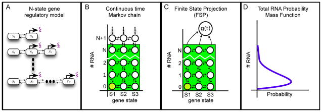
Formulating and solving discrete stochastic models to capture single-cell transcriptional heterogeneities. (A) Effects of chromatin modifications or transcription factor binding/unbinding are described using multiple gene states, each with it own characteristic rate of RNA transcription. Adding more gene states in the model can account for increasingly complex biological behaviors. (B) A lattice describing all possible cellular states for a three state model, as determined by the gene state (x-axis, changes by horizontal arrows) and the number of RNA (y-axis, changes by vertical arrows). In general, the RNA number can exceed any finite bound. Thus, the lattice an infinite number of states and the Chemical Master Equation is infinite in dimension. (C) To overcome this infinite dimensionality, the FSP approach truncated the lattice at N RNA. Reaction that leave the truncated states are absorbed into an absorbing state, whose probability is defined as g(t). (D) The resulting finite, linear system can be used to estimate the probabilities of each state in the Markov chain at any finite time. Projecting the FSP solution onto the RNA axis produces the distribution of RNA at each time point.

To analyze the dynamics of different gene activity states and the resulting fluctuations in transcriptional responses, we use the formalism of the chemical master equation (CME, [45]), which we solve using the Finite State Projection approach [40]. This analysis starts by describing the stochastically transitioning gene-states and subsequent transcript or protein production and degradation reactions using a continuous time Markov chain consisting of an infinite number of discrete cellular states. For example, Figure 2B illustrates a Markov chain that describes switching between three possible gene states (horizontal direction) as well as RNA transcription and degradation events (vertical direction). According to this description, each cellular state is an integer vector, x_i = [g_i, m_i], defined by the specific gene state, g_i, and the number of RNA transcripts, m_i. Reactions correspond to jumps from one cellular state to another, x_i → x_j = x_i + s_μ, where the stoichiometry vector, s_μ, defines the effect that the μ^th reaction has on the cellular state. For example, if a transcription or degradation reaction occurs, the number of RNA increases or decreases by one, yet the gene state remains unchanged: s₁ = [0, 1] for production, and s₂ = [0, −1] for degradation. Similarly, if a gene-state transition reaction occurs (horizontal arrows in Figure 2B), the RNA level remains the same, but the gene-state will change: s₃ = [1, 0], and s₄ = [−1, 0]. In the work described below, gene state transitions are to nearest neighbors only, but longer range transitions are easily captured using the same analytical framework. In addition to the reaction directions, one must define the propensity functions, w_μ(x_i)dt, which describe the probability that each μ^th reaction will occur during the next infinitesimal time step of length dt, given the current state x_i. We denote transcription rates from a single copy of the gene in the g^th gene state as w₁(x_i) = k_rgi for each g_i. Degradation is a first order process with rate γ multiplied by the number of molecules available to degrade, w₂(x_i) = γm_i. Finally, transitions from g_i → g_i + 1 or g_i → g_i −1 are defined by the reaction rates, w₃(x) = k_gi,gi+1 and w₄(x) = k_gi, _gi−1 for each g_i.

By describing the lattice of possible gene states and RNA counts as a Markov chain, we can write the probability of being in the $g_i^{\text{th}}$ gene state and containing m_i RNA as P_i(t) = P(x_i, t) = P_gi,mi(i)(t). Each reaction represents a path by which probability can flow out of or into any particular cellular state, x_i, and these collectively define the set of equations known as the chemical master equation [45]:

$$\frac{d}{dt}P({\mathbf{x}}_i,t)=-\sum _{\mu =1}^M{w}_k({\mathbf{x}}_i)P_i({\mathbf{x}}_i,t)+\sum _{\mu =1}^M{w}_{\mu }({\mathbf{x}}_i-{\mathbf{s}}_{\mu })P({\mathbf{x}}_i-{\mathbf{s}}_{\mu },t).$$ (1)

The probability mass functions for all possible states can be collected into vector form as:

$$\mathbf{P}(t)=\left[\begin{array}{ccc}{{\mathbf{P}}_{\mathbf{0}}}^{\mathbf{T}}& {{\mathbf{P}}_{\mathbf{1}}}^{\mathbf{T}}& \dots \end{array}\right]={\left[\left[\begin{array}{cccc}{P}_{1,0}& P_{2,0}& \dots & P_{N_g,0}\end{array}\right]\left[\begin{array}{cccc}{P}_{1,1}& P_{2,1}& \dots & P_{N_g,1}\end{array}\right]\dots \right]}^{\mathbf{T}},$$ (2)

which allows one to write the CME in a simplified matrix form as

$$\frac{d}{dt}\mathbf{P}(t)=\mathbf{AP}(t).$$ (3)

In this expression, the infinitesimal generator, A, has elements:

$$A_{ji}=\{\begin{array}{ll}-{\sum }_{\mu =1}^M{w}_{\mu }({\mathbf{x}}_{\mathbf{i}})\hfill & \text{if}i=j\hfill \\ w_{\mu }({\mathbf{x}}_{\mathbf{i}})\hfill & \text{for}\text{every}j\text{such}\text{that}{\mathbf{x}}_{\mathbf{j}}={\mathbf{x}}_i+{\mathbf{s}}_{\mu }\hfill \\ 0\hfill & \text{elsewhere}\hfill \end{array}.$$ (4)

For the example illustrated in Figure 2B, full CME can be written as:

$$\frac{d}{dt}\left[\begin{array}{c}{\mathbf{P}}_{\mathbf{0}}\\ {\mathbf{P}}_{\mathbf{1}}\\ {\mathbf{P}}_{\mathbf{2}}\\ ⋮\end{array}\right]=\left[\begin{array}{cccc}\mathbf{H}-\mathbf{T}& \mathbf{D}& \mathbf{0}& \dots \\ \mathbf{T}& \mathbf{H}-\mathbf{T}-\mathbf{D}& \mathbf{2}\mathbf{D}& \ddots \\ \mathbf{0}& \mathbf{T}& \mathbf{H}-\mathbf{T}-\mathbf{2}\mathbf{D}& \ddots \\ ⋮& \ddots & \ddots & \ddots \end{array}\right]\left[\begin{array}{c}{\mathbf{P}}_{\mathbf{0}}\\ {\mathbf{P}}_{\mathbf{1}}\\ {\mathbf{P}}_{\mathbf{2}}\\ ⋮\end{array}\right],$$ (5)

where H, T and D denote the contributions to the infinitesimal generator for the gene state transitions, transcription events, and degradation events, respectively. For the three-gene state problem, these matrices are explicitly written as:

$$\mathbf{H}(t)=\left[\begin{array}{ccc}-k_{12}(t)& k_{21}(t)& 0\\ k_{12}(t)& -k_{21}(t)-k_{23}(t)& k_{32}(t)\\ 0& k_{23}(t)& -k_{32}(t)\end{array}\right];\mathbf{T}=\left[\begin{array}{ccc}{k}_{r1}& 0& 0\\ 0& k_{r2}& 0\\ 0& 0& k_{r3}\end{array}\right];\mathbf{D}=\left[\begin{array}{ccc}\delta & 0& 0\\ 0& \delta & 0\\ 0& 0& \delta \end{array}\right].$$ (6)

Similar notation has also been used to describe multi-state gene regulation in several other studies [40, 44, 46].

The CME is often infinite dimensional due to the potential for certain chemical species to reach any countable integer number. For this reason, the CME can only be solved exactly for a few special cases. However, for most gene regulatory processes, one can use stochastic simulations to generate unbiased sample trajectories for the process [36]. Unfortunately, to compare such analyses to data requires very large numbers of simulations. For certain processes, including those described in Figure 2A, one can develop exact simplified analyses to compute the evolution of statistical moments (i.e., means, variances and co-variances) over time. Such approaches are ideal when a large amount of data is available (e.g., when data results from flow cytometry analyses), such that one can obtain precise measurement of the means, variances and higher moments of the probability distributions [12, 32, 26]. However, when data is limited to a few hundred or thousand cells per sample, as is often the case in smRNA-FISH imaging experiments [9, 23, 24, 25, 27], measurement of these statistical moments may be imprecise due to the influence of long distribution tails. For such situations, solving for the full probability distributions is especially valuable. In the next section, we turn to the finite state projection approach (FSP), which allows us to obtain direct and efficient solutions to the CME, at least for the class of gene regulatory processes described above.

3.2. The finite state projection algorithm

The finite state projection approach (FSP, [40]) provides an approximation to the solution of the CME. Rather than try to analyze the infinite set of all states, we instead select a finite subset of states that retains most of the probability for a pre-specified finite time interval. In particular for the bursting gene expression models of the form described in Figure 2, we include all of the states where the number of RNA is less than some integer N_m. The rest of the states are reduced into a single absorbing state. The result is a reduced master equation of the form

$$\frac{d}{dt}\left[\begin{array}{c}{\mathbf{P}}_{\le N_m}^{\mathit{FSP}}(t)\\ \mathbf{g}(t)\end{array}\right]=\left[\begin{array}{cc}{\mathbf{A}}_{\le N_m}& \mathbf{0}\\ -{\mathbf{1}}^T{\mathbf{A}}_{\le N_m}& 0\end{array}\right]\left[\begin{array}{c}{\mathbf{P}}_{\le N_m}^{\mathit{FSP}}(t)\\ \mathbf{g}(t)\end{array}\right].$$ (7)

Or, in terms of the transition, transcription and degradation reactions, the truncated analysis becomes

$$\frac{d}{dt}\left[\begin{array}{c}{\mathbf{P}}_{\mathbf{0}}\\ {\mathbf{P}}_{\mathbf{1}}\\ {\mathbf{P}}_{\mathbf{2}}\\ ⋮\\ {\mathbf{P}}_N\\ g(t)\end{array}\right]=\left[\begin{array}{ccccc}\mathbf{H}-\mathbf{T}& \mathbf{D}& \mathbf{0}& \dots & \mathbf{0}\\ \mathbf{T}& \mathbf{H}-\mathbf{T}-\mathbf{D}& \mathbf{2}\mathbf{D}& \ddots & \mathbf{0}\\ ⋮& \ddots & \ddots & \ddots & ⋮\\ \mathbf{0}& \mathbf{0}& \mathbf{T}& \mathbf{H}-\mathbf{T}-{\mathbf{N}}_{\mathbf{m}}\mathbf{D}& \mathbf{0}\\ \mathbf{0}& \mathbf{0}& \mathbf{0}& {\mathbf{1}}^{\mathbf{T}}\mathbf{T}& \mathbf{0}\end{array}\right]\left[\begin{array}{c}{\mathbf{P}}_{\mathbf{0}}\\ {\mathbf{P}}_{\mathbf{1}}\\ {\mathbf{P}}_{\mathbf{2}}\\ ⋮\\ {\mathbf{P}}_{\mathbf{N}}\\ g(t)\end{array}\right].$$ (8)

The FSP solution, $P_{\le N_m}^{\mathit{FSP}}(t)$, is an approximate solution to the CME and g(t) is the computable error in the approximation. The FSP theorems guarantee that the FSP is a lower bound on the true solution ${\mathbf{P}}_{\le N_m}^{\mathit{FSP}}\le {\mathbf{P}}_{\le N_m}$, and the total error in the approximation is

$$\left|\left[\begin{array}{c}{\mathbf{P}}_{\le N_m}\\ {\mathbf{P}}_{>N_m}\end{array}\right]-\left[\begin{array}{c}{\mathbf{P}}_{\le N_m}^{\mathit{FSP}}\\ 0\end{array}\right]\right|=g(t).$$ (9)

We note than the original description of the FSP [40], showed only that $\mid {\mathbf{P}}_{\le N_m}-{\mathbf{P}}_{\le N_m}^{\mathit{FSP}}\mid \le g(t)$. For a simple proof of the stronger result in Eq. (9), we refer the interested reader to Ref. [47].

In practice, the matrix in Eq. (8) can be extended until the solution is within some error tolerance (g(t) < ε). However, when typical maximum numbers of RNA are known from experimental observations, this truncation can be applied directly. The matrix in Eq. (8) is a finite set of linear of ordinary differential equations, which can be solved numerically. For systems where the reaction rates in A are not explicitly dependent on time, this can be solved using matrix exponentiation [40] or using Krylov subspace methods [48]. For systems with explicit time dependence, one can solve the truncated master equation using more general linear ODE solvers. We note that the infinitesimal generator in the CME is sparse and often numerically stiff, and its solution is much more tractable using implicit ODE solvers that make use of system sparsity. For the analyses discussed below, we have conducted this integration using Mathworks Matlab’s built-in exponentiation routine “expm” or the stiff ODE integration algorithm “ode15s.”

3.3. Analysis of mRNA accumulation at transcriptional sites

The FSP approach can also be used to compute the probability distribution for the number of nascent transcripts at transcription sites [27]. For a model with n gene states, the probability distribution for the gene states evolves according to the simple n-dimensional ODE given by:

$$\frac{d}{dt}{\mathbf{P}}_{\text{gene}}=\mathbf{H}(t){\mathbf{P}}_{\text{gene}},$$ (10)

where H(t) is as defined above in Eq. (6). Each of the n different gene states has its own characteristic transcription initiation rate. We now assume that the transcription process takes less than a fixed finite amount of time, τ to complete. Under this assumption, the number of nascent transcripts at time t is exactly the number of transcripts that have initiated transcription, but have not yet completed (or been interrupted) in the time interval from t − τ to t. Since all RNA initiated prior to or at time t − τ are no longer at the transcription site, their actual number at that time is irrelevant to the number at time t. For simplicity in computation, we can assume that there are no nascent RNA at time t − τ. As a result, solving for the number of nascent RNA at time t_i becomes equivalent to solving Eq. (8), with an initial probability distribution specified as: P₀(t_i − τ) = P_gene(t_i − τ) and P_m(t_i − τ) = 0 for m ≥ 1. If one assumes that RNA cannot degrade or otherwise be disrupted during their elongation process [27], then the degradation matrix D in Eq. (8) should be adjusted accordingly.

3.4. Computing and maximizing the likelihood of smRNA-FISH data

smRNA-FISH data is collected by counting fluorescently tagged RNA of interest in many single cells as discussed in Section 2. By counting the RNA in each of a set of C fixed cells at a given time t, one can quantify a probability distribution for the number of observed RNA at that time. With a model parameterized by θ that can generate a probability distribution of observing a cell with m RNA under that specific condition and time, one can compute the logarithm of the likelihood of the data as:

$$logL(\mathbf{D}\mid \theta )=\sum _{c=1}^{C}logp(m_c\mid \theta ),$$ (11)

where m_c is the number of mRNA in the c^th cell. Equivalently, this sum can be rewritten as

$$logL(\mathbf{D}\mid \theta )=\sum _{i=0}^M{q}_{i}logp(i\mid \theta ),$$ (12)

where q_i is the number of cells with exactly i RNA, M is the maximum number of RNA experimentally observed in a single cell, and θ is a vector of model parameters.

A good model choice of model parameters, θ_fit, should be expected to maximize this log-likelihood,

$${\theta }_{\mathit{fit}}=\underset{\theta }{\text{argmax}}\sum _{i=0}^M{q}_{i}logp(i\mid \theta ).$$ (13)

We note that the parameter value that minimizes Eq. (13) is the same as the minimum of the Kullback-Leibler divergence between the experimentally measured distribution q_i/Σq_i and the model distributions, and the model distribution, p(i):

$$\mathit{KLD}\left(\frac{q(i)}{Q},p(i)\right)=\sum _{i=0}^M\frac{q_i}{Q}\left(log(p(i\mid \theta ))-log\left(\frac{q_i}{Q}\right)\right),$$ (14)

However, in the case of multiple time points, the log-likelihoods are summed over each time. When this value is constant over time (i.e., when all cell populations have equal sizes) both the KLD and maximum likelihood yield the same parameter values. To maximize the likelihood function, we use a hybridization of local and global optimization schemes. For local searches, we utilize the simplex search method implemented in the built-in Matlab routine, ‘fminsearch’. For global searches, we use Matlab’s built-in genetic algorithm search method, ‘ga’. In practice, these global and local algorithms are iterated and run many times from different initial parameter guesses.

We note that other approaches approximate likelihoods through comparisons of summary statistics, such as means and variances [32, 49]. Although current implementations of the FSP approach are limited to simpler models, direct comparison of distributions is highly beneficial when restricted to a finite number of cells, such as is the case for mRNA-FISH investigations. In these circumstances, it may be difficult to measure or estimate the uncertainties in more than the first one or two moments, whereas comparison of full distributions remains a straightforward task, even when the moments are not well estimated.

4. Example Studies

To illustrate the combined use of smRNA-FISH analyses and finite state projection analyses, we next show how these tools have been applied to measure and model the single-cell distributions of RNA in bacteria, yeast and human cells. For these different systems, we examine different types of RNA: small non-coding RNA (sRNA) in bacteria, nascent mRNA at transcription sites in human-derived cells, and fully mature mRNA in yeast cells. These RNA have been measured using the three different smRNA-FISH approaches described above in Figure 1B–D, and for each we identify different n-state regulatory models. Although the specifics are different from one case to the next, in all cases the smRNA-FISH data can be captured and in some cases predicted with strong quantitative accuracy using the FSP approach.

4.1. smFISH and FSP in bacteria

We begin by looking at recent measurements of small RNA in bacteria made in reference [22]. Because sRNA are much shorter than most mRNA molecules to which smRNA-FISH has been applied, the authors of this work developed quencher probes that silenced the fluorescence of non-specifically bound probes (see Figure 1D). This allowed them to get accurate measurements of the number of sRNA at the level of individual cells (see Figure 1D for a representative image). The authors specifically explored two different sRNA in two different bacteria: Yersinia-specific sRNA-35 (YSR35), which is a 339-nucleotide long sRNA in Y. pseudotuberculosis and YSP8, which is a 312-nucleotide long sRNA in Y. pestis. These sRNA were labeled with 15 (YSR35) or 12 (YSP8) probes per sRNA as described in reference [22]. Both of these two sRNA were previously known to be up-regulated due to a shift from room temperature (25°C) to human body temperature (37°C). To get sufficient statistics of the system’s regulatory response, measurements were taken in approximately 10,000 bacteria per experimental condition. In both cases, the majority of cells expressed no sRNA, and the distributions of sRNA per cell appeared to be strongly similar to a geometric distribution (see Figure 3B, blue bars).

A two-state model (see Figure 3A) was proposed to match the regulated distributions of sRNA for the system. The authors explored two different possibilities for this model: one where temperature changed with the rate of activation (k₁₂) and one where temperature regulation changed the rate of deactivation (k₂₁). For each model, the FSP implementation was defined as given in Eqs. (6) and (8), where either k₁₂ or k₂₁ was assumed to be condition dependent. Parameter estimation was carried out as described above, and all parameters were fit to reproduce the measured distributions. It was determined that the model where k₁₂ fluctuated from one condition to the next provided the best reproduction of the measured results. Figure 3B shows the resulting two-state k₁₂-modulated model fit to the distributions of YSP8 in Y. Pestis at the initial steady state of 25°C as well as at two and three hours post transition to 37°C. Similar analysis was also applied to measurement of the YSR35 in Y. pseudotuberculosis, for which the same mechanism (k₁₂-modulated regulation) also fit best to the measured distributions (see Reference [22], Figure 5). Using the FSP algorithm, solving for the YSR8 transcript distributions takes an average of 0.0015 seconds to complete per parameter combination (on a 2.6 GHz Intel Core i7 Macbook Pro using Matlab’s built in matrix exponentiation command “expm”).

Parameters for these results are shown in Table 1. In this case, there is insufficient temporal data to fully constrain all parameter values, such that the identified parameter set is not unique. To reduce the dimensionality of the parameter space, the degradation rate was assumed to be 1 min⁻¹. Furthermore, it was found that k₂₁ and the transcript production rates, k_r2 were large compared to the degradation and activation rates, such that k₂₁ and k_r2 could not be determined separately. However, the ratio of these two variable defines an identifiable average burst size μ_burst = k_r2/k₂₁. Although this analysis sufficed to reveal the general mechanism of temperature-sensitive frequency modulation of sRNA expression, additional experimental evidence would be necessary to fully identify the parameters of the dynamical system. In particular, since the RNA dynamics occur on a time scale of a few minutes, it would be necessary to quantify biological responses along the same or similar time scale. To illustrate the importance of dynamics, the next two examples examine mRNA regulation in eukaryotes with more complicated input functions and at faster time scales.

Table 1.

Parameters found to fit a two-state k₁₂-modulated model of YSP8 sRNA transcription activation in Y. pestis bacteria following temperature elevation.

Parameter Name	Value	Units
kr2/k21	1.19	molecules
γ	1.00	min−1
k12 at 25°C	0.138	min−1
k12 at 37°C, 2hr	0.161	min−1
k12 at 37°C, 3hr	0.286	min−1

4.2. smFISH and FSP in human cells

A second study in which single-cell measurements were integrated with discrete stochastic analyses and the FSP approach was examined in Reference [27]. In this case, the authors explored the effects that spatiotemporal dynamics of the ERK1/2 kinase signal had on the activation of c-Fos transcription in human derived osteosarcoma cells (U2OS). Upon induction via the addition of fetal calf serum, the ERK1/2 kinase is phosphorylated to its active form, and immunofluorescence staining was used to quantify the nuclear translocation of the phosphorylated kinase (p-ERK) over time in individual cells. As shown in Figure 4A, this provided a quantitative measurement of the time-varying input component, which could then affect the rates of transitions between different gene states as illustrated in Figure 4B. The downstream activation of c-Fos mRNA was then quantified using single molecule fluorescence in situ hybridization using multiple-label smRNA-FISH probes (see Figure 1B for a representative image). These experimental measurements can only observe and distinguish an active transcription site (TS) from a mature mRNA if it has more two or more nascent mRNA. As such, active TS’s are defined in the model as those that contain at least two mRNA, and as a result an active TS could correspond to any actual gene state. In this case, the authors quantified the probability that a TS would be active (see Figure 4C), the number of nascent mRNA per active TS (see Figure 4D), and the total number of mature mRNA in each cell. Using these experiments, it was observed that non-induced cells contained no detectable active transcription sites and expressed an average of only 4 mature mRNA per cell. After 30 min of serum induction, cells contained an average of 90 mature mRNA with a large variability (some have only a few mRNA, while others contain hundreds). The number of active transcript sites (TS’s) and mature mRNA had correlated temporal dynamics, but the distribution of nascent mRNA on activated alleles was found to be largely independent of condition [27].

Figure 4.

Experimental and computational analyses of cFos transcription in human U20S cells. Experimental data are shown in blue and model results are illustrated in red. Figure is adapted from reference [27]. A) Immunofluorescence measurements of phosphorylated ERK kinase versus time following serum induction, in terms of normalized units. Magenta and cyan horizontal lines correspond to the p-ERK thresholds at which the k₁₂ and k₂₃ reaction rates become greater than zero (see Table 2). B) Model for the induction of c-Fos in response to p-ERK signaling. In the absence of p-ERK, all cells begin in the ‘OFF’ state. Addition of moderate p-ERK levels quickly leads to a primary activation state, ‘on’. When p-ERK levels are very high, a secondary activation state, ‘ON,’ is reached. C) Probability that a given transcription site will be active as a function of time following serum induction. D) Probability distributions of the number of nascent RNA per transcription site at different times following serum induction. Rates for all reactions and the dependency on p-ERK signal are given in Table 2.

The authors then examined different bursting gene expression models of the form illustrated in Figure 2A to determine if these could capture the measured distributions of active transcription sites, nascent mRNA levels and mature mRNA levels [27]. In this case, it was found that a 2-state model could capture most of the full distributions of nascent mRNA at individual transcription sites. However, at maximal activation, which occurred twenty minutes following activation, the data revealed an additional transcriptional mode, which could not be explained with the 2-state model. This high-activity mode, which is well captured by the 3-state model (see Figure 4B), leads to a temporary increase in the number of nascent mRNA per TS in the more activated cells (see 20 minute time point in Figure 4D). In order to reproduce the probabilities of transcription site activation and the distributions for the number of nascent mRNA per transcription site, the parameters were identified as given in Table 2.

Table 2.

Parameters found to fit a three-state model to the activation of transcription sites and the probability distributions for mRNA per transcription sites. The p-ERK input signal denoted as u(t) in the expressions for k₁₂(t) and k₂₃(t) is interpolated from the curve shown in Figure 4 and normalized to have a peak magnitude of one (arbitrary units).

Parameter Name	Value	Units
k12	max(0, −0.102 + 0.198 · u(t))	min−1
k21	0.329	min−1
k23	max(0, −12.7 + 12.9 · u(t))	min−1
k32	0.150	min−1
kr2	34.4	molecules/min
kr3	70.126	molecules/min
τ	0.126	min

Parameters in the final identified 3-state model were such that the rates of transcript elongation were fast relative to the amount of time a given cell would spend in active transcriptional states (k₂₁ and k₃₂ ≪ τ⁻¹). These parameters lead to an effective saturation of bursts at the transcription sites, which explains why the nascent mRNA distributions are uncorrelated with the number of transcription sites or the mature mRNA levels in most conditions [27]. Applying the modified FSP algorithm, setting up the analysis and solving for the nascent c-Fos transcript distributions at all time points takes approximately 0.17 seconds to complete per parameter combination (on a 2.6 GHz Intel Core i7 Macbook Pro using Matlab’s built in ODE integrator “ode15s”).

4.3. smFISH and FSP in yeast cells

In Reference [9], the authors used smRNA-FISH and FSP analyses to quantify dynamic distributions of several mRNA in Saccharomyces cerevisiae cells in response to osmotic shock. Exposure to a high salt environment activates the well characterized high-osmolarity glycerol (HOG) MAPK pathway in yeast [50]. Upon phosphorylation, the kinase signaling molecule, Hog1-p rapidly migrates to the nucleus [9, 51]. To quantify this translocation, Hog1 was fused to yellow fluorescent protein, and the migration of construct Hog1p-YFP into the nucleus was experimentally measured using fluorescence time lapse microscopy. Figure 5A shows the resulting quantification of this time-varying input signal at step inputs of 0.4M and 0.2M NaCl [9]. Once in the nucleus, Hog1-p activates mRNA expression for several genes, including STL1, CTT1, and HSP12. The authors designed smRNA-FISH probes to quantify expression of the different mRNA, and Figure 5C shows representative examples of the resulting distributions over time. Unlike the nuclear enrichment signal which shows little cell-to-cell variability, the transcript expression varies considerably from cell to cell.

The authors then proposed a large class of models, including two-, three-, four- and five-state models with different mechanisms by which Hog1-p could affect transitions between gene states [9]. Each model was then fit to maximize the likelihood of the experimental data using the FSP approach outlined above. In this case, solving for the mRNA distributions at all time points takes under 0.4 seconds to complete per parameter combination (on a 2.6 GHz Intel Core i7 Macbook Pro using Matlab’s built in ODE integration routine “ode15s”). As expected, model fits improve with increased complexity, but this could also lead to overfitting and a loss of predictive power. To analyze the level of overfitting for a particular model, each model was cross-validated using different independent experimental replicas. After a certain level of model complexity, the fits continue to improve, but cross-validation shows that parameter uncertainty also increases, and predictions are expected to worsen. This suggests a “Goldilock’s model,” which is neither too complex nor too simple, that yields optimally accurate predictions. In this case, this optimal model consists of four gene states, where the stochastic transitions from the second state to the first state (i.e., reaction rate k₂₁) is repressed by the time-varying Hog1-p signal as shown in Figure 5B.

This model structure (shown in Figure 5B) and parameters (provided in Table 3) suggest the mechanisms by which STL1 and CTT1 gene expression are controlled by Hog1-p in response to osmotic shock. In the absence of Hog1-p, cells are primarily in the ‘OFF’ state, but occasionally sample the S2 state. While Hog1-p is below the cyan line in Figure 5A, the S2 state is highly unstable, and most cells quickly transition back to the OFF state without significant mRNA accumulation. Addition of Hog1-p near to or above this value stabilizes the S2 state and allows cells to continue to the fully active S3 and S4 states. Although both STL1 and CTT1 have the same activation dynamics, their deactivation processes are slight different. In particular, the rates leading to deactivation (k₃₂, k₄₃ and γ) are all much lower for CTT1 than for STL1. To investigate the generality of the chosen four-state model, the authors used established S. cerevisiae strains with chromatin modifiers Arp8p or Gcn5p knockouts, or with a five-fold over-expression of the transcription factor Hot1p. In each strain, transcript expression dynamics of STL1, CTT1, and HSP12 were observed. The interplay between relatively uniform activation and modulated deactivation rates in the chosen four-state model was sufficient to capture and predict the full, time-varying mRNA distributions for each gene and mutant strain [9].

Table 3.

Parameters found to fit a four-state k₂₁-modulated model of Hog1-p induced transcription of STL1 and CTT1 mRNA transcription activation in S. cerevisiae following application of osmotic shock (adapted from reference [9], Table S2). The Hog1-p input signal (see Figure 5A) is denoted as u(t) in the expressions for k₂₁(t).

Parameter Name	STL1	CTT1	Units
k12	1.29	1.29	s−1
k21	max(0, 3200 − 7710 · u(t))	max(0, 3200 − 7710 · u(t))	s−1
k23	0.0067	0.0191	s−1
k32	0.027	0.0175	s−1
k34	0.133	0.133	s−1
k43	0.0381	0.0083	s−1
kr2	0.0116	0.0098	molecules/s
kr3	0.987	1.01	molecules/s
kr4	0.0538	0.0016	molecules/s
γ	0.0049	0.0020	s−1

5. Conclusions

In this article, we reviewed current experimental approaches to study biological noise in gene expression such as time-lapse fluorescence microscopy and Single-Molecule RNA fluorescence In Situ Hybridization (smRNA-FISH) and flow cytometry. We explored how these techniques could allow for quantification of gene regulatory responses. In particular, we focussed on smRNA-FISH measurements of RNA in fixed biological samples, which provides a direct and fast readout for how transcriptional responses change from cell to cell or over time as a population adapts to fluctuations in the surrounding environment. These experimental techniques are essential to quantify biological noise in RNA and protein expression at the individual cell level, and they have been applied to probe transcriptional regulation dynamics in organisms ranging from bacteria and yeast to human cells. We also discussed current theoretical approaches to integrate dynamic single-cell data sets with discrete stochastic computational analyses. Here, our focus has been to identify model parameters given experimentally measured distributions of RNA at the single-molecule and single-cell levels, especially during transient environmental changes. Although numerous theoretical techniques, including moment closure techniques [16, 26, 32, 33, 34, 35, 49] and kinetic Monte Carlo simulations [14, 15], have been used successfully to perform such analyses, we focussed here on the application of Finite State Projection (FSP) approach [40]. The FSP approach provides an precise approximate solution to the Chemical Master Equation with known error [40], which enables direct comparison of models to measured experimental data. For many important signal-activated gene transcriptional processes in bacteria [12, 13, 22], yeast [9] and mammalian cells [27], the FSP approach is ideal because it can solve for the full time-varying single-cell mRNA probability distributions in a fraction of a second.

The goal of our approach to integrate experiments with computational approaches, is to build a cohesive framework that reaches a balance between what is biologically important and what kind of predictive models can be supported with specific data sets. Given the complexity of biological models and the limited number of high quality data sets, this is a challenging task. However, it is a task that has been proven to be resolvable in a small set of studies. Here, we have presented three cases to demonstrate the generality of this approach in bacteria [22], yeast [9] and human cells [27]. The data-centered approach presented here differs from many past mechanistic modeling endeavors in that our goal is to fit and predict all observed biological fluctuations, but our models are not restricted to previously known biophysical mechanisms. As such, the identified models simultaneously capture those fluctuations inherent to the measured RNA species as well as those due to upstream influences. If available, mechanistic understanding based upon prior biochemical understanding can then be used to separate these different aspects of biological fluctuations into intrinsic and extrinsic noise. Although this data-centered approach can provide detailed quantitative predictions for cell population behaviors, its direct insight into the underlying biochemical nature of gene expression variability is more limited. In the future, we expect that such abstract models need to be combined with genetic knockout studies to attach biochemical and mechanistic meaning to specific rates and gene states in the models. If successful, this next step would enable computational models to enable a greater range of biologically meaningful predictions. For example, in Reference [9], we found that linking parameters to different chromatin modifiers and transcription factors enabled the precise quantitative predictions for the responses of novel combinations of genetic mutations and transcriptional outputs. In the long term, such combined experimental and computational approaches are needed to better understand biological networks that must be studied at greater complexities than one gene at a time. Furthermore, applying systematic approaches to identify models that accurately predict gene responses (such as transitions between healthy and diseased phenotypes) in different environments may eventually help guide decisions in future personalized medicine applications.

1. We review experimental tools to quantify single-cell transcription fluctuations.

2. The finite state projection accurately reproduces these single-cell measurements.

3. Integrating computation and experiments helps to understand cellular variation.

4. Cellular heterogeneities or noise reveal hidden gene regulatory mechanisms.

5. We review results for three different RNA types in three different organisms.

References

- 1.Gerdes MJ, Sevinsky CJ, Sood A, Adak S, Bello MO, Bordwell A, Can A, Corwin A, Dinn S, Filkins RJ, Hollman D, Kamath V, Kaanumalle S, Kenny K, Larsen M, Lazare M, Li Q, Lowes C, McCulloch CC, McDonough E, Montalto MC, Pang Z, Rittscher J, Santamaria-Pang A, Sarachan BD, Seel ML, Seppo A, Shaikh K, Sui Y, Zhang J, Ginty F. Highly multiplexed single-cell analysis of formalin-fixed, paraffin-embedded cancer tissue. Proceedings of the National Academy of Sciences of the United States of America. 2013;110(29):11982–11987. doi: 10.1073/pnas.1300136110. [DOI] [PMC free article] [PubMed] [Google Scholar]
- 2.Krutzik PO, Nolan GP. Fluorescent cell barcoding in flow cytometry allows high-throughput drug screening and signaling profiling. Nature Methods. 2006;3(5):361–368. doi: 10.1038/nmeth872. [DOI] [PubMed] [Google Scholar]
- 3.Shapiro E, Biezuner T, Linnarsson S. Single-cell sequencing-based technologies will revolutionize whole-organism science. Nature Reviews Genetics. 2013;14(9):618–630. doi: 10.1038/nrg3542. [DOI] [PubMed] [Google Scholar]
- 4.Gahlmann A, Moerner WE. Exploring bacterial cell biology with single-molecule tracking and super-resolution imaging. Nature Reviews Microbiology. 2014;12(1):9–22. doi: 10.1038/nrmicro3154. [DOI] [PMC free article] [PubMed] [Google Scholar]
- 5.Klipp E, Nordlander B, Krüger R, Gennemark P, Hohmann S. Integrative model of the response of yeast to osmotic shock. Nature Biotechnology. 2005;23(8):975–982. doi: 10.1038/nbt1114. [DOI] [PubMed] [Google Scholar]
- 6.Macklin DN, Ruggero NA, Covert MW. The future of whole-cell modeling. Current Opinion in Biotechnology. 2014;28:111–115. doi: 10.1016/j.copbio.2014.01.012. [DOI] [PMC free article] [PubMed] [Google Scholar]
- 7.Mettetal JT, Muzzey D, Gomez-Uribe C, van Oudenaarden A. The Frequency Dependence of Osmo-Adaptation in Saccharomyces cerevisiae. Science. 2008;319(5862):482–484. doi: 10.1126/science.1151582. [DOI] [PMC free article] [PubMed] [Google Scholar]
- 8.Alon U. An Introduction to Systems Biology: Design Principles of Biological Circuits. Chapman and Hall/CRC; 2006. [Google Scholar]
- 9.Neuert G, Munsky B, Tan RZ, Teytelman L, Khammash M, van Oudenaarden A. Systematic identification of signal-activated stochastic gene regulation. Science. 2013;339(6119):584–587. doi: 10.1126/science.1231456. [DOI] [PMC free article] [PubMed] [Google Scholar]
- 10.Gutenkunst RN, Waterfall JJ, Casey FP, Brown KS, Myers CR, Sethna JP. Universally sloppy parameter sensitivities in systems biology models. PLoS Computational Biology. 2007;3(10):1871–1878. doi: 10.1371/journal.pcbi.0030189. [DOI] [PMC free article] [PubMed] [Google Scholar]
- 11.Villaverde AF, Banga JR. Reverse engineering and identification in systems biology: strategies, perspectives and challenges, Journal of the Royal Society. Interface / the Royal Society. 2014;11(91):20130505–20130505. doi: 10.1098/rsif.2013.0505. [DOI] [PMC free article] [PubMed] [Google Scholar]
- 12.Munsky B, Trinh B, Khammash M. Listening to the noise: random fluctuations reveal gene network parameters. Molecular Systems Biology. 2009;5:318. doi: 10.1038/msb.2009.75. [DOI] [PMC free article] [PubMed] [Google Scholar]
- 13.Lou C, Stanton B, Chen YJ, Munsky B, Voigt CA. Ribozyme-based insulator parts buffer synthetic circuits from genetic context. Nature Biotechnology. 2012;30(11):1137–1142. doi: 10.1038/nbt.2401. [DOI] [PMC free article] [PubMed] [Google Scholar]
- 14.Viñuelas J, Kaneko G, Coulon A, Vallin E, Morin V, Mejia-Pous C, Kupiec JJ, Beslon G, Gandrillon O. Quantifying the contribution of chromatin dynamics to stochastic gene expression reveals long, locus-dependent periods between transcriptional bursts. BMC Biology. 2013;11(1):15. doi: 10.1186/1741-7007-11-15. [DOI] [PMC free article] [PubMed] [Google Scholar]
- 15.Lillacci G, Khammash M. The signal within the noise: efficient inference of stochastic gene regulation models using fluorescence histograms and stochastic simulations. Bioinformatics. 2013;29(18):2311–2319. doi: 10.1093/bioinformatics/btt380. [DOI] [PubMed] [Google Scholar]
- 16.Lipinski-Kruszka J, Stewart-Ornstein J, Chevalier MW, El-Samad H. Using Dynamic Noise Propagation to Infer Causal Regulatory Relationships in Biochemical Networks. ACS Synthetic Biology. 2015;4(3):258–264. doi: 10.1021/sb5000059. [DOI] [PMC free article] [PubMed] [Google Scholar]
- 17.Molina N, Suter DM, Cannavo R, Zoller B, Gotic I, Naef F. Stimulus-induced modulation of transcriptional bursting in a single mammalian gene. Proceedings of the National Academy of Sciences of the United States of America. 2013;110(51):20563–20568. doi: 10.1073/pnas.1312310110. [DOI] [PMC free article] [PubMed] [Google Scholar]
- 18.Harper CV, Finkenstädt B, Woodcock DJ, Friedrichsen S, Semprini S, Ashall L, Spiller DG, Mullins JJ, Rand DA, Davis JRE, White MRH. Dynamic analysis of stochastic transcription cycles. PLoS Biology. 2011;9(4):e1000607. doi: 10.1371/journal.pbio.1000607. [DOI] [PMC free article] [PubMed] [Google Scholar]
- 19.Zechner C, Unger M, Pelet S, Peter M, Koeppl H. Scalable inference of heterogeneous reaction kinetics from pooled single-cell recordings. Nature Methods. 2014;11(2):197–202. doi: 10.1038/nmeth.2794. [DOI] [PubMed] [Google Scholar]
- 20.Bothma JP, Garcia HG, Esposito E, Schlissel G, Gregor T, Levine M. Dynamic regulation of eve stripe 2 expression reveals transcriptional bursts in living Drosophila embryos. Proceedings of the National Academy of Sciences of the United States of America. 2014;111(29):10598–10603. doi: 10.1073/pnas.1410022111. [DOI] [PMC free article] [PubMed] [Google Scholar]
- 21.Kiviet DJ, Nghe P, Walker N, Boulineau S, Sunderlikova V, Tans SJ. Stochasticity of metabolism and growth at the single-cell level. Nature. 2014;514(7522):376–379. doi: 10.1038/nature13582. [DOI] [PubMed] [Google Scholar]
- 22.Shepherd DP, Li N, Micheva-Viteva SN, Munsky B, Hong-Geller E, Werner JH. Counting small RNA in pathogenic bacteria. Analytical Chemistry. 2013;85(10):4938–4943. doi: 10.1021/ac303792p. [DOI] [PubMed] [Google Scholar]
- 23.Zenklusen D, Larson DR, Singer RH. Single-RNA counting reveals alternative modes of gene expression in yeast. Nature Structural and Molecular Biology. 2008;15(12):1263–1271. doi: 10.1038/nsmb.1514. [DOI] [PMC free article] [PubMed] [Google Scholar]
- 24.Tan RZ, van Oudenaarden A. Transcript counting in single cells reveals dynamics of rDNA transcription. Molecular Systems Biology. 2010;6(1):358. doi: 10.1038/msb.2010.14. [DOI] [PMC free article] [PubMed] [Google Scholar]
- 25.Bumgarner SL, Neuert G, Voight BF, Symbor-Nagrabska A, Grisafi P, van Oudenaarden A, Fink GR. Single-cell analysis reveals that noncoding RNAs contribute to clonal heterogeneity by modulating transcription factor recruitment. Molecular Cell. 2012;45(4):470–482. doi: 10.1016/j.molcel.2011.11.029. [DOI] [PMC free article] [PubMed] [Google Scholar]
- 26.Singh A, Razooky BS, Dar RD, Weinberger LS. Dynamics of protein noise can distinguish between alternate sources of gene-expression variability. Molecular Systems Biology. 2012;8(1):607. doi: 10.1038/msb.2012.38. [DOI] [PMC free article] [PubMed] [Google Scholar]
- 27.Senecal A, Munsky B, Proux F, Ly N, Braye FE, Zimmer C, Mueller F, Darzacq X. Transcription factors modulate c-Fos transcriptional bursts. Cell Reports. 2014;8(1):75–83. doi: 10.1016/j.celrep.2014.05.053. [DOI] [PMC free article] [PubMed] [Google Scholar]
- 28.Kim JK, Marioni JC. Inferring the kinetics of stochastic gene expression from single-cell RNA-sequencing data. Genome Biology. 2013;14(1):R7. doi: 10.1186/gb-2013-14-1-r7. [DOI] [PMC free article] [PubMed] [Google Scholar]
- 29.Bajikar SS, Fuchs C, Roller A, Theis FJ, Janes KA. Parameterizing cell-to-cell regulatory heterogeneities via stochastic transcriptional profiles. Proceedings of the National Academy of Sciences of the United States of America. 2014;111(5):E626–35. doi: 10.1073/pnas.1311647111. [DOI] [PMC free article] [PubMed] [Google Scholar]
- 30.Munsky B, Neuert G, van Oudenaarden A. Using gene expression noise to understand gene regulation. Science. 2012;336(6078):183–187. doi: 10.1126/science.1216379. [DOI] [PMC free article] [PubMed] [Google Scholar]
- 31.Munsky B, Neuert G. From Analog to Digital Models of Gene Regulation. Physical Biology. doi: 10.1088/1478-3975/12/4/045004. in press. [DOI] [PMC free article] [PubMed] [Google Scholar]
- 32.Ruess J, Milias-Argeitis A, Lygeros J. Designing experiments to understand the variability in biochemical reaction networks, Journal of the Royal Society. Interface / the Royal Society. 2013;10(88):20130588–20130588. doi: 10.1098/rsif.2013.0588. [DOI] [PMC free article] [PubMed] [Google Scholar]
- 33.Schwabe A, Bruggeman FJ. Single yeast cells vary in transcription activity not in delay time after a metabolic shift. Nature Communications. 2014;5(1):4798. doi: 10.1038/ncomms5798. [DOI] [PubMed] [Google Scholar]
- 34.So LH, Ghosh A, Zong C, Sepúlveda LA, Segev R, Golding I. General properties of transcriptional time series in Escherichia coli. Nature Genetics. 2011;43(6):554–560. doi: 10.1038/ng.821. [DOI] [PMC free article] [PubMed] [Google Scholar]
- 35.Komorowski M, Costa MJ, Rand DA, Stumpf MPH. Sensitivity, robustness, and identifiability in stochastic chemical kinetics models. Proceedings of the National Academy of Sciences of the United States of America. 2011;108(21):8645–8650. doi: 10.1073/pnas.1015814108. [DOI] [PMC free article] [PubMed] [Google Scholar]
- 36.Gillespie DT. Exact stochastic simulation of coupled chemical reactions. J Physical Chemistry. 1977;81:2340–2361. [Google Scholar]
- 37.Suter DM, Molina N, Gatfield D, Schneider K, Schibler U, Naef F. Mammalian genes are transcribed with widely different bursting kinetics. Science. 2011;332(6028):472–474. doi: 10.1126/science.1198817. [DOI] [PubMed] [Google Scholar]
- 38.Raj A, van den Bogaard P, Rifkin SA, van Oudenaarden A, Tyagi S. Imaging individual mRNA molecules using multiple singly labeled probes. Nature Methods. 2008;5(10):877–879. doi: 10.1038/nmeth.1253. [DOI] [PMC free article] [PubMed] [Google Scholar]
- 39.Femino AM, Fay FS, Fogarty K, Singer RH. Visualization of single RNA transcripts in situ. Science. 1998;280(5363):585–590. doi: 10.1126/science.280.5363.585. [DOI] [PubMed] [Google Scholar]
- 40.Munsky B, Khammash M. The finite state projection algorithm for the solution of the chemical master equation. The Journal of Chemical Physics. 2006;124(4):044104. doi: 10.1063/1.2145882. [DOI] [PubMed] [Google Scholar]
- 41.Dong GQ, McMillen DR. Effects of protein maturation on the noise in gene expression. Physis Review E. 2008;77(2):021908. doi: 10.1103/PhysRevE.77.021908. [DOI] [PubMed] [Google Scholar]
- 42.Femino AM, Fogarty K, Lifshitz LM, Carrington W, Singer RH. Visualization of single molecules of mRNA in situ. Methods in Enzymology. 2003;361:245–304. doi: 10.1016/s0076-6879(03)61015-3. [DOI] [PubMed] [Google Scholar]
- 43.Ko MS. A stochastic model for gene induction. Journal of Theoretical Biology. 1991;153(2):181–194. doi: 10.1016/s0022-5193(05)80421-7. [DOI] [PubMed] [Google Scholar]
- 44.Peccoud J, Ycart B. Markovian modeling of gene-product synthesis. Theoretical Population Biology. 1995;48(2):222–234. [Google Scholar]
- 45.van Kampen N. Stochastic Processes in Physics and Chemistry. 3. Elsevier; 2007. [Google Scholar]
- 46.Sanchez A, Kondev J. Transcriptional Control of Noise in Gene Expression. Proceedings of the National Academy of Sciences of the United States of America. 2008;105(13):5081–5086. doi: 10.1073/pnas.0707904105. [DOI] [PMC free article] [PubMed] [Google Scholar]
- 47.Munsky B. Modeling cellular variability. In: Wall ME, editor. Quantitative Biology From Molecular to Cellular Systems. Taylor & Francis Group; New York, NY: 2012. pp. 233–266. [Google Scholar]
- 48.Burrage K, Hegland M, Macnamara S, Sidje R. A Krylov-Based Finite State Projection Algorithm for Solving the Chemical Master Equation Arising in the Discrete Modelling of Biological Systems. Proceedings of The AA Markov 150th Anniversary Meeting. 2006:21–37. [Google Scholar]
- 49.Zechner C, Ruess J, Krenn P, Pelet S, Peter M, Lygeros J, Koeppl H. Moment-based inference predicts bimodality in transient gene expression. Proceedings of the National Academy of Sciences of the United States of America. 2012;109(21):8340–8345. doi: 10.1073/pnas.1200161109. [DOI] [PMC free article] [PubMed] [Google Scholar]
- 50.Brewster JL, Gustin MC. Hog1: 20 years of discovery and impact. Science Signaling. 2014;7(343):1–10. doi: 10.1126/scisignal.2005458. [DOI] [PubMed] [Google Scholar]
- 51.Muzzey D, Gomez-Uribe CA, Mettetal JT, van Oudenaarden A. A Systems-Level Analysis of Perfect Adaptation in Yeast Osmoregulation. Cell. 2009;138(1):160–171. doi: 10.1016/j.cell.2009.04.047. [DOI] [PMC free article] [PubMed] [Google Scholar]