Surface Laplacians (SL) and phase properties of EEG rhythms: simulated generators in a volume-conduction model

Abstract

Surface Laplacian (SL) methods offer advantages in spectral analysis owing to the well-known implications of volume conduction. Although recognition of the superiority of SL over reference-dependent measures is widespread, well-reasoned cautions have precluded their universal adoption. Notably, the expected selectivity of SL for superficial rather than deep generators has relegated SL to the role of an add-on to conventional analyses, rather than as an independent area of inquiry, despite empirical findings supporting the consistency and replicability of physiological effects of interest. It has also been reasoned that the contrast-enhancing effects of SL necessarily make it insensitive to broadly distributed generators, including those suspected for oscillatory rhythms such as EEG alpha. These concerns are further exacerbated for phase-sensitive measures (e.g., phase-locking, coherence), where key features of physiological generators have yet to be evaluated. While the neuronal generators of empirically-derived EEG measures cannot be precisely known due to the inverse problem, simple dipole generator configurations can be simulated using a 4-sphere head model and linearly combined. We simulated subdural and deep generators and distributed dipole layers using sine and cosine waveforms, quantified at 67-scalp sites corresponding to those used in previous research. Reference-dependent (nose, average, mastoids reference) EEG and corresponding SL topographies were used to probe signal fidelity in the topography of the measured amplitude spectra, phase and coherence of sinusoidal stimuli at and between “active” recording sites. SL consistently outperformed the conventional EEG measures, indicating that continued reluctance by the research community is unfounded.

1. Introduction

Concerns have frequently been expressed about the fidelity of EEG measures for representing phase-relationships between electrodes recorded in a scalp montage (Biggins et al. 1991, 1992; Pascual-Marqui, 1993; Nunez et al., 1997; Qin et al., 2010). This concern is relevant for oscillatory activity, because volume conduction combines nearby rhythms that share a common frequency. The resulting composite waveforms at nearby sites may become indistinguishable, being reduced to spectral components by Fourier's Theorem, their phases being the weighted sums of equivalent sine and cosine waves. Although these properties apply to all EEG activity, the persistence of oscillatory activity exacerbates the problem of attributing activity to underlying neuronal generators. In contrast to time-locked, event-related paradigms, oscillatory activity at different recording sites cannot be disentangled strictly on the basis of the observed timing (phase) of the signal. Moreover, the likelihood that oscillatory activity may be picked up by the recording reference itself, even for a common recording reference (Fein et al., 1988), emphasizes the deleterious effects of volume conduction on any reference-dependent recording strategy. Guevara et al. (2005) have also indicated that the amplitude of a signal can affect synchrony measures when a common average reference is used. In this regards, a surface Laplacian offers a clear advantage for both of these shortcomings: it is a reference-independent method that eliminates or substantially reduces volume conduction.

Nunez and collaborators (Nunez et al., 1997, 1999, 2001, 2015) have consistently supported the value of the surface Laplacian for EEG investigations, including for oscillatory activity. With equal consistency, they have urged caution based on concerns over the loss of information corresponding to the spatial high-pass properties of the Laplacian (i.e., the two integration constants removed by the Laplacian operator from the volume conduction equation; but cf. Nicholson, 1973, for field potential as a weighted integral of volume source current density). The recommendation is therefore to rely on a multi-resolutional approach whereby reference-dependent potential difference topographies (e.g., average reference) are used to measure activity having a broad spatial scale (i.e., distributed activity of low spatial frequency), while the corresponding “high-resolution EEG” topographies are identified and localized by the Laplacian (Nunez and Srinivasan, 2006).

Unfortunately, these conservative cautions may have led to an unintended consequence in the field: investigators who are not motivated to multiply their analyses and appropriately interpret any differences between methods have been deterred from further pursuing the use of a surface Laplacian as an analysis strategy, particularly at a time when the computational methods were uncommon (Nunez et al., 1999).

We likewise admit that despite our own enthusiasm for the Laplacian (Kayser and Tenke, 2009), we have also routinely repeated the concern that the cautions about the possible implications of the depth of the empirical generators responsible for our findings, despite our observations that different phenomena had been sufficiently and reliably represented using our methods and parameters (Kayser and Tenke, 2006a; Tenke and Kayser, 2012). Likewise, in recognition of the high-pass properties of the Laplacian, we have also expressed concern about the implications of spatial scale when applied to broadly-distributed generators in surface cortex, particularly in relation to ongoing oscillatory activity. Not surprisingly, reluctance continues to be expressed about the appropriateness of a surface Laplacian for the study oscillatory activity (e.g., Thatcher, 2012).

This study sought to address the question of whether a surface Laplacian can effectively represent broadly distributed oscillatory activity. Oscillatory data were simulated at scalp in the expanded 10-20 recording system (Pivik et al., 1993) using a forward solution from fixed intracranial dipole generators positioned at locations within a four-shell spherical head (Berg, 2006). Three models were successively constructed to identify and describe the impact of volume conduction, spatial scale, and Laplacian spline flexibility (Perrin et al., 1989) on the capacity of CSD to represent oscillatory activity, particularly in comparison to reference-dependent field potential measures. Model 1 consisted of a pair of isolated dipoles positioned at deep or superficial brain locations directly below one central and one parietal location. The purpose of this simulation was introductory and heuristic, and intended to illustrate the well-known impact of volume conduction and the localizing capacity of CSD. Model 1 also provided a well understood starting point for introducing the impact of these transformations on the measured phase of an oscillatory generator, since they parallel properties of amplitude. Model 2 was an extension of Model 1 in which shallow dipoles were distributed below eight adjacent parietal and occipitoparietal sites to emulate the minimal spatial characteristics of posterior condition-dependent alpha (Tenke and Kayser, 2005; Tenke et al., 2011). Model 3 further expanded on this regional simulation to include all posterior (30/67) scalp locations, with superficial noise added to allow the consideration of standard coherence (i.e., phase stability) measures. The validity of field potential and surface Laplacian topographies resulting from these modeled sources was determined by visually comparing amplitude and phase maps as well as by computing amplitude accuracy estimates for each site in relation to model expectations.

2. Methods

2.1. Simulations

While an intracranial volume-conductor model must reflect the laminar structure of the tissue in the distribution of sources and sinks (Tenke et al., 1993), these micro-scale generators are resolved as dipoles at the coarser scale of the scalp recorded EEG, and correspond well with the surface-to-depth polarity inversion characteristic of active cortical tissue (e.g. Lorente de No, 1947). The resolution of these radial currents completely identify the minimal properties required of any generator inferred from the scalp topography (Tenke and Kayser, 2012). In the following simulations, generators were assumed to be quasistatic (Freeman and Nicholson, 1975; Nunez and Srinivasan, 2006; Tenke et al., 1993; Tenke and Kayser, 2012).

A spherical four-shell head forward volume-conduction model was used to simulate the scalp topographies corresponding to the locations of isolated dipole generators (Berg, 2006). The outer shell had an 85 mm radius (scalp = 6 mm, conductivity = 0.33 mho/m; bone = 7 mm, 0.0042 mho/m; CSF = 1 mm, 1mho/m). The brain surface in this model was therefore at a 71mm radius (brain conductivity = 0.33 mho/m). Electrode placements were defined for a 67-channel scalp montage (cf. Tenke et al., 2010, 2011) using the extended 10-20 system (Jurcak et al., 2007; cf. CSD toolbox tutorial, Kayser, 2009). Radial dipole generators were created for a series of Dipole Simulator models (Berg, 2006) at superficial (2 mm subdural) or deep (15 mm subdural) placements. As an example, Fig. 1 illustrates the placement for a dipoles located below electrode C4.

Fig. 1.

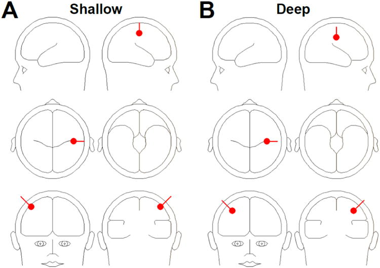
Location and orientation of a representative dipole generator underlying scalp location C4, as shown by Dipole Generator (Berg, 2006) in lateral (left and right), horizontal (top and bottom) and coronal (front and back) views. Scalp electrode placements were defined for a 67-channel scalp montage using the extended 10-20 system coordinates (Jurcak et al., 2007), and registered to the four-shell spherical head model of Dipole Simulator (Berg, 2006). Radial dipole generators were then pos itioned at either (A) shallow (2 mm subdural) or (B) deep (15 mm subdural) locations.

For each dipole, a forward solution was computed for a unit amplitude generator at a single time point (10 nAm source waveform; 3-point triangle waveform). The resulting field potential topographies were then saved as a topography vector using a fixed reference scheme (nose reference). These vectors were applied to sinusoidal source waveforms (2 s × 256 samples/s; 10 Hz sine or cosine, as required) in Matlab for each of the dipoles required in a specific generator model (as detailed below). Because volume conduction is itself linear, the final scalp potential topographies for multiple generators were constructed as the sum of the individual dipole topographies, resulting in a single simulated EEG scalp record (67 channels × 512 points; nose reference [NR]).

By virtue of these methods, all of the imposed and measured signals are sinusoidal waveforms, each with a characteristic amplitude and phase that may be directly measured from the timecourse of the signal. These temporal signals may then be linearly transformed to observe the impact of rereferencing and SL transformations, which also yield sinusoidal waveforms with identifiable amplitudes and phases. However, equivalent measures of amplitude and phase may be quantified directly from their complex Fourier Transform pairs (e.g., Smith, 1997). Likewise, rereferencing and SL transformations may be performed following, rather than preceding, the FFT owing to the fact that the complex FFT is a reversible linear transformation¹.

2.2. Generator models

2.2.1. Model 1

The first model was intended to establish the properties of individual dipolar oscillatory generators with sufficient separation to allow their unambiguous separation by different field potential and surface Laplacian transformations. It consisted of superficial cortical dipoles at depths corresponding to mid-to-deep laminae of superficial cortex (i.e., 2 mm below surface of dura). Two standard 10-20 sites were selected corresponding to focal generators at right central (cosine at site C4) and right parietal (sine at site P4) scalp locations, providing a comparison of the amplitude and phase at ‘active’ (i.e., C4, P4) sites, and their spread due to volume conduction at ‘inactive’ sites (all other 65 sites of the EEG montage). Likewise, an identical pair of dipoles was placed at deep cortex locations directly under these scalp sites, 15 mm below dura.

2.2.2. Model 2

The second model probed the adequacy of the same transformations to separate and describe the amplitude and phase properties of contiguous generator regions at posterior areas of one hemisphere. It consisted of a series of superficial cosine generators distributed below six extended 10-20 scalp sites in the right posterior cortex (Pz, POz, P2, P4, PO4, P6), and sines below two adjacent scalp sites (P8, PO8).

2.2.3. Model 3

The third model was constructed to approximate minimal properties of posterior condition-dependent EEG alpha. Superficial generator regions were considerably larger, with dipoles distributed below 30-posterior electrodes spanning postcentral sites in both hemispheres. Cosine generators included the entire left hemisphere and midline, as well as some right hemisphere sites (TP9, TP7, CP5, CP3/4, CP1/2, CPz, P9, P7, P5, P3/4, P1/2, Pz, PO7, PO3/4, POz, O1, Oz), with sine generators below the eight remaining sites (CP6, TP8, TP10, P6, P8, P10, PO8, O2). Gaussian noise (desribed below) was also added to allow the comparison of coherence for each of the transformations.

2.3. Data transformations

2.3.1. Fourier transformation

Spectral transformation of each of the sinusoidal stimuli used in these simulations (i.e., cosine and sine waveforms at a single frequency) results in a trivial spectrum: a single nonzero complex amplitude at 10 Hz. To avoid redundancy and further simplify the analyses, only the NR simulations were subjected to FFT. Field potentials were rereferenced and surface Laplacian estimates computed from these complex topographies.

2.3.2. Field potential reference strategies

Simulated NR scalp potential waveforms were transformed to create waveforms for two additional field potential references: common average reference (AR) and linked mastoid reference (LM; TP9/10).

2.3.3. Surface Laplacian estimates

Spherical spline Laplacian (Current Source Density, CSD) estimates were computed with the widely-used method of Perrin et al. (1989; Kayser and Tenke, 2006a; Kayser, 2009). Our standard parameters have proven useful for group averages in previous ERP and EEG studies (smoothing lambda = 10^-5; 50 iterations; moderate spline flexibility m = 4; cf. Kayser and Tenke, 2015b, and are identified here as CSD₄ (i.e., subscript identifies spline flexibility). Laplacian estimates based on additional spline flexibilities (i.e., CSD₂-CSD₅) were also computed to evaluate the impact of this parameter on accuracy and spatial scale when compared to field potentials.

2.4 Amplitude and phase comparisons

2.4.1 Accuracy measure

For each model and three transformations (CSD₄, NR and AR), an amplitude accuracy estimate was computed based on conformation of each simulated topography to the radial positions of the simulated dipoles using unit amplitudes scaled to the shallow maximum of each transformation. For Model 1, the “correct” locations corresponded to electrode sites C4 and P4, for which the accuracy estimate equaled the observed amplitude value (A) at each of these sites. Other “incorrect” locations were coded as 1-A, resulting in a possible range between 0 and 1 for each site. These amplitude accuracy estimates were then submitted to an ANOVA with transformation (CSD₄, NR and AR) as a repeated measure, using the 67 sites as observations. Analoguous estimates were computed for CSD3 and CSD5 to also compare SL estimates derived from spherical splines of different flexibility with field potentials in an ANOVA employing a 4-level repeated measures factor transformation (NR, CSD₃, CSD₄, CSD5). Significant transformation main effects (Greenhouse-Geisser correction) were followed-up by pairwise contrasts (BMDP-4V; Dixon, 1992).

2.4.2. Models 1 and 2

The first two models have the advantage of a precise, noise-free sinusoidal generator, making it possible to directly compare the phase of the temporal generator waveforms and the resulting reference-dependent and SL waveforms. Since they were noise-free, a secondary goodness-of-fit estimate is unnecessary and inappropriate. However, the raw temporal waveforms (all sinusoids) were most readily compared using a Fast Fourier Transform (FFT) for comparison of spectral amplitudes and phase. For each reference (NR, AR, LM) or SL transformation (m = 3, 4, 5), the waveform at each electrode was completely described by the 10 Hz component, the amplitude being its complex amplitude and the phase its complex phase. These measures were compared across transformations to identify and describe differences for these idealized signals.

2.4.3. Model 3

The third model allows the examination of phase stability as measured by coherence, which, by analogy with the product-moment correlation coefficient, requires multiple, nonidentical estimates to provide a meaningful estimate. To accomplish this, the original 512-point record for each electrode in the montage was replicated for 1000 virtual epochs that were successively shifted by 360E/1000 (i.e., phase drift of one cycle over trials). Based on the maximal amplitude observed for the NR topography, Gaussian noise with a standard deviation of .005, .05, or .5 was separately added at 10 Hz (i.e., peak frequency) to the real and imaginary FFT components². The resulting waveforms were then rereferenced to NR, AR and LM [(TP9+TP10)/2] and Laplacian transformed using m = 2, 3, 4, and 5. Following Bendat and Piersol (1971), cross spectra and power spectra estimates were then computed, averaged across the 1000 virtual epochs, and summarized as amplitude spectra and coherence (for each pair, the squared cross spectrum [i.e., spectral covariance] divided by the product of each power spectrum [i.e, spectral variance]). Regional coherence estimates were also computed from cross- and power spectra computed for each of the two posterior regions (i.e., 22 and 8 electrodes, excluding identity coherences). Coherence measures were expressed following a square root operation to yield the familiar product-moment correlation coefficient, and also to scale the data for mapping.

3. Results

The amplitudes and phases for each transformation at each electrode site are precisely measurable for Models 1 and 2. Accordingly, comparing the locations and distribution of the amplitude maxima and the differences between observed phase angles is a sufficient description of the findings.

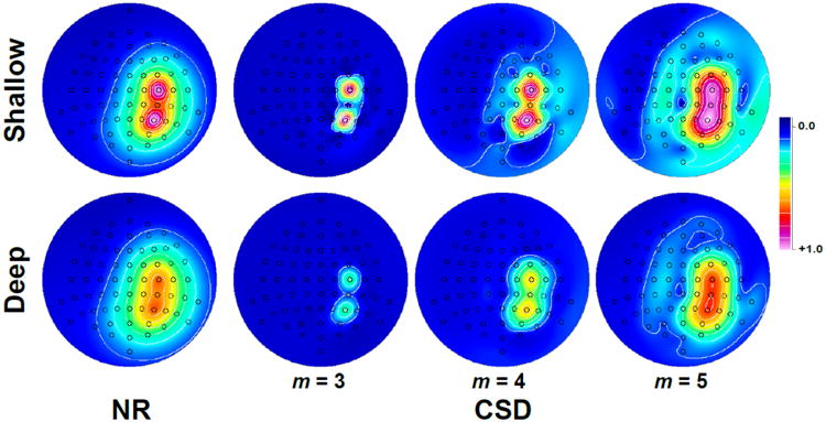
Fig. 2 shows the amplitude topography of the 10 Hz spectral peak corresponding to the pairs of 90E phase-shifted sinusoidal radial dipoles below sites C4 and P4 in Model 1. The NR and AR field potential topographies are remarkably focal for the superficial generator. However, the amplitude measured at intermediate sites CP2 and CP6 (i.e., nearby, but not radial) is considerably smaller for CSD (m = 4), consistent with a falloff from the two active sites (Fig. 2A). This superiority is preserved for deep sources, for which NR amplitude midway between active sites (CP4) is no longer distinguishable from that at the active sites (i.e., C4 and P4).

Fig. 2.

Model 1. Map of peak of amplitude spectrum (FFT amplitude at 10 Hz) for nose-referenced (NR), average-referenced (AR) EEG and surface Laplacian (CSD; m = 4) derived from a pair of 90 degree phase-shifted sinusoidal radial dipoles localized to sites C4 and P4. A. EEG and CSD topographies for shallow and deep generators. The top two rows were scaled to yield a unit amplitude corresponding to the shallow maximum (i.e., same scaling factor for shallow and deep, but different for NR, AR and CSD). The bottom row shows the deep generator topographies scaled to unit amplitude for each map, emphasizing the topographic superiority of CSD for deep generators. All topographies in this report are two-dimensional representations of spherical spline interpolations (m = 2; λ = 0) derived from the values (i.e., amplitude, phase angle) available for each recording site, at which quantified data are precisely represented. B. Amplitudes at each scalp site as shown in A, sorted by descending order observed for shallow NR (i.e., from left to right, starting with maximum values at P4 and C4). The vertical line indicates the separation between active and inactive (volume-conducted) sites.

The amplitude falloff across the topography for NR and AR EEG and the corresponding CSD are directly compared in Figure 2B³. Reference-dependent EEG topographies indicate considerably greater amplitudes across inactive portions of the topography (“false positives”) than do CSD topographies. The AR has a falloff that is intermediate between the NR and the CSD, but abruptly degrades with distance, beyond which it consistently overestimates activity (i.e., subsequent rise to .2 amplitude).

When compared to a shallow source, a deep source results in a noteworthy attenuation and topographic shift in both reference-dependent EEG and CSD measures (Fig. 2B). The NR peak is attenuated by 33%, but its topography is otherwise comparable to that of the shallow generator, thereby obscuring the active-to-inactive transition (at CP4). Although the CSD shows a stronger attenuation (47%), the distinction between active and inactive sites is better preserved. The AR has an intermediate attenuation (42%) at active sites, but is essentially unchanged over most of the topography, owing largely to topographic distortions unrelated to volume conduction.

The topographies produced by superficial and deep generators can be more readily compared by scaling each individual map (Fig. 2, bottom row). Although all measures show reduced selectivity for active sites in the case of the deep generator, NR shows a dramatic reduction in selectivity compared to the shallow source (i.e., exhibiting a gradual decline across all sites). Moreover, despite an observable flattening of CSD falloff, the specificity of the CSD topography is much better preserved than either of the reference-dependent measures. The AR is again intermediate in performance near the active sites, and suffers from a severe overshoot from the computational artifact, providing the worst topographic estimates at a distance (i.e., the entire left hemisphere).

Table 1 summarizes the findings for the amplitude accuracy estimates for all models, with each revealing robust effects of transformation. For both shallow and deep generators of Model 1, CSD accuracy was greater than NR and AR. This measure is clearly affected by the spread introduced by volume conduction (Fig. 2, NR) and computational artifact (Fig. 2, deep AR). Surprisingly, the difference between CSD and the two field potential transformations was even greater for deep than shallow sources, which was confirmed in a post-hoc ANOVA for Model 1 with depth (shallow, deep) as an additional repeated measure factor (depth × transformation interaction, F[2, 132] = 28.7, p < .0001, epsilon = 0.58044).

Table 1. Means (±SD) of amplitude accuracy estimates (across all 67 sites) by generator model for each transformation and ANOVA F ratios.

		Model 1				Model 2		Model 3
Simulated sourcea		Shallow		Deep		Shallow		Shallow
CSD4		0.88	±0.14	0.90	±0.11	0.89	±0.09	0.71	±0.19
NR		0.82	±0.17	0.80	±0.16	0.82	±0.17	0.78	±0.15
AR		0.81	±0.11	0.80	±0.10	0.77	±0.11	0.62	±0.20
Effect b		F	p	F	p	F	p	F	p
Transformation c		18.0	<.0001	44.2	<.0001	20.3	<.0001	14.1	<.0001
Contrasts	NR-CSD	34.4	<.0001	67.9	<.0001	24.3	<.0001	7.38	.008
	AR-CSD	34.7	<.0001	153.4	<.0001	46.0	<.0001	8.07	.006
	AR-NR					3.89	.053	23.9	<.0001

^aCSD₄: current source density, m = 4; NR: nose reference; AR: average reference.

^bFor all effects, df = 1, 66. Only F ratios with p < .10 are reported.

^cGreenhouse-Geisser adjusted df, 0.69097 ≤ ε ≤ 0.89650.

Fig. 3 A illustrates the phase measured for the shallow simulations shown in Fig. 2. NR and AR both show a reduction in the 90E phase difference between active sites (P4 and C4), with NR showing the smallest difference. In contrast, CSD (m = 4) phase differences are increased by an amount comparable to the decrease for AR. Notably all measures show a phase null (i.e., midpoint between 0E and 90E) at the nearest inactive site (CP4). For the deep generator, the results are unambiguous: the phase differences were precisely preserved by the CSD, but distorted (strongly attenuated) for the reference-dependent EEG, being worse for NR than AR.

Fig. 3.

Model 1. Peak frequency phase angle (degrees) for (A) shallow and (B) deep generators at electrodes with greatest shallow NR amplitude (>.35; sorted by NR; cf Fig. 2B). Electrodes in shaded areas are radial to dipole generators (i.e., active regions)

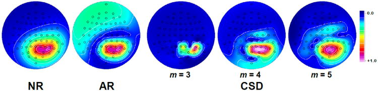
As shown in Fig. 4A and C, the scaled amplitude topographies for Model 2 are comparable across data transformations in active regions, being smaller at both the medial (Pz, POz) and lateral (P8, PO8) edges of the region. There was no prominent distinction between subregions having different phase properties in any of the topographies. However, the transition between active and inactive sites was again most abrupt for the CSD, and least for NR. The AR was again intermediate at this transition, but abruptly degraded across the montage, where the reference calculation misallocated a considerable amount of activity to inactive sites (see left frontal sites in column 2 of Fig. 4A). These observations were supported by the statistical findings for the accuracy measure for Model 2, which revealed that CSD accuracy was greater than NR and AR, and NR was marginally greater than AR (Table 1) As in Model 1, the effect appears to be related to the spread introduced by volume conduction for NR, and to the computational artifact for AR.

Fig. 4.

Model 2. Peak amplitude spectrum (FFT amplitude at 10 Hz) for NR and AR EEG and CSD (m = 4) derived from two contiguous regions composed of 90 degree phase-shifted, shallow radial sinusoidal dipoles. A. Although all amplitude topographies show a distributed maximum within the (combined) active regions, the border for the CSD topography is considerably sharper. The AR has an intermediate falloff, but misallocates activity to distant inactive sites (i.e., left anterior). Each data set is individually scaled to 1. B. Schematic to indicate locations of active regions. Region 1 (red dots) contains shallow radial cosine dipoles at six posterior sites (Pz, POz, P2, P4, PO4, P6). Region 2 (blue dots) is immediately adjacent to region 1, and contains shallow radial sine dipoles (P8, PO8). C. Amplitude at each electrode shown A, sorted by NR amplitude. The dashed vertical line at the left separates active from inactive (volume conducted) electrodes, the dashed horizontal line marks half the maximum amplitude. Again, CSD amplitude shows the sharpest falloff between active and inactive sites. D. Peak phase at active (shaded) and adjacent sites, sorted as in Fig. 4B. The maximum phase difference between Region 1 and Region 2 exceeds 65E for CSD. NR shows the smallest phase difference between regions, with the AR intermediate between them.

The phase difference between the generator regions was fixed at 90E in the simulation. These phase properties were not accurately preserved for any of the measures (Fig. 4D). However, the phase differences observed for the CSD were considerably better than those observed for either of the reference-dependent EEG measures, being closest for the most distant sites (Pz, POz, P2 vs. P8, PO8), but shifting in phase across intervening sites (P4, PO4, P6) as the transition between generator regions was approached. While the corresponding phase differences between regions were better preserved for AR than NR, if this had been empirical data, the misallocation of power to anterior sites by the AR would increase the likelihood that these meaningless phase properties would likely have been recognized and reported.

Fig. 5 shows the impact of spline flexibility on CSD estimates for superficial and deep focal generators of Model 1. It is clear that a greater spline flexibility results in a more precise spatial localization of active sites, but at the expense of attenuation with depth. Conversely, more rigid splines preserve amplitude estimates of deep generators even better than the untransformed EEG, but also blur the topography, even for superficial generators.

Fig. 5.

Impact of spline rigidity on CSD amplitude estimates (lambda = 10^-5) of Model 1 shallow and deep focal generators in comparison to NR. A more flexible spline (m = 3) leads to a more precise localization of generators, but at the expense of further attenuation with depth. Conversely, a stiffer spline (m = 5) results in less attenuation than the untransformed NR EEG, but oversmooths shallow generators.

Given that NR showed better amplitude accuracy estimates across all models compared to AR (Table 1), NR was compared for this measure to three CSD estimates using either flexible, medium or rigid splines (m = 3-5). These findings are summarized in Table 2. Again, but to a different degree, all models revealed significant transformation effects. For Model 1, shallow generators were best represented by CSD₃, followed by CSD₄, NR, and CSD₅, all being significantly different from each other. Deep generators for Model 1 were also best represented by CSD₃, followed by CSD₄, however, the following lower accuracy estimates did not differ between NR and CSD₅, thereby confirming the observation of highly similar topographies between NR and CSD₅ for these deep sources (Fig. 5, bottom row, columns 1 and 4).

Table 2. Means (±SD) of amplitude accuracy estimates (across all 67 sites) by generator model comparing nose-referenced field potentials (NR) and CSD estimates for different spline flexibilities (m = 3-5) and ANOVA F ratios.

		Model 1				Model 2		Model 3
Simulated source a		Shallow		Deep		Shallow		Shallow
NR		0.82	±0.17	0.80	±0.16	0.82	0.17	0.78	0.15
CSD3		0.98	±0.02	0.96	±0.12	0.91	0.19	0.72	0.18
CSD4		0.88	±0.14	0.90	±0.11	0.89	0.09	0.71	0.19
CSD5		0.76	±0.76	0.81	±0.16	0.85	0.12	0.73	0.17
Effect b		F	p	F	p	F	p	F	p
Transformation c		57.7	<.0001	53.3	<.0001	7.36	0.002	3.69	0.02
Contrasts	NR-CSD3	65.9	<.0001	58.2	<.0001	8.70	0.004	5.20	0.03
	NR-CSD4	34.4	<.0001	67.9	<.0001	24.3	<.0001	7.38	0.008
	NR-CSD5	31.4	<.0001			6.75	0.01	4.97	0.03
	CSD3-CSD4	36.9	<.0001	29.5	<.0001
	CSD3-CSD5	70.2	<.0001	51.9	<.0001	4.73	0.03
	CSD4-CSD5	55.6	<.0001	66.8	<.0001	14.8	0.0003

^aNR: nose reference; CSD_{3 5}: current source density, m = 3 .. 5;

^bFor all effects, df = 1, 66. Only F ratios with p < .10 are reported.

^cGreenhouse-Geisser adjusted df, 0.42053 ≤ ε ≤ 0.75442.

Fig. 6 shows the impact of spline flexibility on CSD estimates of the simulated distributed generator. The superiority of a CSD using an intermediate spline flexibility (m = 4) appears quite clear, although at the cost of adding erroneous amplitudes at adjacent sites compared to the more flexible CSD₃,while a less flexible spline (m = 5) increased the measured spread of activity to surrounding sites nearest to the generator region (i.e., comparable to AR, but without left anterior activity). In contrast, the application of a more flexible spline (m = 3) resulted in errors that underrepresented amplitudes for most of the active region, and represented activity near the center of the generator region (i.e., at P4) as a null (cf. Fig 4B). These observations largely corresponded to the statistical findings, although CSD₃ and CSD₄ did not differ significantly and actually CSD₃ showed larger means than CSD₄ in this amplitude accuracy measure. Both CSD₃ and CSD₄ were superior to NR and CSD₅, the latter being somewhat better than NR (Table 2).

Fig. 6.

Impact of spline rigidity on CSD amplitude estimates (lambda = 10^-5) of Model 3 distributed generators in comparison to NR and AR. Although the moderately stiff spline (default; m = 4) was effective for this widely distributed generator, a flexible spline (m = 3) strongly attenuated amplitudes, and yielded null at P5 (near the center of the region). Conversely, a stiffer spline (m = 5) smooths the transition between active and inactive regions.

Spline flexibility had a strong impact on phase measured across the active region for Model 2. The CSD phase for the less flexible spline (m = 5) paralleled that of the standard CSD across the large generator region 1, but was comparable to NR for the small one. However, for a more flexible spline (m = 3), almost all phase measures were within 5E of the simulated signal (i.e., either zero or -90E), with the single exception being at P4, where the CSD amplitude showed an amplitude null. The CSD phase estimate at this site, as well as at adjacent inactive sites (O2 and CP6; CSD amplitudes <.05), was not measurable (69, 154 and 163E, respectively).

The amplitude and phase properties of the broad posterior generator regions of Model 3 are shown for all references (NR, LM and AR in Fig. 7B) and for CSD estimates (m = 2-5) in Fig. 7C. All three field potential measures identify the larger generator region over the posterior left hemisphere, but differ in their representation of the smaller region over the right hemisphere. AR shows a somewhat greater, and LM less separation between regions than NR. A point worth noting is that the mastoids (TP9/10) are not quiescent in this simulation, which accounts for their amplitude elevation above zero (cf Fig. 7A) and the amplitude minima at the outer border of the two regions at central sites (near C4) and near the inion (Iz). These differences were probed for CSD₄, NR and AR using the accuracy measure tests (Table 1). For Model 3, CSD accuracy was greater than AR, but NR was greater than CSD and AR. As in Models 1 and 2, the poorer performance of AR was clearly related the anterior computational artifact. However, the decreased performance of CSD₄ for Model 3 was a consequence of the relative attenuation at sites within the generator regions (cf. Fig. 7, NR vs CSD₄ amplitude topographies). Notably, spline flexibility had little if any effect on these amplitude accuracy estimates (i.e., no significant differences between CSD₃, CSD₄, and CSD₅), while NR was better than any of the CSD estimates for this broadly distributed, posterior generator source, although these differences were moderate compared the other significant differences listed in Table 2.

Fig. 7.

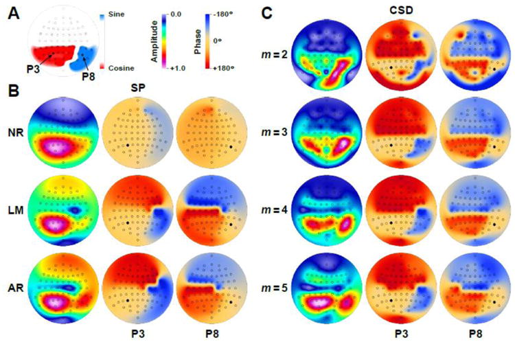
Amplitude and phase topoghraphies obtained for Model 3 without noise. A. The locations of the two posterior generator regions in association with the scalp sites at which they were measured via forward solution. A sine wave was simulated at all subdural dipoles in the smaller, right hemisphere (blue) region, and a cosine wave at all other generator sites (red region). Sites P3 and P8 (10-20 nomenclature, Pivik et al., 1993) located in the respective centers of sine and cosine regions are identified to simplify phase comparisons. Note that these two sites are set to zero phase angle, and as a consequence, the phase angle shifts across all other sites as plotted towards ±180 ° inform about their origin when map pairs are considered jointly. B. Column 1: Surface potential (SP: NR, LM, AR) amplitude topographies scaled to 1 to facilitate comparisons. Columns 2 and 3: SP phase angles as differences from site P3 and P8. C. Corresponding amplitude and phase CSD topographies computed using different spline flexibilities (m = 2-5).

Due to the fact that phase angles are unique only within ∀180E, they may be difficult to interpret when multiple generators exist. In the present model, there are only two active regions, the wider of which having an explicit phase relationship to the second (i.e., 0E [cosine] vs. -90E [sine]). To fix this relationship for each transformation, the phase at each site was rezeroed to the measured phase within this larger region at electrode site P3, and within the smaller region at site P8, thereby maximizing the range of the scale before the phase crossover. As a consequence, the direction of the phase angle shifts across all other sites, including those close to ±180°, provide information about their origin when map pairs are considered jointly.

These phase topographies are shown in Fig. 7 (cf. red-orange-blue color scale), adjacent to the corresponding amplitude topographies for each transformation. It is immediately apparent that the phase of posterior regions for NR varies smoothly across the topography, although the 90 degree shift between regions was understimated (56E). The posterior phase topographies of AR and LM are also consistent with NR within the reference generator region (i.e., at or near P3). However, at sites beyond the anterior edges of the generators, AR and LM both show phase shifts far in excess of the 90E difference that was imposed (i.e., >100E difference; dark blue extrema for P3, dark red extrema for P8). This is presumably attributable to the inclusion of active sites in the reference, the subtraction of which is equivalent to the inclusion of activity shifted by 180E.

The NR hemispheric phase asymmetry observed near the posterior generator sites continues to anterior sites as well, which is not problematic because the amplitude drops to near zero at these locations. In contrast, AR and LM both show an abrupt phase shift at ∀180E immediately anterior to the region contralateral to the phase-zeroed site (right extrema blue for P3; left extrema red for P8). The amplitudes at these sites range from zero (i.e., the phase is irrelevant) to .4 for LM and .6 for AR. Moreover, their measured phase remains almost precisely out of phase compared to the larger, left hemisphere generator for most anterior regions as well (i.e., dark red for P3; light blue for P8). Not surprisingly, these sites include the secondary amplitude maximum near the frontal pole, which is consistent with a subtraction of the dominant (cosine) waveform from these sites due to referencing.

The amplitude topographies characterizing the CSD varied considerably depending on spline flexibility (right side of Fig. 7). With less flexible splines (m = 4 and 5), both regions were represented in proportion to their size. In contrast, more flexible splines (m = 2 and 3) poorly represented the size of the larger generator region, localizing the smaller, right hemisphere region best. Although no anterior activity was evidenced by either of the more flexible splines, anterior amplitudes for the less flexible (m = 4 and 5) were nonzero, albeit considerable less than AR and LR.

Mean regional phase differences were also overestimated for CSDs, but systematically varied according to spline flexibility (m = 2, 115E; m = 3, 109E; m = 4, 103E; m = 5, 98E). The phase across the larger, left hemisphere region was approximately zero (P3 phase) for all but the most flexible splines (m = 3, 4 and 5). Moreover, the phase transition between the two regions was precisely identified by CSD with m = 3 (compare blue-to-orange transition of CSD₃ P3 phase; red-to-orange transition for P8). Although phase maps for all CSDs suggest that anterior sites are 180E out of phase with the left hemisphere generator (i.e., dark red for P3; light blue for P8), their occurrence at sites with near-zero amplitudes make them irrelevant (in stark contrast to AR and LM).

In comparison to the other CSD estimates, the most flexible spline (m = 2) produced the most irregularities for sites within the generator regions. While the amplitude topography of the larger, left hemisphere region was reduced to <.5 over most of its surface, the amplitude of the smaller region was sharpened and spatially shifted, with its greatest amplitude appearing not over the generator, but rather over the phase inversion. Zero amplitudes also occurred in conjunction with +90 degree phase shifts at sites POz and P10. However, the appearance of larger negative phases (#-90E) within the smaller, right hemisphere region and larger positive phases (>90E) within and around the larger region suggested at the ∀180E phase crossover distorted the appearance of the underlying phenomenon. Both CSD₂ and CSD₃ both yielded phase contrasts at the border between regions, and for all flexibilities between generator regions and frontal inactive regions.

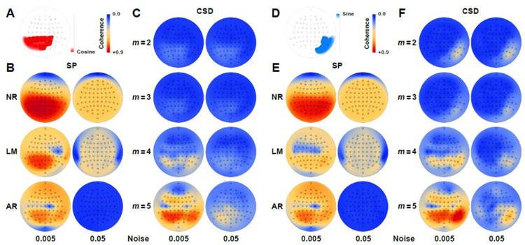
The impact of Gaussian noise on these amplitude topographies is shown in Fig. 8. All three of the field potential transformations retained their structures with low noise (.005), but were dominated by noise at the higher noise level (.05), where only the reference site(s) are evident for NR and LM. In contrast, the amplitude topography of the CSD was preserved with noise only for the rigid spline (m = 5), but was degraded (m = 4) or obliterated (m = 2, 3) by flexible splines. The highest noise level (not shown) only yielded topographies representing the noise, and will not be further discussed.

Fig. 8.

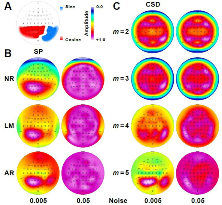
Model 3. Amplitude topographies of surface potential (SP; B) and CSD estimates (C) at low (.005) and higher (.05) noise levels, scaled to their maxima. Generator regions are shown in A. With low noise, field potential topographies closely parallel those without noise (cf. Fig 7B). In contrast, the only CSD estimate that was not degraded by low noise was the one computed using the most rigid spline (m = 5).

Despite the severe impact of noise on the amplitude topographies, pairwise electrode coherence topographies anchored at scalp sites overlying the generator regions of Model 3 paralleled the noise-free amplitude topographies for all field potential measures and for the least flexible spline CSD₅, but not for more flexible splines. Conversely, pairwise coherence topographies anchored at electrodes near the frontal pole (FP1/2, FPz, AFz) for AR and LM, but not NR, indicated nearly perfect coherence both with posterior (“active”) and anterior (“inactive”) sites.

Figure 9 A indicates the scalp location of the large (cosine) generator region spanning the posterior left hemisphere in Model 3. The regional coherence topographies obtained for field potentials (NR, LM and AR) across this region are shown in Fig. 9B. Low-noise topographies (.005) paralleled the corresponding amplitude topographies (cf Fig.8). NR showed the largest posterior coherence maxima and the greatest falloff near the frontal pole (blue region). In contrast, the other reference transformations suggested at anterior activity (orange regions), rather than a falloff, particularly for AR near the frontal pole (dark orange regions). At greater noise level (.05), coherence based on field potentials did not showed meaningful topographies apart from minima corresponding to their respective references (nose for NR; mastoids for LM; overall topography for AR).

Fig. 9.

Model 3. Regional coherence topographies at low (.005) and higher (.05) noise levels for field potentials and CSD estimates. A. Identification of larger cosine region. B. Surface potential (SP: NR, LM, AR) coherence topographies with low noise (.005) computed across the larger cosine region paralleled amplitude topographies without noise (cf. Fig. 7B). At higher noise levels, coherence levels dropped dramatically, and were eliminated in proximity to the recording reference (nose for NR; mastoids for LM; entire topography for AR). C. Corresponding regional coherence CSD (m = 2-5) topographies, which retained their organization only for rigid spline (m = 4, 5) at low noise levels. D. Identification of smaller sine region. E. Field potential (NR, LM, AR) coherence topographies at low noise included an enhanced contribution of the small generator region itself, imposing an asymmetry into the topography (cf. B). Regional coherence for the high noise level was undifferentiated, as described for the large cosine region (cf. B). F. Corresponding CSD topographies, which preserved their spatial structure with low noise for rigid splines (m = 4 and 5), while also introducing an asymmetry with a maximum over the smaller generator region. At high noise levels, the topography for the most rigid spline (m = 5) retained a right-lateralized topography.

Figure 9D and E show the corresponding scalp locations and regional coherence topographies for the smaller right (sine) generator region in Model 3. Again, the low-noise topographies paralleled their corresponding amplitude topographies. A comparison of the regional coherence topographies for the two regions (B vs. E) also indicated a hemisphere selectivity for LM coherence with low noise (i.e., less red over left and more orange over right hemisphere in E). NR showed a trend toward a this asymmetry (slightly more red over right hemisphere in E than B), but AR did not.

For CSD estimates, regional coherence topographies with noise (Fig. 9C, F) also paralleled their corresponding amplitude topographies. Notably, only the most rigid splines (m = 4, 5) yielded clear posterior topographies. Although CSD₅ provided the best representation of the posterior generator regions, it also indicated coherence immediately anterior to the generators. CSD₅ also showed marked asymmetries (i.e., left hemisphere for Fig. 9C; right hemisphere for 9F). Not surprisingly, CSD coherences were reduced for when the level of noise was high (.05). However, coherences across the smaller, right hemisphere region (Fig. 9D) were still considerable (>.4) for high noise with CSD₅.⁴

4. Discussion

4. 1. Overview of Simulations

CSD provides a minimal description of the neural current generators underlying a scalp-recorded EEG topography, and any inverse solution that disagrees with the pattern of scalp sources and sinks cannot be valid (Tenke and Kayser, 2012). Despite this tautology, different algorithms yield surface Laplacian estimates that differ in their spatial tuning. Methodological approaches that aim to closely approximate an analytic Laplacian solution have led to the identification of the approach as a high-resolution EEG method, and have consequently delegated its use to high density recording montages (Junghöfer et al., 1997). Conversely, in order to identify physiologically meaningful patterns of sources and sinks from some phenomena, it may be appropriate, or even required, to use Laplacian methods with a lower spatial resolution (MacFarland, 2014; Tenke et al., 1993; Tenke and Kayser, 2012).

This report provides strong support for the reliable application of CSD methods to oscillatory brain activity. They also suggest that some of the apparent weaknesses of CSD when compared to reference-dependent EEG measures may result from a misunderstanding of their intracranial origins. These observations do not refute conventional concerns about the complementarity of high- and low-resolution EEG methods, but rather the understanding that Laplacian methods are inherently high-resolution. Owing directly to the use of surface Laplacian methods in image processing as an edge-detector, there is an a priori presumption in the field that deep or distributed generators are universally problematical for them, even when such errors cannot be identified in empirical data (Kayser and Tenke, 2006a; Tenke and Kayser, 2005, 2012). The present simulations were aimed at mitigating these concerns.

Model 1 was restricted to a pair of superficial and deep dipole generators, and thereby provided a simple heuristic starting point for illustrating the implications of volume conduction on the measurement of the amplitude and phase of oscillatory generators. For Model 1, CSD computed with a moderately flexibile spline (m = 4) had a sharper spatial falloff at sites nearest the generators than the reference-dependent measures, which was associated with greater accuracy measures. The falloff for AR was intermediate, but the topography included a computational artifact that dominated distant regions of the topography. Phase differences were also between preserved for CSD above each dipole, as well as at nearby sites. Not surprisingly, the performance of CSD was improved by the use of a more flexible spline (m = 3). Model 2 expanded on this model by simulating a distributed superficial generator below eight adjacent posterior sites. CSD₄ again outperformed the field potential measures both in topography and accuracy, but AR accuracy was poorer than NR, owing to the increased computational artifact at anterior sites for these posterior sources. However, while CSD with the least flexible spline yielded lower accuracy scores than CSD₃ and CSD₄, the latter could not be distinguished from each other statistically. The 90° phase shift between regions in Model 2 was attenuated for all measures, but was appeared to be best preserved by CSD₄, and worst for NR.

Model 3 provided a considerably greater challenge for CSD, because it was the most broadly distributed model and spanned all posterior scalp locations. Despite its shallower falloff, the amplitude topography of NR yielded a better accuracy than CSD₄, owing to the sharp separation of the two generator regions by the CSD. Again AR performed worst, owing to the prominent computational artifact in frontal regions. Variations in spline flexibility strongly influenced the spatial tuning of the CSD for Model 3. The most flexible splines (m = 2 and 3) preferentially represented the smaller of the two regions (sine, right hemisphere), while most rigid spline (m = 5) represented the larger one (cosine, left hemisphere). This clear topographic shift was not reflected by the global accuracy measures; CSD were all poorer than NR. Phase representations above generator regions were generally good for Model 3. The 90° phase shift between regions was reduced for NR. However, it was preserved for AR, LM and CSD for all but the most flexible spline (m = 2); as was the relative phase inversion at anterior sites. The implication for AR (and to a lesser extent, LM) had substantial inverted anterior activity, while for CSD it was negligible.

The addition of noise to Model 3 was also informative. Although high noise levels disorganized the amplitude topographies for all transformations, low levels of noise resulted in amplitude topographies for NR, LM and AR which were similar to their noise-free counterparts. In contrast, only the CSD with the most rigid spline (m = 5) yielded a plausible amplitude topography. Consistent with these findings, the corresponding regional coherence topographies suggested associations within and between generator regions for all field potential measures, but only for CSD₅. Spurious coherence with anterior sites was likewise greatest for AR.

With the appropriate selection of computational parameters, Laplacian methods were shown to yield results that are competitive with reference-dependent field potential strategies in detecting broadly distributed activity, but better at characterizing their underlying generators. All referenced field potential strategies risk the possibility of artifactual, nonphysiological conclusions for amplitude or power topographies. This concern also applies to the AR, and requires clarification. There is no controversy over the reversibility of EEG topographies and their corresponding complex frequency spectra. A field potential topography can be rereferenced in either domain. What is often neglected is that the complex-to-real conversion required to produce amplitude or power spectra is itself irreversible (cf Fig. 1 in Tenke and Kayser, 2005). For all models, but Model 3 in particular, AR must decrease the maximum amplitude of the posterior topography, but also subtract activity equally from anterior sites. While the resulting inversion of anterior waveforms is numerically trivial, the associated phase shift risks misinterpretation as evidence for a frontal generator, particularly when noise is present to further mask its origin.

4.2 Relevance of simulations to empirical measures

A variety of approaches have been used to simulate the simultaneous recording of a montage of sinusoids differing in phase and/or noise. In one approach, signals and noise are linearly combined to simulate activity at electrodes on a scalp montage, and the results are compared for different reference strategies (Thatcher, 2012). This simple approach is sufficient for scalp potentials because the rereferencing transformation is linear, reversible, and requires no spatial information; any arbitrary signal can be presumed at any given electrode with impunity. However, this luxury is not possible for a more realistic model, and therefore not for a surface Laplacian. In a volume conduction model (Nunez and Srinivasan, 2006), all sources affect all electrodes, so that a poorly chosen signal strength at any location could imply a sharply localized, partially closed field (Tenke and Kayser, 2012), which in turn would (correctly) imply the existence of unintended current-closing CSD features (Tenke et al., 1993). Regardless of whether they appear as discrepancies in amplitude or in phase, the origin of these artifacts lies not in the Laplacian, but in an implicit inconsistency with the requirements of volume conduction.

Our simulations avoided these problems by using a well-defined four shell volume-conductor head model. They also incorporated some fundamental simplifications: 1) the waveforms were true sinusoids; 2) activity was simulated only as a single frequency; 3) the phase properties of the generator were precisely defined, rendering their measurements at each electrode exact; 4) the generators were positioned radially at fixed subdural locations in superficial cortex. The final model added uncorrelated Gaussian noise to each electrode to allow a meaningful estimation of coherence. Since these constraints are not present for empirical electrophysiological recordings, their implications have to be taken into account in the context of empirical spectral measures.

4.2.1 Implications of restricted spectrum

By restricting activity to sinusoids at a single frequency, the transformation between time and frequency becomes trivial, as well as reversible (i.e., prior to simplification as amplitude spectra). In fact, if any other spectral activity had been detected, it would have provided conclusive evidence of a computational error. Although the same argument is also applicable to the phase of a signal, the impact of volume conduction may be less apparent. Thus, for isolated radial dipole pairs, the observed phase of the waveforms directly reflected the phase imposed at the nearest radial electrode (i.e., 0E or -90E). However, for the distributed generators, the impact of volume conduction results in a measurable shift in scalp EEG amplitude and phase, particularly in close proximity to where the transition between regional generators occurs, despite the homogeneity of the subdural generators themselves. The recommended default parameters for CSD estimation (m = 4, lambda = 10^-5; e.g., CSD toolbox, Kayser and Tenke, 2006a, b; Tenke and Kayser, 2006), represented the phase relationship of the simulated subdural generators of Model 2 better than any of the reference-dependent measures (Fig. 4).

Although the existence of phase shifts in these simulations is a trivial consequence of the volume conductor model that was used, the implications are not always clear for empirical data. As an example, since volume conduction introduces no additional time lag to EEG, some researchers have chosen to simplify the study of shared activity by excluding the in-phase component altogether (e.g., Nolte et al., 2004; Marzetti et al., 2007). This simplification is appropriate for transient activity, but applications to persistent oscillatory activity are limited in their ability to infer the processes and phase relationships that are attributable to the local neuronal substrate. In the third simulation of the present study, where distinct regional generators are out of phase, this approach would yield regional coherence maps that eliminate within-region coherence while preserving coherence across regions (i.e., sines and cosines are out-of-phase), without affecting the reference-dependent anterior computational artifacts (for comparison cf. Fig. 9).

4.2.2 Implications of dipole placements

Another simplification was the choice of repetition density for the distributed generator models, for which we used a forward solution implied by empirical CSD data (i.e., subdural generators pattern at identified electrodes; analogous to intracranial reconstruction by Tenke et al., 1996), although this could have been generalized to an arbitrary density spacing. Still, at this density the CSD topography was stable using a more rigid spline, whereas a more flexible spline resulted in the “expected” nulling across wider regions (Fig. 6). Likewise, the observed pattern is not related to the recording montage because the null is located at only one point within the generator region, with no clear evidence of spatial ringing.

4.3 Caveats and clarifications

Statements about the superiority of CSD invariably require some caveats, which in turn require clarification. The first caveat pertains to the relative selectivity of CSD for superficial, rather than deep sources. This suspected dichotomy was inferred quite early, leading Hjorth and Rodin (1988) to go as far as to propose the local Laplacian as a way to identify and separate superficial from deep generators of scalp-recorded seizure activity. This strict, qualitative dichotomy was discounted by Turetsky and Fein (1991). Moreover, the present simulations show that the relative peak attenuation with depth is of the same order of magnitude as that observed for EEG data using an AR (Fig. 2B), and can easily be countered by altering computation parameters (Fig. 5). These changes also counter the capacity of a Laplacian to underrepresent activity produced by a broadly-distributed generator (Figs. 6 and 7; also cf. Fig. 15 of Kayser and Tenke, 2015b). Taken together, this means that a judicious selection of initial parameters after exploratory analyses may provide a truly reference-free platform that can avoid the need for an arbitrary recording reference, and with it the artifacts that arise from reference-dependent field potential (e.g., AR and LM) due to the subtraction of “active” signals from “inactive” sites.

A possible limitation of these simulations related to the recording montage can be discounted for the broad regional generators in the Model 3. The strongest argument for the validity of the findings is that they are precisely what would be predicted for a continuously distributed generator region based on a priori concerns: a loss of sensitivity for CSD estimates affording the highest spatial resolution (most flexible splines), which we have previously illustrated for empirical ERP data (m = 2; Fig. 6 of Tenke and Kayser, 2012). The present comparisons also endorse the gratuitous advantage of moderate spline flexibility (m = 4), a compromise choice that performed quite well against reference-dependent measures and the other CSD estimates. For these large regions, only a more rigid spline (m = 5) performed adequately in representing amplitude and phase properties (cf. Fig. 7).

The noise added to the third simulation model also requires comment. Although the phase properties of the signals were constant by virtue of the sequential rotation of all signals across 1000 epochs (i.e., amplitude and phase properties did not vary) coherence is a (squared) correlation, which cannot be meaningfully computed without variability (cf. Bendat and Piersol, 1971). This variability was introduced by adding noise to the signal at each recording site. For this reason, the impact of noise arising from the generator regions themselves, or from different generators, cannot be assessed from the present observations. Likewise, spatial noise was not added to simulate the imprecision of electrode placements or the impact of electrode bridging (Alschuler et al., 2014; Tenke and Kayser, 2001), although it would disproportionately distort CSD topographies based on the most flexible splines. Moreover, while signal-to-noise ratio can be varied by changing signal or noise amplitude, we did not introduce noise into either the strength of the dipole generators or their relation to each other, which will likely affect the findings. Finally, the constraints placed on the model make it difficult to translate them into statistical inferences based on empirical data, despite the use of an extremely large number of epochs, which renders most coherences “significantly different” from zero (and from each other). Although none of these concerns affect the underlying phase and amplitude properties simulated here, their inclusion could easily have implications for empirical data, and need to be evaluated in future studies.

4.4 Spatial scale of field potential recordings and CSD estimates

The current simulations support the common notion that globally recorded, reference-dependent empirical EEG may retain important temporal (phase) information that is removed by the CSD when employing high-resolution CSD estimates. At the same time, however, they demonstrate that low-resolution CSD estimates not only preserve crucial phase information, but improve the representation of the underlying neuronal oscillations compared to reference-dependent field potentials.

Nunez and Srinivasan (2006) and colleagues have consistently emphasized the value of the surface Laplacian as a high-resolution EEG method, but not at the expense of conventional reference-dependent EEG measures. The justification for this perennial caveat is the different spatial filter properties of the two measures. For example, Srinivasan et al. (1998) showed that scalp potentials and (standard) surface Laplacians have a sensitivity to different spatial bandwidths. Nunez et al. (2015, p. 115, Figs. 3-4) provides an empirical example of the distinction between CSD and reference-dependent EEG, noting that CSD “algorithms essentially filter out the very large scale (low spatial frequency) scalp potentials, which consist of some unknown combination of passive current spread and genuine large scale cortical source activity.”

An often neglected caveat regarding the limitations of CSD methods is that different SL implementations do not have identical spatial properties. In the context of a spherical spline Laplacian, spline flexibility is a critical parameter affecting the spatial scale it is selective for. Kayser and Tenke (2015b) repeated the simulations in Nunez and Srinivasan (2006, Fig. 8-7) for AR and CSD with m = 2-7. Although CSD with m = 2 differed markedly from AR in spatial tuning, the peak systematically shifted to broader scales throughout the parametric series, essentially matching it at m = 7. These observations are also consistent with the present results, showing that CSD with m = 5 has similar properties to field potentials, but without the problems attributable to any specific recording reference.

This brings up the important question of which aspects of an empirical EEG represent meaningful large scale activity that needs to be preserved by the CSD, the answer which is not self-evident. If information corresponding to the two integration constants eliminated by the Laplacian is a result of volume conduction, then its removal is generally an advantage of the CSD, rather than a detriment. Conversely, the physiological meaning of activity that is removed need to be addressed, most notably by assessing its topography and accounting for computational artifacts. At very least, this requires the systematic application of multiple reference schemes (i.e., including, but not limited to, AR). If a CSD computed with a less flexible spline can be shown to preserve or restore large- or global-scale activity of interest, it would substantially simplify these computational requirements. It would certainly be of fundamental interest to the field to determine whether anything of importance can be shown to be removed by CSD with inflexible splines (m > 4) in comparison to referenced surface potentials, or if instead nothing of importance is removed.

4.5 CSD as a multiresolutional model

The intracranial CSD was developed to identify the location and intensity of extracellular current sources and sinks corresponding to laminar patterns of neuronal activity (e.g., Freeman and Nicholson, 1975; Nunez and Srinivasan, 2006; Schroeder et al., 1995; Tenke et al., 1993; Tenke and Kayser, 2012). Although the formal definition of the intracranial CSD includes a conductivity tensor, the precise tissue conductance is typically ignored (i.e., viewed as isotropic), thereby reducing it to a one dimensional Laplacian estimate based on a few neighboring electrodes. This estimate is further constrained by the limitations of the electrode construction.⁵ Although the intercontact distance (differentiation grid) has an obvious relationship to the fidelity of an intracranial CSD profile, different computational approaches may be applied to any concurrent set of electrode recordings (e.g., Freeman and Nicholson, 1975). However, the differentiation grid itself has a major impact on the selectivity of an intracranial CSD: high-resolution computations are biased toward the detection of closed-field activity, reflecting local intralaminar activity, while low-resolution methods are biased toward volume-conducting open-field activity, which characterize the surface-to-depth response of the tissue (Tenke et al., 1993). This means that a valid CSD estimate always implies a resolution, and that different CSD estimates may be optimal for different applications.

The local Hjorth Laplacian (Hjorth, 1975) is a computational analog of the most commonly used intracranial CSD. As with the intracranial CSD, it is best suited to measure local differences, and consequently has a differential selectivity depending on the distance between the neighboring electrodes that are used (McFarland et al., 1997; McFarland, 2014; Tenke and Kayser, 2012; Kayser and Tenke, 2015b [this tutorial review actually compares local Hjorth maps for different number of neighbors]). While an exhaustive survey of the many viable estimation methods is beyond the scope of this report, we clearly recognize that different algorithm choices are commonly made (e.g., Carvalhaes and Acacio de Barros, in revision). We therefore compared the performance of the spherical spline Laplacian algorithm after changing a key parameter affecting spatial resolution: spline flexibility (parameter m of Perrin et al., 1989).

Nunez et al. (1997) emphasized the distinction between nearest-neighbor and spline-based estimates of a surface Laplacian, stating that the use of a generic term for all such estimates is misleading. The distinction was originally aimed at the imprecision of the local estimate, particularly when used with low-density montages, with the aim of probing both the temporal and spatial spectral structure of the EEG. However, the larger issue is generally not one of precision, but rather whether they lead to correct inferences. If a smooth curve fit across a complete montage accounts for (the second spatial derivative of) most of the data, but fails to identify local closure of a field potential variation that is of interest, it is an inferior estimate for that use (Tenke et al., 1993; Tenke and Kayser, 2012; Kayser and Tenke, 2015b). Conversely, even a low resolution local Hjorth Laplacian can provide a superior measure for selected applications (cf. McFarland, 2014).

4.6 Conclusions and recommendations

We have recommended the preferential use of CSD as a multiresolutional method that is truly reference-free (Kayser and Tenke, 2006b; Tenke and Kayser, 2012; Tenke et al., 1993). In our previous work, obtained for a groups of subjects rather than a single individual, CSD topographies computed with intermediate spline flexibility (m = 4) were stable and interpretable, both for ERP and resting EEG (e.g., Kayser and Tenke, 2006a, b; Tenke and Kayser, 2005; Tenke et al., 2010, 2011), as well as for event-related sychronization/desychronization (Kayser et al., 2014; Kayser and Tenke, 2015a). The present findings extend these recommendations to the study of phase properties of neuronal oscillatory activity.

The present results show promise for the application of a multi-scale SL approach far beyond the study of event-related phenomena. The use of a SL to characterize anything other than high spatial frequency phenomena is admittedly counterintuitive and somewhat unconventional (cf. recommendations of Junghöfer et al., 1997). The apparent incongruity is greatest if an empirical SL is viewed only as an estimate of an ideal or analytic Laplacian. Our conceptualization of the SL technique differs fundamentally from an analytic Laplacian. While some applications mandate a high-resolution approach with flexible splines to identify or quantify sharply patterns of activity, other applications may be well served by more rigid splines, for which the resulting transformation is a poor approximation of the analytic Laplacian, and has more in common with an infinity reference transformation (Feree, 2006; Yao, 2001)⁶. Although the similarity between SL and field potential measures shows spatial tuning with spline flexibility, differences in tuning are likely for generators that themselves differ in spatial extent. For example, a crucial next step must involve comparisons based on generators spanning considerably more than 50% of the scalp coverage to successively approach the study globally coherent processes. Moreover, convergent solutions do not necessarily imply the most appropriate one for a physiological problem.

We hope that this report will provide sufficient justification for investigators who might otherwise have avoided the use of surface Laplacian methods to cautiously adopt these methods for their own work. Additional study is required to identify the scope and limitations of SL estimates using different computation parameters, or for the optimization of parameters for different phenomena with the ultimate goal of facilitating more grounded neuroanatomical inferences. This work necessarily requires an integration of simulation and empirical studies. Each new application warrants cross-validation with other methods, particularly for research areas and techniques that have been studied least. Among these areas are the study of processes that do not rely on simple averages, such as EEG coherence and single-trial analyses.

Highlights.

• SL has well-known advantages but concerns about suspected limitations impede its use

• Possible limitations were evaluated with oscillatory simulations in a 4-shell model

• SL performance for distributed regions was improved by varying spline parameters

• SL consistently outperformed EEG measures for localization, phase and coherence

• SL provides reference-free multiresolutional summaries of neuronal oscillations

References

- Alschuler DM, Tenke CE, Bruder GE, Kayser J. Identifying electrode bridging from electrical distance distributions: a survey of publicly available EEG data using a new method. Clin Neurophysiol. 2014;125(3):484–490. doi: 10.1016/j.clinph.2013.08.024. 2014. [DOI] [PMC free article] [PubMed] [Google Scholar]
- Bendat JS, Piersol AG. Random data: analysis and measurement procedures. New York, NY: Wiley-Interscience; 1971. [Google Scholar]
- Berg P. Dipole Simulator (Version 3.1.0.6) 2006 http://www.besa.de/updates/tools.
- Biggins CA, Fein G, Raz J, Amir A. Artifactually high coherences result from using spherical spline computation of scalp current density. Electroencephalogr clin Neurophysiol. 1991;79(5):413–9. doi: 10.1016/0013-4694(91)90206-j. [DOI] [PubMed] [Google Scholar]
- Biggins CA, Ezekiel F, Fein G. Spline computation of scalp current density and coherence: a reply to Perrin. Electroenceph clin Neurophysiol. 1992;83:172–174. doi: 10.1016/0013-4694(91)90206-j. [DOI] [PubMed] [Google Scholar]
- Carvalhaes CG, de Barros JA. The surface Laplacian technique in EEG: theory and methods. Int J Psychophysiol. doi: 10.1016/j.ijpsycho.2015.04.023. in press. [DOI] [PubMed] [Google Scholar]
- Dixon WJ, editor. BMDP Statistical Software Manual: To Accompany the 7.0 Software Release. University of California Press; Berkeley, CA: 1992. [Google Scholar]
- Fein G, Raz J, Brown FF, Merrin EL. Common reference coherence data are confounded by power and phase effects. Electroencephalogr clin Neurophysiol. 1988;69(6):581–4. doi: 10.1016/0013-4694(88)90171-x. [DOI] [PubMed] [Google Scholar]
- Ferree TC. Spherical splines and average referencing in scalp electroencephalography. Brain Topogr. 2006;19(1-2):43–52. doi: 10.1007/s10548-006-0011-0. [DOI] [PubMed] [Google Scholar]
- Freeman JA, Nicholson C. Experimental optimization of current source-density technique for anuran cerebellum. J Neurophysiol. 1975;38:369–382. doi: 10.1152/jn.1975.38.2.369. [DOI] [PubMed] [Google Scholar]
- Guevara R, Velazquez JL, Nenadovic V, Wennberg R, Senjanovic G, Dominguez LG. Phase synchronization measurements using electroencephalographic recordings: what can we really say about neuronal synchrony? Neuroinformatics. 2005;3(4):301–14. doi: 10.1385/NI:3:4:301. [DOI] [PubMed] [Google Scholar]
- Hjorth B. An on-line transformation of EEG scalp potentials into orthogonal source derivations. Electroencephalogr clin Neurophysiol. 1975;39:526–530. doi: 10.1016/0013-4694(75)90056-5. [DOI] [PubMed] [Google Scholar]
- Hjorth B, Rodin E. Extraction of “deep” components from scalp EEG. Brain Topogr. 1988;1:65–69. doi: 10.1007/BF01129342. [DOI] [PubMed] [Google Scholar]
- Junghöfer M, Elbert T, Leiderer P, Berg P, Rockstroh B. Mapping EEG potentials on the surface of the brain: a strategy for uncovering cortical sources. Brain Topogr. 1997;9:203–17. doi: 10.1007/BF01190389. [DOI] [PubMed] [Google Scholar]
- Jurcak V, Tsuzuki D, Dan I. 10/20, 10/10, and 10/5 systems revisited: their validity as relative head-surface-based positioning systems. Neuroimage. 2007;34(4):1600–1611. doi: 10.1016/j.neuroimage.2006.09.024. [DOI] [PubMed] [Google Scholar]
- Kayser J. Current Source Density (CSD) Interpolation using Spherical Splines: CSD Toolbox. 2009 http://psychophysiology.cpmc.columbia.edu/Software/CSDtoolbox.
- Kayser J, Tenke CE. Principal components analysis of Laplacian waveforms as a generic method for identifying ERP generator patterns: I. Evaluation with auditory oddball tasks. Clin Neurophysiol. 2006a;117(2):348–368. doi: 10.1016/j.clinph.2005.08.034. [DOI] [PubMed] [Google Scholar]
- Kayser J, Tenke CE. Principal components analysis of Laplacian waveforms as a generic method for identifying ERP generator patterns: II. Adequacy of low-density estimates. Clin Neurophysiol. 2006b;117(2):369–380. doi: 10.1016/j.clinph.2005.08.033. [DOI] [PubMed] [Google Scholar]
- Kayser J, Tenke CE. The merits of the surface Laplacian revisited: a generic approach to the reference-free analysis of electrophysiologic data; Symposium held at the 15th International Congress on Event-related Potentials of the Brain (EPIC); Bloomington, IN. April 22 – 25, 2009.2009. [Google Scholar]
- Kayser J, Tenke CE. In search of the Rosetta Stone for scalp EEG: converging on reference-free techniques. Clin Neurophysiol. 2010;121(12):1973–1975. doi: 10.1016/j.clinph.2010.04.030. [DOI] [PMC free article] [PubMed] [Google Scholar]
- Kayser J, Tenke CE. Hemifield-dependent N1 and event-related theta/delta oscillations: an unbiased comparison of surface Laplacian and common EEG reference choices. Int J Psychophysiol. 2015a Jan 3; doi: 10.1016/j.ijpsycho.2014.12.011. 2015. Epub ahead of print. [DOI] [PMC free article] [PubMed] [Google Scholar]
- Kayser J, Tenke CE. Issues and considerations for using the scalp surface Laplacian in EEG/ERP research: a tutorial review. Int J Psychophysiol. 2015b Apr 25; doi: 10.1016/j.ijpsycho.2015.04.012. 2015. Epub ahead of print. [DOI] [PMC free article] [PubMed] [Google Scholar]
- Kayser J, Tenke CE, Kroppmann CJ, Alschuler DM, Fekri S, Ben-David S, Corcoran CM, Bruder GE. Auditory event-related potentials and alpha oscillations in the psychosis prodrome: Neuronal generator patterns during a novelty oddball task. Int J Psychophysiol. 2014;91(2):104–120. doi: 10.1016/j.ijpsycho.2013.12.003. [DOI] [PMC free article] [PubMed] [Google Scholar]
- Lorente de No R. Action potential of the motoneurons of the hypoglossus nucleus. J Cell Physiol. 1947;29:207–287. doi: 10.1002/jcp.1030290303. [DOI] [PubMed] [Google Scholar]
- Marzetti L, Nolte G, Perrucci MG, Romani GL, Del Gratta C. The use of standardized infinity reference in EEG coherency studies. Neuroimage. 2007;36:48–63. doi: 10.1016/j.neuroimage.2007.02.034. [DOI] [PubMed] [Google Scholar]
- McFarland DJ. The advantages of the surface Laplacian in brain-computer interface research. Int J Psychophysiol. 2014 Aug 1; doi: 10.1016/j.ijpsycho.2014.07.009. 2014. Epub ahead of print. [DOI] [PMC free article] [PubMed] [Google Scholar]
- McFarland DJ, McCane LM, David SV, Wolpaw JR. Spatial filter selection for EEG -based communication. EEG clin Neurophysiol. 1997;103:386–394. doi: 10.1016/s0013-4694(97)00022-2. [DOI] [PubMed] [Google Scholar]
- Nicholson C. Theoretical analysis of field potentials in anisotropic ensembles of neuronal elements. IEEE Trans Biomed Eng. 1973;20:278–288. doi: 10.1109/TBME.1973.324192. [DOI] [PubMed] [Google Scholar]
- Nolte G, Bai O, Wheaton L, Mari Z, Vorbach S, Hallett M. Identifying true brain interaction from EEG data using the imaginary part of coherency. Clin Neurophysiol. 2004;115(10):2292–2307. doi: 10.1016/j.clinph.2004.04.029. [DOI] [PubMed] [Google Scholar]
- Nunez PL, Srinivasan R. Electric Fields of the Brain: The Neurophysics of EEG. 2nd. New York: Oxford University Press; 2006. [Google Scholar]
- Nunez PL, Srinivasan R, Westdorp AF, Wijesinghe RS, Tucker DM, Silberstein RB, Cadusch PJ. EEG coherency. I: Statistics, reference electrode, volume conduction, Laplacians, cortical imaging, and interpretation at multiple scales. Electroencephalogr clin Neurophysiol. 1997;103(5):499–515. doi: 10.1016/s0013-4694(97)00066-7. [DOI] [PubMed] [Google Scholar]
- Nunez PL, Silberstein RB, Shi Z, Carpenter MR, Srinivasan R, Tucker DM, Doran SM, Cadusch PJ, Wijesinghe RS. EEG coherency II: experimental comparisons of multiple measures. Clin Neurophysiol. 1999;110(3):469–86. doi: 10.1016/s1388-2457(98)00043-1. [DOI] [PubMed] [Google Scholar]
- Nunez PL, Wingeier BM, Silberstein RB. Spatial-temporal structures of human alpha rhythms: theory, microcurrent sources, multiscale measurements, and global binding of local networks. Hum Brain Mapp. 2001 Jul;13(3):125–64. doi: 10.1002/hbm.1030. [DOI] [PMC free article] [PubMed] [Google Scholar]
- Nunez PL, Srinivasan R, Fields RD. EEG functional connectivity, axon delays and white matter disease. Clin Neurophysiol. 2015;126:110–120. doi: 10.1016/j.clinph.2014.04.003. [DOI] [PMC free article] [PubMed] [Google Scholar]
- Pascual-Marqui RD. The spherical spline Laplacian does not produce artifactually high coherences: comments on two articles by Biggins et al. Electroencephalogr clin Neurophysiol. 1993;87:62–64. doi: 10.1016/0013-4694(93)90176-v. [DOI] [PubMed] [Google Scholar]
- Perrin F, Pernier J, Bertrand O, Echallier JF. Spherical splines for scalp potential and current density mapping. Electroencephalogr clin Neurophysiol. 1989;72:184–187. doi: 10.1016/0013-4694(89)90180-6. Corrigenda EEG 02274, EEG clin. Neurophysiol 1990; 76:565. [DOI] [PubMed] [Google Scholar]
- Pivik RT, Broughton RJ, Coppola R, Davidson RJ, Fox N, Nuwer MR. Guidelines for the recording and quantitative analysis of electroencephalographic activity in research contexts. Psychophysiology. 1993;30:547–58. doi: 10.1111/j.1469-8986.1993.tb02081.x. [DOI] [PubMed] [Google Scholar]
- Qin Y, Xu P, Yao D. A comparative study of different references for EEG default mode network: the use of the infinity reference. Clin Neurophysiol. 2010;121:1981–1991. doi: 10.1016/j.clinph.2010.03.056. [DOI] [PubMed] [Google Scholar]
- Schroeder CE, Steinschneider MS, Javitt D, Tenke CE, Givre SJ, Mehta AD, Simpson GV, Arezzo JC, Vaughan HG., Jr . Localization and identification of underlying neural processes. In: Karmos G, Molnar M, Csepe V, Czigler I, Desmedt JE, editors. Perspectives of Event-related potentials in research (EEG Suppl 44) Elsevier; Amsterdam: 1995. pp. 55–75. [PubMed] [Google Scholar]
- Smith SW. The Scientist and Engineer's Guide to Digital Signal Processing. California Technical Publishing; San Diego: 1997. [Google Scholar]
- Srinivasan R, Nunez PL, Silberstein RB. Spatial filtering and neocortical dynamics: estimates of EEG coherence. IEEE Trans Biomed Eng. 1998;45(7):814–26. doi: 10.1109/10.686789. [DOI] [PubMed] [Google Scholar]
- Tenke CE. Statistical characterization of the EEG: the use of the power spectrum as a measure of ergodicity. Electroencephalog Clin Neurophysiol. 1986;63:488–493. doi: 10.1016/0013-4694(86)90131-8. [DOI] [PubMed] [Google Scholar]
- Tenke CE, Kayser J. A convenient method for detecting electrolyte bridges in multichannel EEG and ERP recordings. Clin Neurophysiol. 2001;112:545–550. doi: 10.1016/s1388-2457(00)00553-8. [DOI] [PubMed] [Google Scholar]
- Tenke CE, Kayser J. Reference-free quantification of EEG spectra: combining current source density (CSD) and frequency principal components analysis (fPCA) Clin Neurophysiol. 2005;116(12):2826–2846. doi: 10.1016/j.clinph.2005.08.007. [DOI] [PubMed] [Google Scholar]
- Tenke CE, Kayser J. Generator localization by current source density (CSD): implications of volume conduction and field closure at intracranial and scalp resolutions. Clin Neurophysiol. 2012;123(12):2328–45. doi: 10.1016/j.clinph.2012.06.005. [DOI] [PMC free article] [PubMed] [Google Scholar]
- Tenke CE, Kayser J, Abraham K, Alvarenga JE, Bruder GE. Posterior EEG alpha at rest and during task performance: Comparison of current source density and field potential measures. Int J Psychophysiol. doi: 10.1016/j.ijpsycho.2015.05.011. in revision. [DOI] [PMC free article] [PubMed] [Google Scholar]
- Tenke CE, Schroeder CE, Arezzo JC, Vaughan HG., Jr Interpretation of high- resolution current source density profiles: a simulation of sublaminar contributions to the visual evoked potential. Exp Brain Res. 1993;94:183–192. doi: 10.1007/BF00230286. [DOI] [PubMed] [Google Scholar]
- Tenke CE, Mehta AD, Schroeder CE. Forward solution reconstructions of neocortical ERP distributions from laminar current source density (CSD) profiles. Soc Neurosci Abstr. 1996;22:1859. [Google Scholar]
- Tenke CE, Kayser J, Stewart JW, Bruder GE. Novelty P3 reductions in depression: characterization using principal components analysis (PCA) of current source density (CSD) waveforms. Psychophysiology. 2010;47:133–146. doi: 10.1111/j.1469-8986.2009.00880.x. [DOI] [PMC free article] [PubMed] [Google Scholar]
- Tenke CE, Kayser J, Manna CBG, Fekri S, Kroppmann CJ, Schaller JD, Alschuler DM, Bruder GE. Current source density measures of EEG alpha predict antidepressant treatment response. Biol Psychiatry. 2011;70:388–394. doi: 10.1016/j.biopsych.2011.02.016. [DOI] [PMC free article] [PubMed] [Google Scholar]
- Thatcher RW. Coherence, phase differences, phase shift, and phase lock in EEG/ERP analyses. Dev Neuropsychol. 2012;37(6):476–96. doi: 10.1080/87565641.2011.619241. [DOI] [PubMed] [Google Scholar]
- Turetsky BI, Fein G. Partitioning of deep versus superficial intracranial sources using current source densities is not valid. Brain Topogr. 1991;3:373–379. doi: 10.1007/BF01129640. [DOI] [PubMed] [Google Scholar]
- Yao D. A method to standardize a reference of scalp EEG recordings to a point at infinity. Physiol Meas. 2001;22(4):693–711. doi: 10.1088/0967-3334/22/4/305. [DOI] [PubMed] [Google Scholar]